1

Ch

apte

r 9

Control System Instrumentation

Figure 9.3 A typical process transducer.

Transducers and Transmitters• Figure 9.3 illustrates the general configuration of a

measurement transducer; it typically consists of a sensing element combined with a driving element (transmitter).

2

Ch

apte

r 9

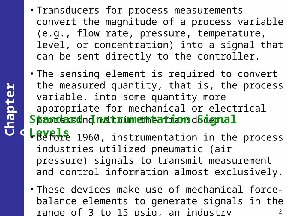
• Transducers for process measurements convert the magnitude of a process variable (e.g., flow rate, pressure, temperature, level, or concentration) into a signal that can be sent directly to the controller.

• The sensing element is required to convert the measured quantity, that is, the process variable, into some quantity more appropriate for mechanical or electrical processing within the transducer.

Standard Instrumentation Signal Levels

• Before 1960, instrumentation in the process industries utilized pneumatic (air pressure) signals to transmit measurement and control information almost exclusively.

• These devices make use of mechanical force-balance elements to generate signals in the range of 3 to 15 psig, an industry standard.

3

Ch

apte

r 9

• Since about 1960, electronic instrumentation has come into widespread use.

Sensors

The book briefly discusses commonly used sensors for the most important process variables. (See text.)

Transmitters• A transmitter usually converts the sensor output to a signal level

appropriate for input to a controller, such as 4 to 20 mA.

• Transmitters are generally designed to be direct acting.

• In addition, most commercial transmitters have an adjustable input range (or span).

• For example, a temperature transmitter might be adjusted so that the input range of a platinum resistance element (the sensor) is 50 to 150 °C.

4

Ch

apte

r 9

• In this case, the following correspondence is obtained:

Input Output

50 °C 4 mA

150 °C 20 mA

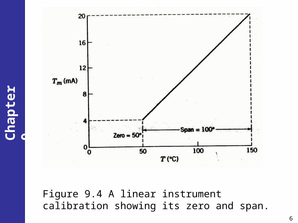
• This instrument (transducer) has a lower limit or zero of 50 °C and a range or span of 100 °C.

• For the temperature transmitter discussed above, the relation between transducer output and input is

20 mA 4 mAmA 50 C 4 mA

150 C 50 C

mA0.16 C 4 mA

C

mT T

T

5

Ch

apte

r 9

The gain of the measurement element Km is 0.16 mA/°C. For any linear instrument:

range of instrument output(9-1)

range of instrument inputmK

Final Control Elements

• Every process control loop contains a final control element (actuator), the device that enables a process variable to be manipulated.

• For most chemical and petroleum processes, the final control elements (usually control valves) adjust the flow rates of materials, and indirectly, the rates of energy transfer to and from the process.

6

Ch

apte

r 9

Figure 9.4 A linear instrument calibration showing its zero and span.

7

Ch

apte

r 9

Control Valves

• There are many different ways to manipulate the flows of material and energy into and out of a process; for example, the speed of a pump drive, screw conveyer, or blower can be adjusted.

• However, a simple and widely used method of accomplishing this result with fluids is to use a control valve, also called an automatic control valve.

• The control valve components include the valve body, trim, seat, and actuator.

Air-to-Open vs. Air-to-Close Control Valves

• Normally, the choice of A-O or A-C valve is based on safety considerations.

8

Ch

apte

r 9

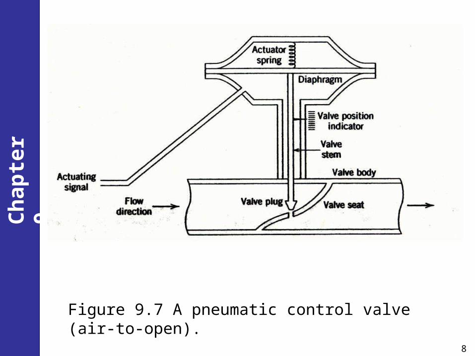
Figure 9.7 A pneumatic control valve (air-to-open).

9

Ch

apte

r 9

• We choose the way the valve should operate (full flow or no flow) in case of a transmitter failure.

• Hence, A-C and A-O valves often are referred to as fail-open and fail-closed, respectively.

Example 9.1

Pneumatic control valves are to be specified for the applications listed below. State whether an A-O or A-C valve should be used for the following manipulated variables and give reason(s).

a) Steam pressure in a reactor heating coil.

b) Flow rate of reactants into a polymerization reactor.

c) Flow of effluent from a wastewater treatment holding tank into a river.

d) Flow of cooling water to a distillation condenser.

10

Ch

apte

r 9

Valve Positioners

Pneumatic control valves can be equipped with a valve positioner, a type of mechanical or digital feedback controller that senses the actual stem position, compares it to the desired position, and adjusts the air pressure to the valve accordingly.

Specifying and Sizing Control Valves

A design equation used for sizing control valves relates valve lift to the actual flow rate q by means of the valve coefficient Cv, the proportionality factor that depends predominantly on valve size or capacity:

(9-2)vv

s

Pq C f

g

11

Ch

apte

r 9

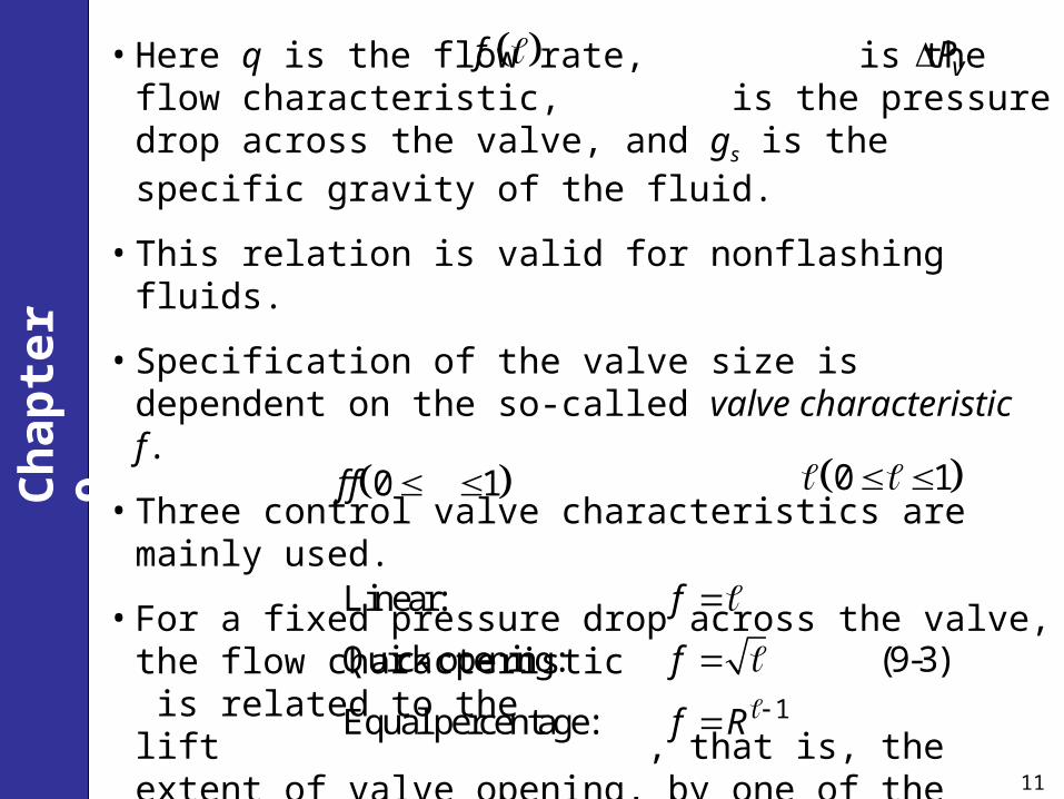
• Here q is the flow rate, is the flow characteristic, is the pressure drop across the valve, and gs is the specific gravity of the fluid.

• This relation is valid for nonflashing fluids.

• Specification of the valve size is dependent on the so-called valve characteristic f.

• Three control valve characteristics are mainly used.

• For a fixed pressure drop across the valve, the flow characteristic is related to the lift , that is, the extent of valve opening, by one of the following relations:

f vP

0 1f f 0 1

1

Linear:

Quick opening: (9-3)

Equal percentage:

f

f

f R

12

Ch

apte

r 9

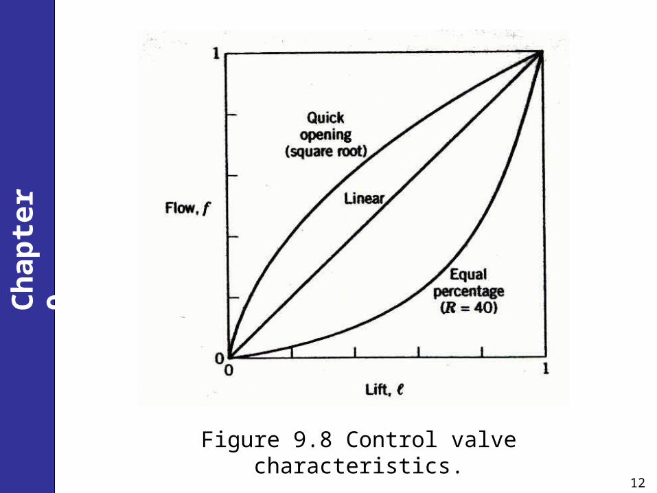
Figure 9.8 Control valve characteristics.

13

Ch

apte

r 9

where R is a valve design parameter that is usually in the range of 20 to 50.

RangeabilityThe rangeability of a control valve is defined as the ratio of maximum to minimum input signal level. For control valves, rangeability translates to the need to operate the valve within the range 0.05 ≤ f ≤ 0.95 or a rangeability of 0.95/0.05 = 19.

To Select an Equal Percentage Valve:

a) Plot the pump characteristic curve and , the system pressure drop curve without the valve, as shown in Fig. 9.10. The difference between these two curves is . The pump should be sized to obtain the desired value of , for example, 25 to 33%, at the design flow rate qd.

sP

vP/v sP P

14

Ch

apte

r 9

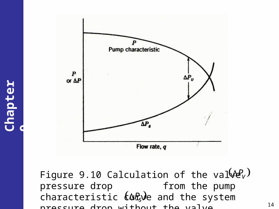
Figure 9.10 Calculation of the valve pressure drop from the pump characteristic curve and the system pressure drop without the valve

vP

.sP

15

Ch

apte

r 9

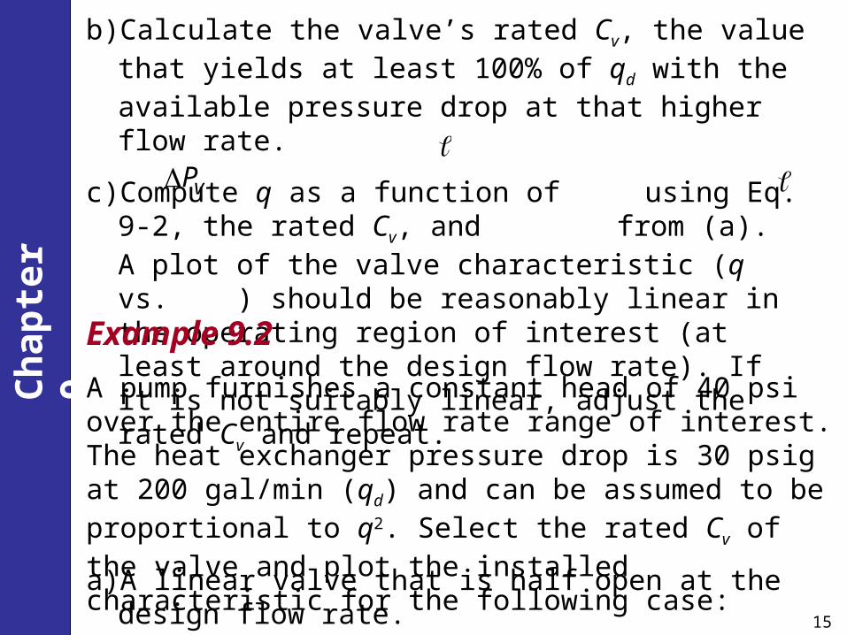
b) Calculate the valve’s rated Cv, the value that yields at least 100% of qd with the available pressure drop at that higher flow rate.

c) Compute q as a function of using Eq. 9-2, the rated Cv, and from (a). A plot of the valve characteristic (q vs. ) should be reasonably linear in the operating region of interest (at least around the design flow rate). If it is not suitably linear, adjust the rated Cv and repeat.

vP

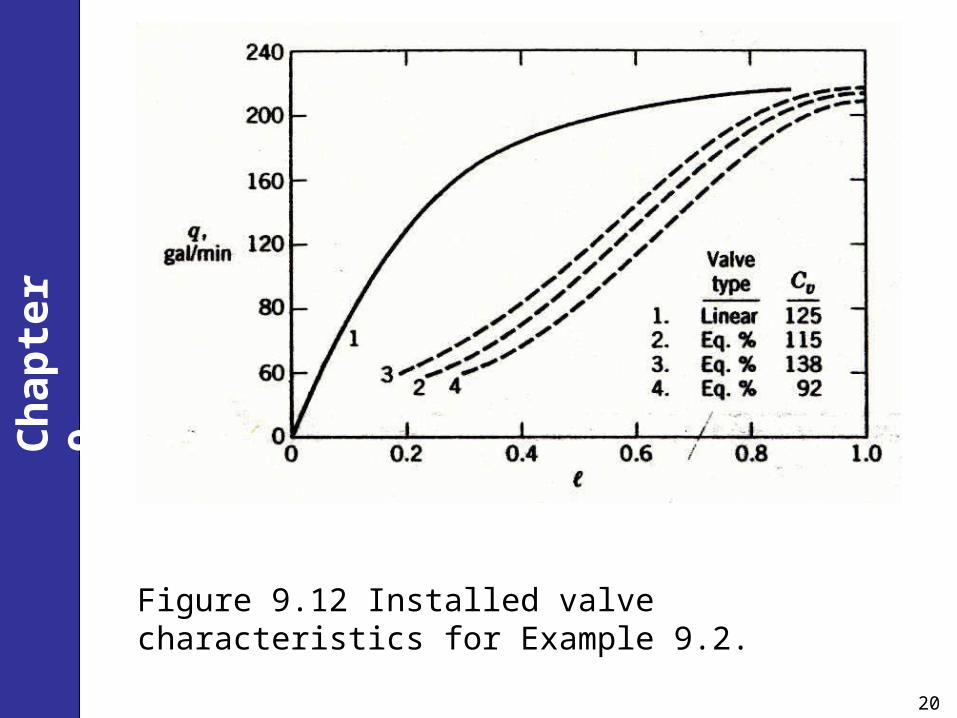
Example 9.2

A pump furnishes a constant head of 40 psi over the entire flow rate range of interest. The heat exchanger pressure drop is 30 psig at 200 gal/min (qd) and can be assumed to be proportional to q2. Select the rated Cv of the valve and plot the installed characteristic for the following case:

a) A linear valve that is half open at the design flow rate.

16

Ch

apte

r 9

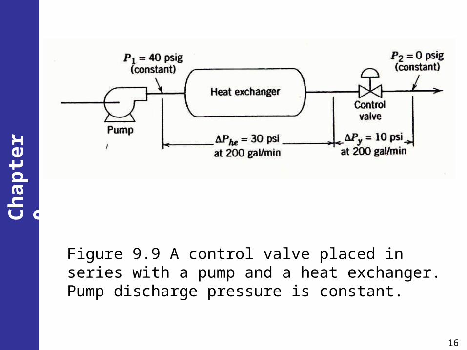
Figure 9.9 A control valve placed in series with a pump and a heat exchanger. Pump discharge pressure is constant.

17

Ch

apte

r 9

Solution

First we write an expression for the pressure drop across the heat exchanger

2

(9-5)30 200

heP q

2

30 (9-6)200s heq

P P

Because the pump head is constant at 40 psi, the pressure drop available for the valve is

2

40 40 30 (9-7)200v heq

P P

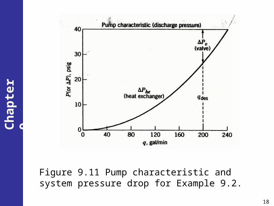
Figure 9.11 illustrates these relations. Note that in all four design cases at qd./ 10 / 30 33%v sP P

18

Ch

apte

r 9

Figure 9.11 Pump characteristic and system pressure drop for Example 9.2.

19

Ch

apte

r 9

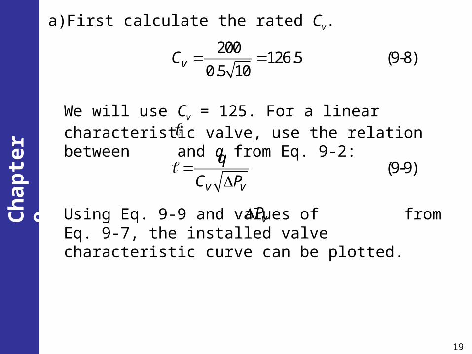
a) First calculate the rated Cv.

200126.5 (9-8)

0.5 10vC

We will use Cv = 125. For a linear characteristic valve, use the relation between and q from Eq. 9-2:

(9-9)v v

q

C P

Using Eq. 9-9 and values of from Eq. 9-7, the installed valve characteristic curve can be plotted.

vP

20

Ch

apte

r 9

Figure 9.12 Installed valve characteristics for Example 9.2.

21

Ch

apte

r 9

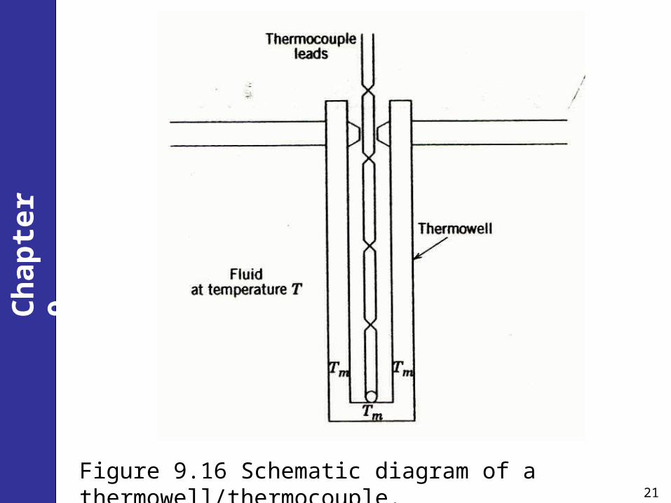
Figure 9.16 Schematic diagram of a thermowell/thermocouple.

22

Ch

apte

r 9

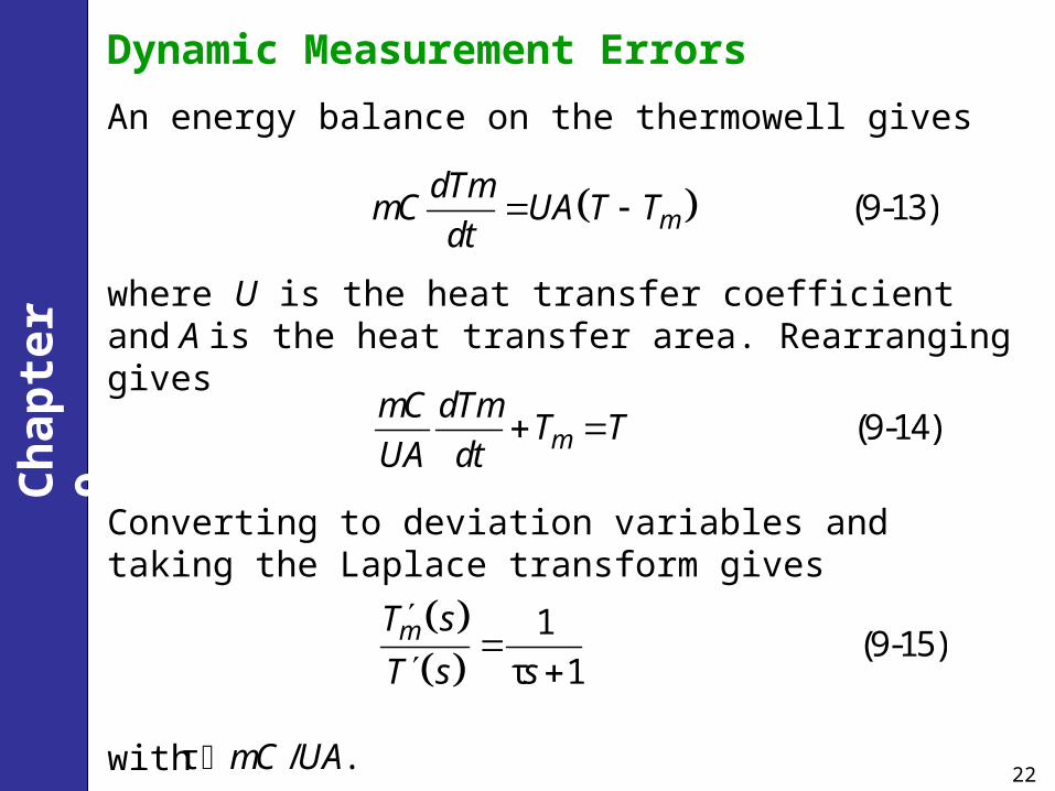
Dynamic Measurement Errors

An energy balance on the thermowell gives

(9-13)mdTm

mC UA T Tdt

where U is the heat transfer coefficient and A is the heat transfer area. Rearranging gives

(9-14)mmC dTm

T TUA dt

Converting to deviation variables and taking the Laplace transform gives

1(9-15)

τ 1mT s

T s s

with τ / .mC UA

23

Ch

apte

r 9

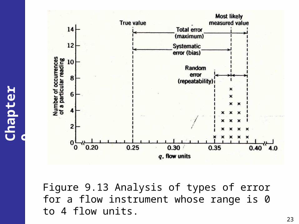
Figure 9.13 Analysis of types of error for a flow instrument whose range is 0 to 4 flow units.

24

Ch

apte

r 9

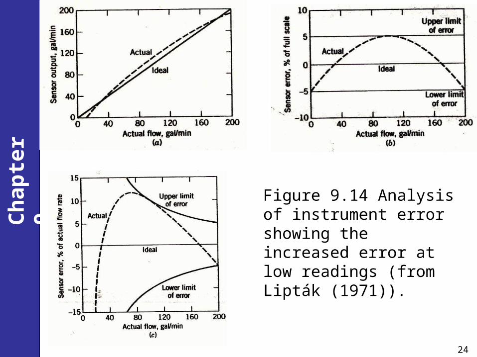
Figure 9.14 Analysis of instrument error showing the increased error at low readings (from Lipták (1971)).

25

Ch

apte

r 9

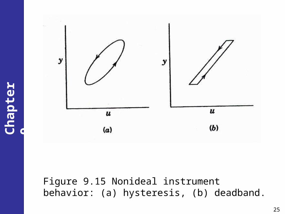
Figure 9.15 Nonideal instrument behavior: (a) hysteresis, (b) deadband.