Chapter 9 0 This document is copyrighted 2015 by Marshall ...people.emich.edu/jthomsen/Thermodynamics/ch9.pdf · Chapter 9 Copyright 2015 Marshall Thomsen 1 Modeling Real Thermodynamic

Chapter 9

Copyright 2015 Marshall Thomsen

0

This document is copyrighted 2015 by Marshall Thomsen. Permission is granted for those affiliated with academic institutions, in particular students and instructors, to make unaltered printed or electronic copies for their own personal use. All other rights are reserved by the author. In particular, this document may not be reproduced and then resold at a profit without express written permission from the author.

Problem solutions are available to instructors only. Requests from unverifiable

sources will be ignored.

Chapter 9


1

Modeling Real Thermodynamic Cycles While the Carnot cycle is useful in its simplicity, it does not adequately model

cycles commonly found in practical engines, refrigerators, or heat pumps. The focus of this chapter is modeling practical cycles. We will usually continue to assume all processes in each cycle are reversible so that these cycles will continue to be idealizations. The efficiencies we compute, then will still represent upper limits of what is achievable rather than what one may reasonably expect in actual operation. Nevertheless, by understanding these upper limits and what determines them, we can gain insight into how the efficiency of practical engines may be improved.

When Cycles Are Not Ideal Before we begin looking at new cycles, we will first briefly consider what

happens when there are irreversible processes in ideal cycles. We have seen a number of ways in which a process can be irreversible. For instance, when the state of the working fluid is changed rapidly, the fluid is forced into a non-equilibrium state. As the system evolves back into an equilibrium state, there is an entropy change associated with the irreversible nature of the process. If there is a dissipative force present, such as friction, then energy that is otherwise destined for work is instead converted to thermal energy. Associated with this increase in thermal energy is an irreversible increase in entropy.

Regardless of how the excess entropy is created, the only way to get rid of it (as

required to keep this set of processes cyclic) is to exhaust more heat. Additional heat exhaust leaves less energy available for work output, so the efficiency of a real cycle is less than that of an ideal cycle.

Example 9.1: A heat engine takes in 20 kJ of energy each cycle from a

reservoir at 500K. It exhausts heat into a reservoir at 300K. Discuss the constraints the First and Second Laws of Thermodynamics place on this engine.

The First Law of Thermodynamics gives the constraint Qexhaust +Wout = 20kJ ,

where Wout is the work done by the fluid on its surroundings. Due to friction and other losses, not all of that work will be available to accomplish the task of the engine. The Second Law of Thermodynamics places a constraint on heat flows. In order to ensure that entropy increases associated with both heat uptake and irreversible process are offset by an appropriate entropy decrease, we require

Chapter 9


2

ΔSexhaust = ΔSheat in +ΔSirrevQexhaust

TL=Qinto sys

TH+ΔSirrev

Qexhaust

300K≥20kJ500K

or, Qexhaust ≥12kJ . Finally, comparing this to the First Law constraint, we find that the

maximum work we can get out of each cycle is 8 kJ.

Work in an Open System Three of the cycles in this chapter involve fluids flowing through devices in

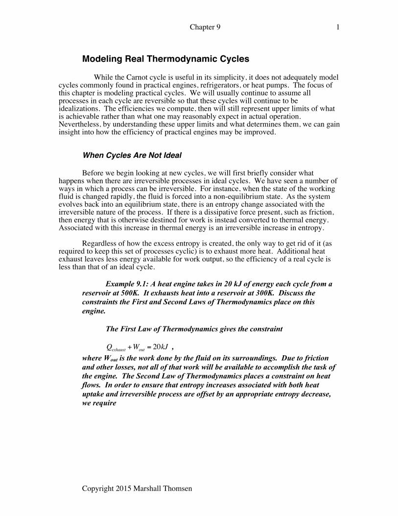
such a way that we are forced to describe the process as involving open systems, that is, systems in which mass may cross the boundary. One such process arises when a fluid, such as water vapor, flows through a turbine. A turbine is a set of blades attached to a shaft and may look like a modified fan. As fluid flows against and past the blades, the shaft is caused to rotate. This is how work may be extracted from the working fluid. The rotating shaft can be attached to an electrical generator or some other machine in order to use this work.

P1 P2 δV1 δV2

Figure 9.1 A schematic representation of a turbine. This representation can also be used for a compressor.

Chapter 9


3

Let us first imagine the following situation: a turbine, which we schematically represent by a box in Figure 9.1, has an inlet pipe and an outlet pipe, each containing a piston. By moving these two pistons, we are able to move a small amount of mass, δm, through the turbine. Defining the system as being the fluid inside the box, we see there is work δW=P1δV1 done on the system on the inlet side. The piston pushes on the fluid in the pipe, and that fluid in the pipe in turn pushes on the fluid in the box. Similarly, the work done by the system on the fluid residing in the outlet pipe is P2δV2. The net boundary work done on the system is then P1δV1- P2δV2. At the same time, if mass δm is pushed in on the inlet side, it carries with it thermal energy in the amount u1δm. The exiting thermal energy is u2δm. The total energy transmitted to the fluid inside the turbine, due to fluid flow, is

P1δV1 −P2δV2 +u1δm−u2δm = δm u1 +P1v1( )− u2 +P2v2( )"# $%= δm h1 − h2( ) . This energy can leave in the form of heat flow out of the system or work done by

the system (e.g., mechanical work done on the rotating shaft of the turbine):

δm h1 − h2( ) = δQout +δWby system . (9.1) In arriving at this equation, we have assumed no significant change in the gravitational potential energy of the fluid (i.e., no significant change in the height of the fluid) and no significant change in the kinetic energy of the fluid (i.e., no significant change in the speed of the fluid). As a first approximation for a turbine, we neglect heat loss as the fluid flows through, giving

δWby system = δm hin − hout( ) . Keeping in mind that the system is the fluid and that we are calculating the work it does on the turbine, we find δWon turbine = δm hin − hout( ) . (9.2) While work done by a fluid on a turbine results in a decrease in the enthalpy of the fluid, similar arguments show that when fluid flows through a compressor, the result is an increase in the enthalpy of that fluid: δWby compressor = δm hout − hin( ) . (9.3) An alternative expression for the work done by a compressor (or on a turbine) involves a volume-pressure integral. Consider Equation 6.25,

dH = TdS +VdP . If we assume as above that the compression is a reversible process and involves no heat flow, then it must be isentropic:

ΔH = V dP∫

Chapter 9


4

Combining this with Equation 9.3 yields

δWby compressor = δmvdP∫ . If the compressor is working on a liquid, there will be very little change in the specific volume during the process so that

δWby compressor ≈ δm Pout −Pin( )v (Liquids). (9.4) Bear in mind that the compressor is assumed to be performing work isentropically. This is in contrast to the isothermal conditions that were discussed in Chapter 5 (see Equation 5.13).

The Stirling Cycle Robert Stirling was granted a patent in 1816 on an engine designed to be more efficient than the then-popular steam engine. Over the next three decades, he and his brother James refined the design, acquired more patents, and built several working engines. The most successful was a 34 kW engine used in a foundry for almost four years. While it was apparently significantly more efficient than steam engines of the time, it broke down so frequently that it was not economically feasible to keep in operation. Improvements in materials since the Stirlings’ original patents have led to more economically feasible uses. One application is in the harnessing of solar energy (see Problem 9). A solar collector is used to concentrate radiant energy on the hot end of the Stirling engine. The work output from the engine can then be used to generate electrical energy. A second application is in the area of cooling. Refrigeration units based on the Stirling cycle turn out to be particularly effective at low temperatures (roughly 80K). The Stirling engine and the steam engine are examples of external combustion engines. Their energy source comes from outside the piston/cylinder device at the heart of the engine. This type contrasts with automobile engines that are internal combustion: the fuel is burned right in the cylinder. The Stirling cycle is an idealized model of what takes place in the Stirling engine. It consists of two constant volume (isochoric) processes alternated with two isothermal processes. There is another distinctive feature of this cycle. During the first isochoric process, heat flows out of the working fluid into a device known as a regenerator. The purpose of this device is to store thermal energy until it can be returned to the working fluid during the second isochoric process. The cycle is depicted in Figure 9.2.

Chapter 9


5

Qin

THA

THB TL

C TL

Qexhaust

THD TL

Hot side Cold side

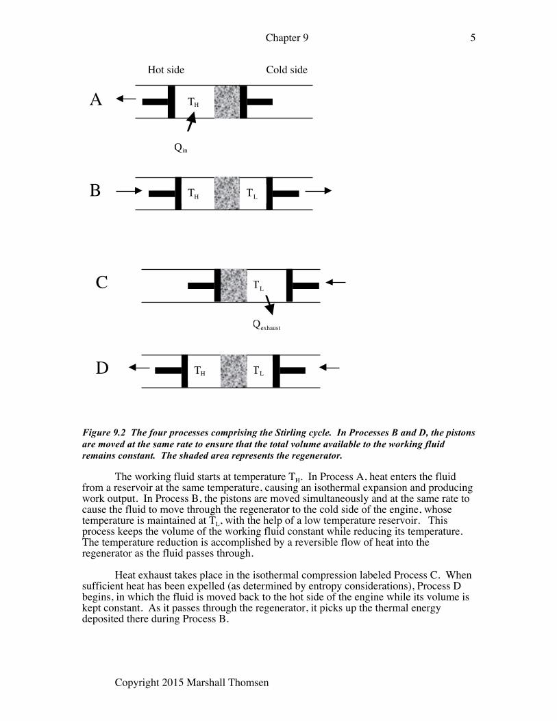
Figure 9.2 The four processes comprising the Stirling cycle. In Processes B and D, the pistons are moved at the same rate to ensure that the total volume available to the working fluid remains constant. The shaded area represents the regenerator. The working fluid starts at temperature TH. In Process A, heat enters the fluid from a reservoir at the same temperature, causing an isothermal expansion and producing work output. In Process B, the pistons are moved simultaneously and at the same rate to cause the fluid to move through the regenerator to the cold side of the engine, whose temperature is maintained at TL, with the help of a low temperature reservoir. This process keeps the volume of the working fluid constant while reducing its temperature. The temperature reduction is accomplished by a reversible flow of heat into the regenerator as the fluid passes through. Heat exhaust takes place in the isothermal compression labeled Process C. When sufficient heat has been expelled (as determined by entropy considerations), Process D begins, in which the fluid is moved back to the hot side of the engine while its volume is kept constant. As it passes through the regenerator, it picks up the thermal energy deposited there during Process B.

Chapter 9


6

The only incoming heat flow from outside the engine is found during Process A. This process is isothermal so that

Qinto sys = TH ΔS . The entropy change associated with this heat flow is what must be compensated for in the heat exhaust process (C):

Qexhaust = TL ΔS , where we have again taken advantage of the isothermal nature of the process. As we saw in Chapter 8, when the only two external heat flows involve isothermal processes, then the efficiency works out to be the same as that of the Carnot cycle. Starting from Equation 8.7,

η =1−Qexhaust

Qinto sys

=1−TL ΔSTH ΔS

=1− TLTH

(Stirling cycle). (9.5)

It is interesting to note a common feature of the Stirling and Carnot cycles.

When an ideal gas is used as a working fluid for a Stirling cycle, the heat extracted from the gas by the regenerator in Process B is identical to the heat returned by the regenerator in Process D. When an ideal gas is used as the working fluid for a Carnot cycle, the work extracted from the gas in Process B is identical to the work performed on the gas in Process D. In both cases, the same amount of energy that is pulled out of the gas in Process B is returned in Process D.

In Chapter 8, we examined a cycle similar to the Stirling cycle, called the T-V

cycle. There is a subtle but important difference between the isochoric processes in these two different cycles. In the T-V cycle, it is envisioned that the entire working fluid is always in thermal equilibrium at a single temperature at any given moment. In the first isochoric process (B), the temperature of the entire fluid is gradually and everywhere reduced from TH to TL. At any given moment, the notion of a single temperature representing the temperature of the working fluid is well defined. In the isochoric process in the Stirling cycle (also Process B), the temperature of the working fluid varies with position. The working fluid on the hot side of the engine is all at TH, that on the cold side is all at TL, and that in the regenerator varies in temperature depending on where it is in the regenerator. During this isochoric process, there is no one number we can use to represent the temperature of the entire working fluid. Since the temperature of the working fluid does not have a well-defined value for the isochoric processes, it is not possible to draw a temperature-entropy plot of the cycle as we did for the T-V cycle in Chapter 8. Likewise, it is easy to see that the pressure of the working fluid must be higher when it is on the hot side of the engine than when it is on the cold side, so there is not one value of the pressure that describes the working fluid during the isochoric processes of the Stirling cycle. For this reason, we also cannot produce a plot of pressure vs. volume for this cycle.

Returning to our general equation (9.1) for energy balance in an open system,

developed in the previous section,

δm h1 − h2( ) = δQout +δWby system

Chapter 9


7

we can calculate heat flow from the working fluid as it flows through the regenerator. The regenerator contains no moving boundary so the working fluid does no work on it. Hence

δQout = δm hincoming fluid − houtgoing fluid( ) (9.6)

That is, as the fluid moves through the regenerator in Process B, heat flows out of the working fluid as its enthalpy drops. As the fluid moves back through the regenerator in Process D, heat flows into the fluid as its enthalpy increases. In Chapter 6 we saw that the specific heat at constant pressure is closely connected to the enthalpy and hence the heat flow between the working fluid and the regenerator is governed by the specific heat at constant pressure. This is a curious result since the processes involging the regenerator take place at constant volume.

The Otto Cycle While the Stirling cycle has applications to external combustion engines,

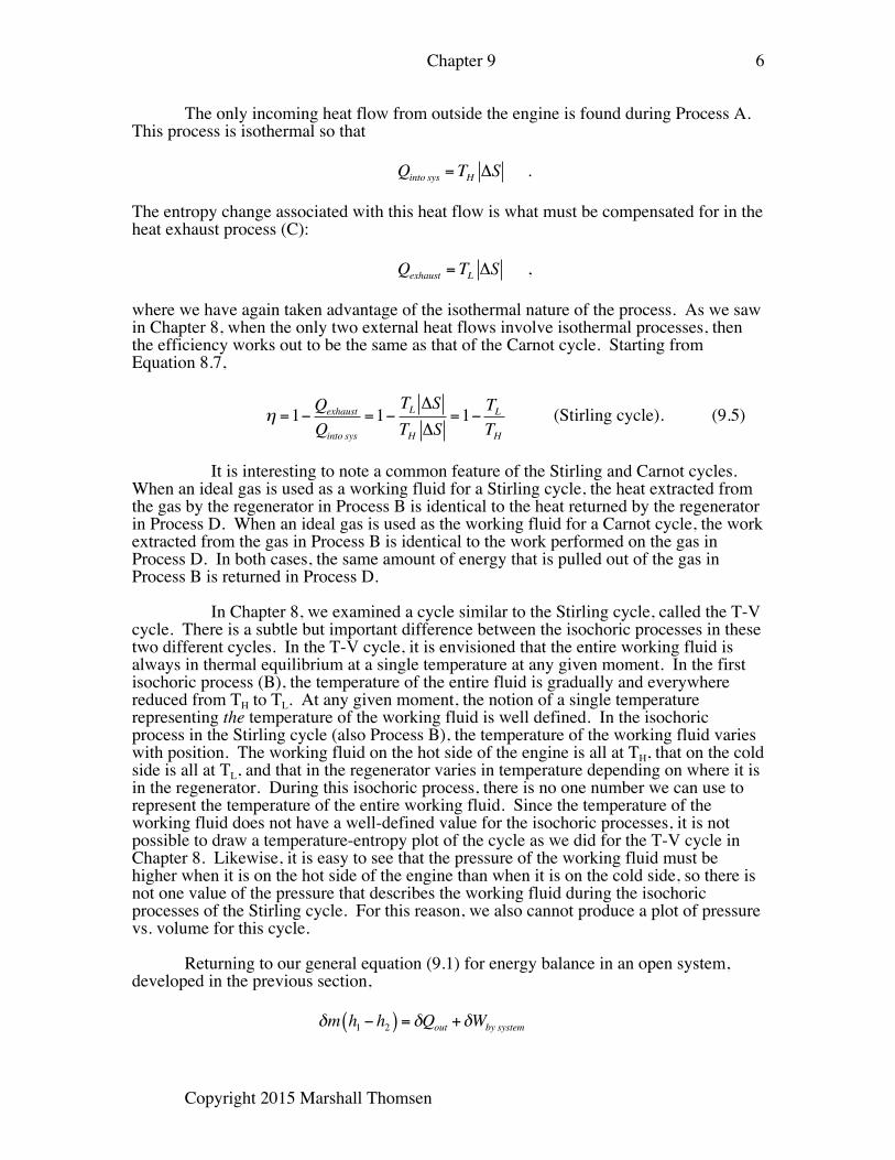
the Otto cycle models some types of internal combustion engines. We will begin with a qualitative description of a four-stroke engine cycle. From that description, we will see how the Otto cycle captures many of its essential features. The four-stroke engine begins with the intake of the air-fuel mixture as the volume of the cylinder expands. When the intake is complete, the intake valve closes, and compression of the air-fuel mixture begins. At approximately maximum compression, a spark ignites the fuel, causing rapid combustion. The combustion represents a conversion of chemical potential energy into thermal energy. The rapid rise in temperature next causes expansion in a process known as the power stroke, since it is where the output work comes from. The final process begins with the opening of the exhaust valve, allowing some gas to escape. The piston then moves back in, pushing the remaining combustion products out of the cylinder.

SparkPlug

IntakeValve

ExhaustValve

Air-FuelMixture

Figure 9.3 A schematic representation of the combustion chamber in a four-stroke engine.

Chapter 9


8

In developing an ideal cycle to model this engine, several simplifications are

made. The most significant simplification is that the working fluid is taken to be confined in a closed system. In the real four-stroke engine, the entrance of the air-fuel mixture and the exit of the combustion products are clear signs of an open system. However, many of the same features can be captured with a closed system model.

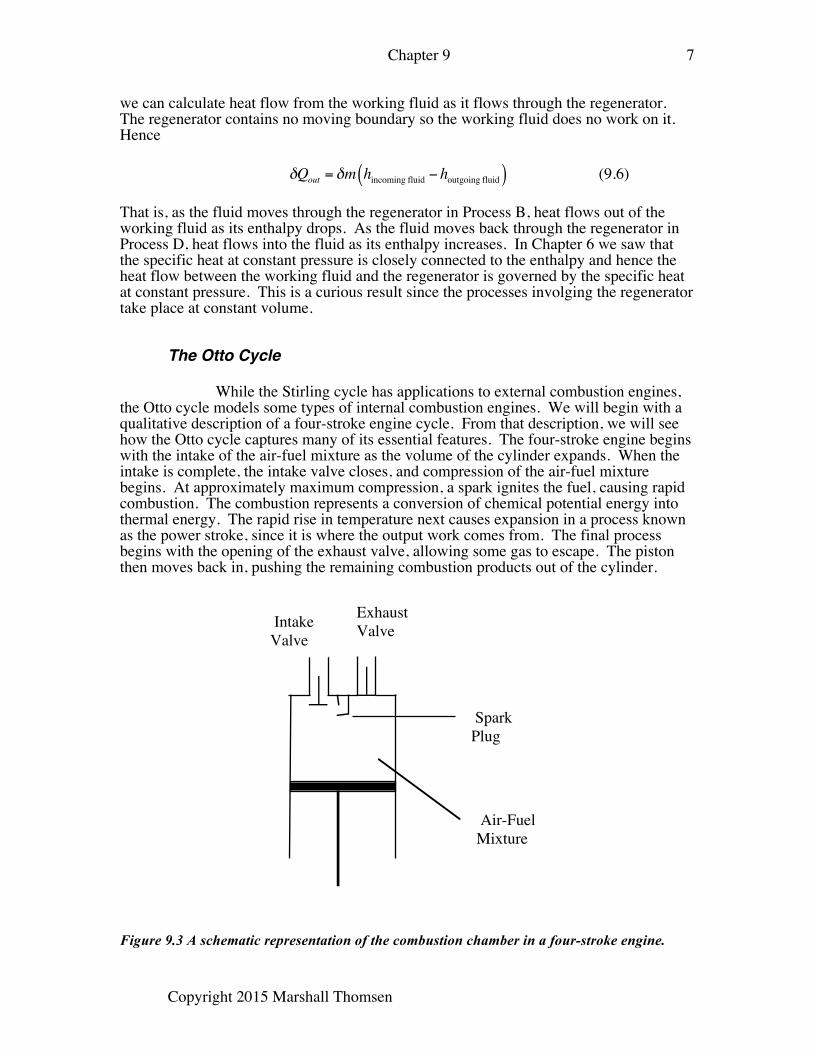
Figure 9.4 The Otto cycle is shown in the pressure-volume plane.

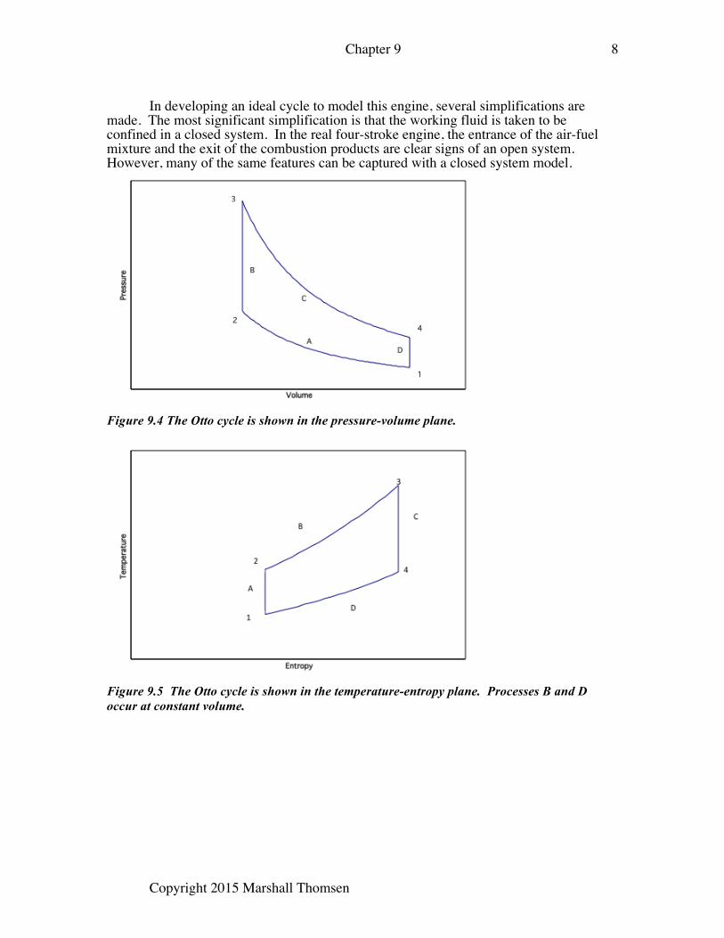
Figure 9.5 The Otto cycle is shown in the temperature-entropy plane. Processes B and D occur at constant volume.

Chapter 9


9

Process A of the idealized Otto cycle is an isentropic compression, mimicking the

air-fuel compression in the real cycle. In modeling the compression this way, we are assuming reversibility and that the compression stroke occurs rapidly enough that there is insufficient time for any significant heat flow to occur. Process B models the combustion of the fuel. In our model, we can no longer rely on the conversion in the working fluid of chemical potential energy to thermal energy as our thermal energy source. Fuel can only be burned once—there is no way to replenish it in the closed system we wish to have in our model. Thus we model this conversion in the real system by a corresponding amount of heat flow into our model closed system. Since combustion occurs rapidly, there is little chance for the volume of the working fluid to change. Therefore, in the Otto cycle we assume the heat enters in a constant volume process. Process C is the power stroke, modeled (for reasons similar to those for Process A) as an isentropic expansion. Process D is modeled as an isochoric heat exhaust to account for the thermal energy lost when exhaust gases are expelled in the real four-stroke engine.

The working fluid we will use in our model cycle is an ideal gas of constant

quantity (as measured in moles). While in the real four-stroke engine, combustion presumably changes the number of moles of gas present, the majority of the molecules in the chamber do not take part in the chemical reactions. We use the ideal gas model since at the relevant temperatures, the air in the chamber is well away from its condensation point.

We will make the further assumption that the specific heat of air is constant

during the cycle. While this approximation allows us to develop a compact expression for the efficiency of the Otto cycle, it is a bit more of a stretch. There is, in fact, a significant variation in the specific heat of air over the relevant temperature range for this cycle, a point that will be explored below in Example 9.2. Since the molecular composition of the gas changes due to combustion, we also would expect the specific heat of the gas in the chamber to be different before and after combustion even in the absence of temperature dependence. We ignore this effect too, assuming that the properties of the gas in the chamber are dominated by the air that is present.

In determining the efficiency of the cycle, it is easiest to begin from Equation 8.7:

η =1−Qexhaust

Qinto sys

Heat enters in Process B at constant volume. Since we assume cv is constant, we can write

Qinto sys =mcv T3 −T2( ) . (9.7) Likewise, in the heat exhaust process (D), we have

Qexhaust =mcv T4 −T1( ) . (9.8) Thus,

Chapter 9


10

η =1−mcv T4 −T1( )mcv T3 −T2( )

=1− T4 −T1T3 −T2

. (9.9)

While the efficiency would seem to depend on the temperatures of the four different states at the end of the four processes in the cycle, those temperatures are related to each other. In particular, since Processes A and C are isentropic ideal gas processes with constant specific heats, we can apply the result of Problem 9 in Chapter 6 to get

T1V1γ−1 = T2V2

γ−1 T3V3γ−1 = T4V4

γ−1 . We define the compression ratio as the factor by which the gas is compressed in Process A:

r = V1V2

. (9.10)

Since V1=V4 and V2=V3,

r = V4V3

.

We can then rewrite the isentropic relations as

T2T1= rγ−1 = T3

T4 . (9.11)

Now returning to Equation 9.9, we can simplify the efficiency as

η =1− T4 −T1T3 −T2

=1−T4 1−

T1T4

"

#$

%

&'

T3 1−T2T3

"

#$

%

&'

=1− T4T3

, (9.12)

where T1/T4=T2/T3 follows from Equation 9.11. Finally, we replace the temperature ratio with the compression ratio, once again using Equation 9.11:

η =1− 1rγ−1

(Otto cycle using an ideal gas with constant specific heat) (9.13)

It is thus seen that increasing the compression ratio increases the efficiency of the Otto cycle. A conventional gas powered automobile engine is spark-based. That is, it is designed to use a spark to ignite the compressed fuel. The proper timing of ignition is essential to smooth operation of the engine. However, if the air-fuel mixture is compressed too much, it can become so hot it will ignite itself, giving rise to the phenomenon known as engine knock. This phenomenon puts a practical upper limit on the compression ratio, r.

Chapter 9


11

The exact upper limit depends in part on the details of the gasoline used. Typically, automobile gasoline engines operate with a compression ratio in the range of 7 – 10.

Example 9.2: Consider an Otto cycle with air as the working fluid, for which the compression ratio is set to be 9.0, T1=300 K, and 500 kJ/kg of heat flows into the working fluid during Process B. Assume the air behaves like an ideal gas with constant specific heats. Determine the maximum temperature of the air during the cycle.

The room temperature value of cV for air is 0.718 kJ/kg K and the

room temperature value for γ (air) is 1.402 (see Appendix D). We calculate T2 using equation 9.11:

T2 = r

γ−1T1 = 9.0( )1.402−1 300K( ) = 726K T3 then follows from equation 9.7: qinto sys = cv T3 −T2( )500 kJ

kg = 0.718 kJkg K T3 − 726K( )

T3 =1422K .

This is a substantial temperature increase. In fact, for this temperature,

cV for air is about 0.92 kJ/kg K, some 28% higher than the value we assumed for our calculations. Thus there is good reason to doubt the quantitative accuracy of our result. A more careful calculation would account for the temperature dependence of the specific heat (see Problem 5).

The Rankine Cycle

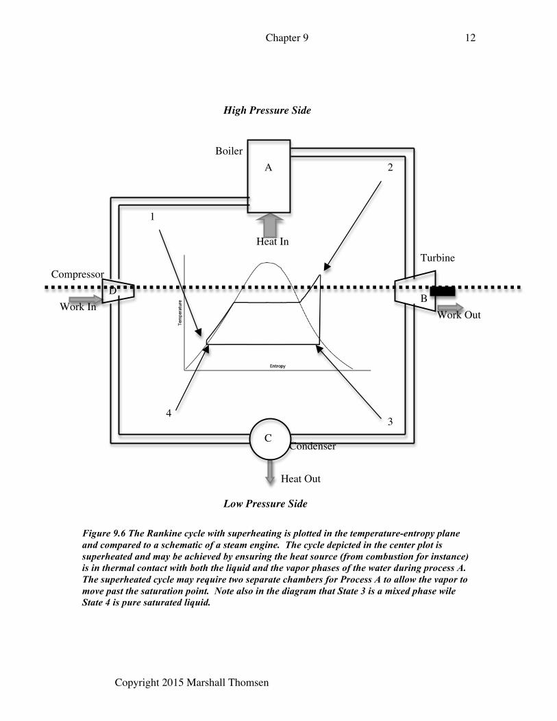
The Rankine cycle is used to model steam engines and generators. It is an idealized cycle in that each process is assumed to be reversible. The cycle is depicted in Figure 9.6. Process A involves heat entering a boiler, causing the working fluid to change from the liquid to the vapor phase. Process A often concludes with additional heat being added to the working fluid to move it out of saturation. This final portion of Process A, if present, is known as superheating. Superheating improves the efficiency of the cycle and reduces the amount of water in the liquid phase that is present in the turbine. Process A is modeled as being isobaric. The hot vapor flows into the turbine next where, in Process B, it does work on the turbine, causing the blades to turn. This process is modeled as adiabatic since it occurs too rapidly for any significant heat flow to take place. Given the additional assumption of the cycle being reversible, we can also describe Process B as isentropic. The working fluid exits the turbine as a saturated vapor/liquid. It enters the condenser where, in Process C, heat leaves the working fluid at constant pressure. The working fluid exits the condenser in the saturated liquid state. From here, the liquid flows into the compressor for Process D. This process is modeled as isentropic for the same reason Process B is. When the working fluid exits the compressor, it is ready to start the cycle over again at the boiler.

Chapter 9


12

Figure 9.6 The Rankine cycle with superheating is plotted in the temperature-entropy plane and compared to a schematic of a steam engine. The cycle depicted in the center plot is superheated and may be achieved by ensuring the heat source (from combustion for instance) is in thermal contact with both the liquid and the vapor phases of the water during process A. The superheated cycle may require two separate chambers for Process A to allow the vapor to move past the saturation point. Note also in the diagram that State 3 is a mixed phase wile State 4 is pure saturated liquid.

A Boiler

B

Turbine

C Condenser

D Compressor

High Pressure Side

Low Pressure Side

1

2

4 3

Heat In

Work Out Work In

Heat Out

Chapter 9


13

By increasing the pressure on the fluid during the compression process, we cause it to enter the coexistence region at a higher temperature than when it passes back through during the heat exhaust process (C). As can be seen in Figure 9.6, this results in a greater area enclosed in the temperature-entropy plane. Since the net work done during the cycle is equal to the area enclosed by the temperature-entropy plot, we can see why compression is useful.

When we examine the temperature-entropy plot of the cycle, we can see that most of

the heat uptake and exhaust is associated with phase changes. The large heat flow associated with a phase change allows the whole cycle to occur over a much smaller temperature range than would otherwise be possible. The price paid for this advantage is that when this cycle is run with water, the liquid phase tends to degrade engine parts more rapidly than if the entire cycle were in the vapor phase.

We now turn our attention to determining the efficiency of the cycle. Heat enters the

working fluid in Process A. Since this process is isobaric, we can write for a bit of mass δm, moving through the boiler,

δQin = δmΔh = δm h2 − h1( ) . (9.14)

The heat exhaust occurs in the condenser, and this is also an isobaric process:

δQexhaust = δmΔh = δm h3 − h4( ) , (9.15)

where as usual δQexh is defined as a positive quantity. The efficiency of the cycle is then

η =1−Qexhaust

Qin

=1− h3 − h4h2 − h1

(Rankine cycle). (9.16)

Alternatively, note that work is involved in Processes B and D, using the turbine and compressor, respectively. According to equation 9.2,

δWon turbine = δm hin − hout( ) = δm h2 − h3( ) , while the work done by the compressor on the fluid is, according to equation 9.3,

δWby compressor = δm hout − hin( ) = δm h1 − h4( ) . Thus the net work by the fluid during the cycle is

δWnet,cycle = δm h2 − h3( )−δm h1 − h4( ) = δm h2 − h1( )− h3 − h4( )"# $% . Using equation 9.14 for the input heat gives us an expression for the efficiency of the cycle identical to what we found above:

η =δWnet,cycle

δQin

=δm h2 − h1( )− h3 − h4( )"# $%

δm h2 − h1( )=1−

h3 − h4( )h2 − h1( )

.

Chapter 9


14

Example 9.3: Suppose a steam engine operates using a Rankine cycle.

The water enters the turbine at 400oC and with a pressure of 5.0 MPa. The specific enthalpy and entropy of this state are 3196.7 kJ/kg and 6.6483 kJ/kg K, respectively. The water leaves the condenser at 60 kPa. Calculate the maximum possible efficiency of this engine.

In order to calculate the efficiency, we need to determine the specific

enthalpy of each of the four states in the cycle that mark the beginning of the next process. From Figure 9.6, we see that state 2 corresponds to the water vapor just before it enters the turbine. We are given that the pressure and temperature at that point are 5.0 MPa and 400oC, respectively, and that h2=3196.7 kJ/kg and s2=6.6483 kJ/kg K.

The work done in the turbine is modeled as isentropic, so we know that

s3= s2=6.6483 kJ/kg K. Furthermore, the condensation process (C) is isobaric, so that P3=P4=60 kPa. We now have two specific pieces of information about state 3, which in principle is enough to completely define that state. By looking up the values of sliquid and sg at 60 kPa in Appendix F, we see that sliquid<s3<sg, so state 3 is a liquid/vapor coexistence state. (The notation “sliquid” for the specific entropy of saturated liquid is adopted here and elsewhere in this chapter to distinguish it more clearly from s1, the specific entropy of state 1.) We can calculate the quality, x, of the state:

s3 = 1− x( )sliquid + xsg6.6483 kJ

kg•K = 1− x( )1.1454 kJkg•K + x7.5311 kJ

kg•K ,

which gives x=0.8618. From this we obtain the specific enthalpy of state 3:

h3 = 1− x( )hliquid + xhg= 1− 0.8618( ) 359.91 kJ

kg + 0.8618( ) 2652.9 kJkg

= 2336.0 kJkg ,

where the values of the enthalpy correspond to the saturated values at 60 kPa.

When the fluid exits the condenser in state 4, it is saturated liquid at 60

kPa, so h4=359.91 kJ/kg. To obtain h1, we first use equation 9.4:

δWby compressor ≈ δm Pout −Pin( )v .

Chapter 9


15

We know that Process A is isobaric so that P2=P1=Pout=5.0 MPa. Furthermore, Pin=P4=60 kPa. Defining the work per unit mass of fluid moving through the compressor as w=δW/δm, we find

wby compressor = vliquid@60kPa P1 −P4( )

=1.03307×10−3 m3kg 5000kPa− 60kPa( )

= 5.10 kJkg .

Finally, from equation 9.3,

δWby compressor = δm hout − hin( )wby compressor = h1 − h4h1 = wby compressor + h4 = 359.91 kJ

kg + 5.10 = 365.01 kJkg .

Having completed our task of determining the specific enthalpies, we

can now calculate the efficiency from equation 9.16:

η =1− h3 − h4h2 − h1

=1−2336.0 kJ

kg −359.91 kJkg

3196.7 kJkg −365.01 kJ

kg

= 0.302 .

Since this is the efficiency for an ideal Rankine cycle, it represents the

upper limit of the actual efficiency of a steam engine operating under these conditions. Real efficiencies can be substantially lower due to dissipation and other irreversibilities.

Vapor Compression Refrigeration Cycle We now turn our attention to a cycle used in refrigeration processes. We begin by

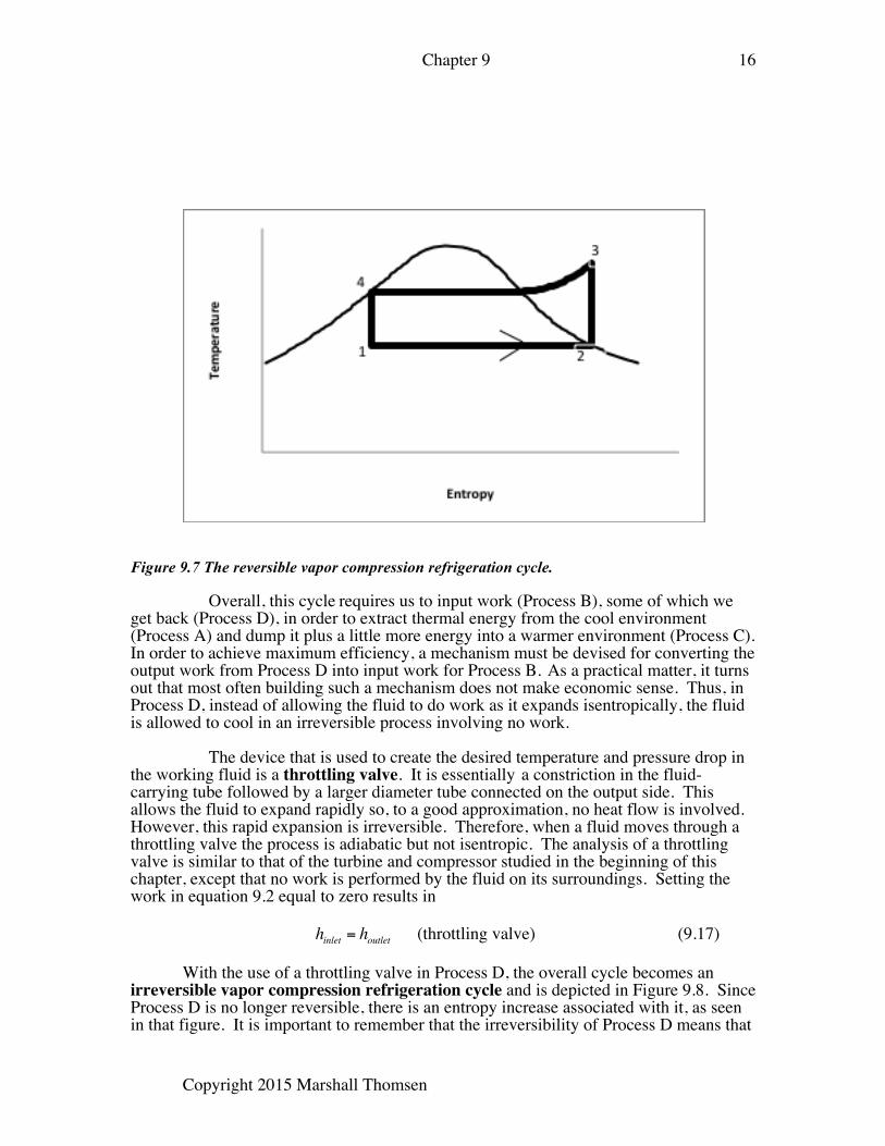
modeling a reversible refrigeration cycle, as depicted in Figure 9.7. In state 1, the working fluid is in liquid-vapor coexistence. During Process A, heat enters the fluid under isobaric conditions, until all of the liquid has become vapor. This is the essential function of the cycle, to absorb thermal energy from a room or from a refrigerated compartment. The remaining processes are present to dump this thermal energy elsewhere and complete the cycle. Process B is an isentropic compression that raises the temperature of the vapor. Now that the vapor is hot, heat readily flows out into the surroundings in Process C, which is taken to be isobaric. This process continues until all of the vapor has condensed to the saturated liquid state. In Process D, the fluid does work through an isentropic expansion. This causes the temperature to drop as the fluid enters liquid-vapor coexistence, returning to its starting state.

Chapter 9


16

Figure 9.7 The reversible vapor compression refrigeration cycle. Overall, this cycle requires us to input work (Process B), some of which we

get back (Process D), in order to extract thermal energy from the cool environment (Process A) and dump it plus a little more energy into a warmer environment (Process C). In order to achieve maximum efficiency, a mechanism must be devised for converting the output work from Process D into input work for Process B. As a practical matter, it turns out that most often building such a mechanism does not make economic sense. Thus, in Process D, instead of allowing the fluid to do work as it expands isentropically, the fluid is allowed to cool in an irreversible process involving no work.

The device that is used to create the desired temperature and pressure drop in

the working fluid is a throttling valve. It is essentially a constriction in the fluid-carrying tube followed by a larger diameter tube connected on the output side. This allows the fluid to expand rapidly so, to a good approximation, no heat flow is involved. However, this rapid expansion is irreversible. Therefore, when a fluid moves through a throttling valve the process is adiabatic but not isentropic. The analysis of a throttling valve is similar to that of the turbine and compressor studied in the beginning of this chapter, except that no work is performed by the fluid on its surroundings. Setting the work in equation 9.2 equal to zero results in

hinlet = houtlet (throttling valve) (9.17)

With the use of a throttling valve in Process D, the overall cycle becomes an

irreversible vapor compression refrigeration cycle and is depicted in Figure 9.8. Since Process D is no longer reversible, there is an entropy increase associated with it, as seen in that figure. It is important to remember that the irreversibility of Process D means that

Chapter 9


17

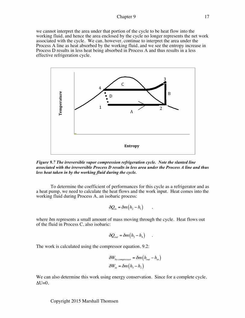
we cannot interpret the area under that portion of the cycle to be heat flow into the working fluid, and hence the area enclosed by the cycle no longer represents the net work associated with the cycle. We can, however, continue to interpret the area under the Process A line as heat absorbed by the working fluid, and we see the entropy increase in Process D results in less heat being absorbed in Process A and thus results in a less effective refrigeration cycle.

Figure 9.7 The irreversible vapor compression refrigeration cycle. Note the slanted line associated with the irreversible Process D results in less area under the Process A line and thus less heat taken in by the working fluid during the cycle.

To determine the coefficient of performances for this cycle as a refrigerator and as

a heat pump, we need to calculate the heat flows and the work input. Heat comes into the working fluid during Process A, an isobaric process:

δQin = δm h2 − h1( ) ,

where δm represents a small amount of mass moving through the cycle. Heat flows out of the fluid in Process C, also isobaric:

δQout = δm h3 − h4( ) .

The work is calculated using the compressor equation, 9.2:

δWby compressor = δm hout − hin( )δWin = δm h3 − h2( )

We can also determine this work using energy conservation. Since for a complete cycle, ΔU=0,

Chapter 9


18

Wnet, in,cycle +Qnet, in,cycle = 0

Win +δm h2 − h1( )−δm h3 − h4( ) = 0Win = δm h3 − h2( ) ,

where in the last step we have used h1=h4 due to the throttling process.

We can now obtain the coefficients of performance for the refrigeration and heat

pump cycles:

COPref =Qin

Win

=h2 − h1h3 − h2

(9.18)

and

COPHP =Qexhaust

Win

=h3 − h4h3 − h2

. (9.19)

Determining these coefficients of performance will require a detailed knowledge of the states of the working fluid, as was the case for the Rankine cycle.

Chapter 9


19

Chapter 9 Problems 1. An engine based on the Stirling cycle uses 2.2 kg of N2 as its working fluid. 570 kJ

of heat enters at a temperature of 850K during each cycle. Heat is exhausted at 330 K. You may neglect the temperature dependence of the specific heats. a. What is the ideal efficiency of the cycle? b. What is the maximum amount of work that can be obtained per cycle? c. What is the minimum amount of heat that must be exhausted during each cycle? d. How much heat is transferred to and from the regenerator during each cycle?

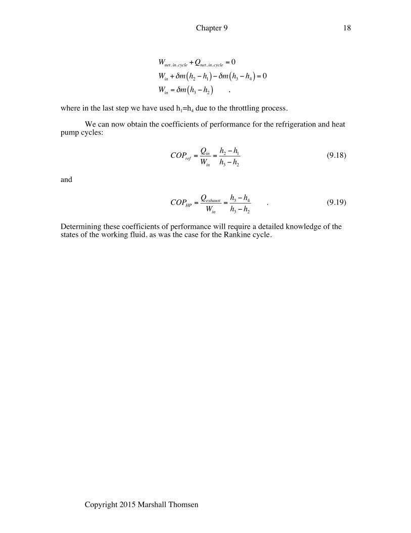
2. A plot of a Rankine cycle is shown below in the pressure vs. specific enthalpy plane.

The dashed line is the liquid-vapor coexistence curve for water. Determine the efficiency of this cycle.

Figure 9.7 The Rankine cycle described in Problem 2.

0

500

1000

1500

2000

2500

3000

3500

4000

4500

5000

0 500 1000 1500 2000 2500 3000 3500Specific Enthalpy (kJ/kg)

Pres

sure

(kP

a)

Chapter 9


20

3. In a non-superheated Rankine cycle, water leaves the boiler at saturation. Suppose such a cycle takes place with saturated water vapor entering the turbine at 3500 kPa and water (in an unknown phase) leaving the turbine at 100 kPa. Determine the efficiency of this cycle.

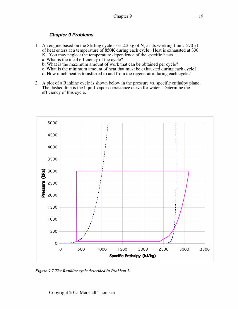
4. An irreversible vapor compression refrigeration cycle involving R-134a is shown on

the plot below. Portions of the liquid-vapor coexistence curve are shown in dashed lines for reference. a. Calculate COPR for this cycle. b. If this cycle were used in a heat pump, what would COPHP be?

Figure 9.8 The irreversible vapor compression refrigeration cycle described in Problem 4.

0

500

1000

1500

2000

2500

3000

3500

0 50 100 150 200 250 300Specific Enthalpy (kJ/kg)

Chapter 9


21

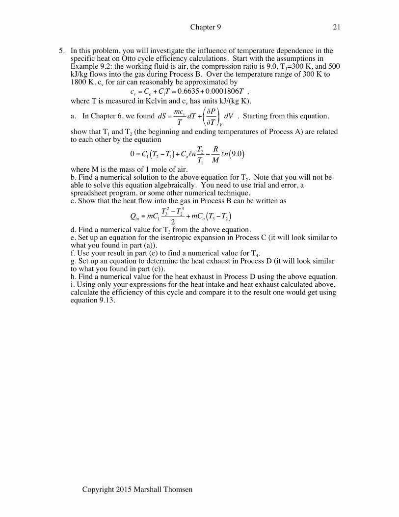
5. In this problem, you will investigate the influence of temperature dependence in the specific heat on Otto cycle efficiency calculations. Start with the assumptions in Example 9.2: the working fluid is air, the compression ratio is 9.0, T1=300 K, and 500 kJ/kg flows into the gas during Process B. Over the temperature range of 300 K to 1800 K, cv for air can reasonably be approximated by

cv =Co +C1T = 0.6635+ 0.0001806T , where T is measured in Kelvin and cv has units kJ/(kg K).

a. In Chapter 6, we found dS = mcvT

dT + ∂P∂T"

#$

%

&'V

dV . Starting from this equation,

show that T1 and T2 (the beginning and ending temperatures of Process A) are related to each other by the equation

0 =C1 T2 −T1( )+ConT2T1−RMn 9.0( )

where M is the mass of 1 mole of air. b. Find a numerical solution to the above equation for T2. Note that you will not be able to solve this equation algebraically. You need to use trial and error, a spreadsheet program, or some other numerical technique. c. Show that the heat flow into the gas in Process B can be written as

Qin =mC1T32 −T2

3

2+mCo T3 −T2( )

d. Find a numerical value for T3 from the above equation. e. Set up an equation for the isentropic expansion in Process C (it will look similar to what you found in part (a)). f. Use your result in part (e) to find a numerical value for T4. g. Set up an equation to determine the heat exhaust in Process D (it will look similar to what you found in part (c)). h. Find a numerical value for the heat exhaust in Process D using the above equation. i. Using only your expressions for the heat intake and heat exhaust calculated above, calculate the efficiency of this cycle and compare it to the result one would get using equation 9.13.

Chapter 9


22

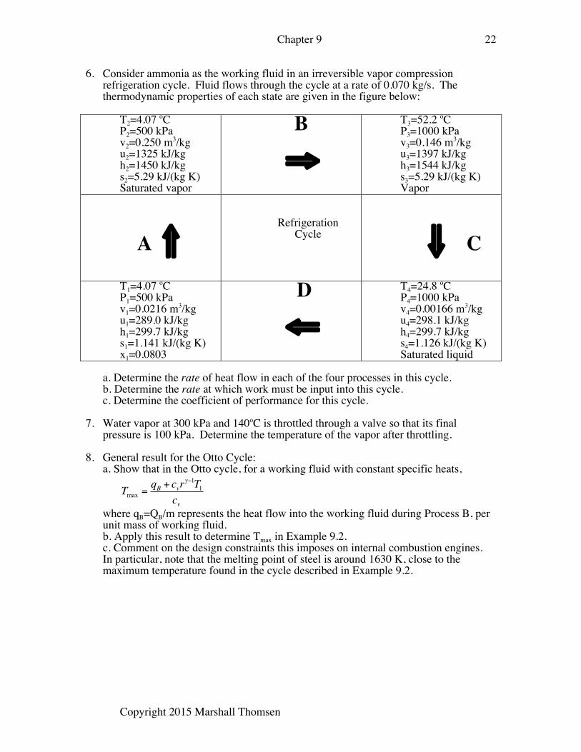
6. Consider ammonia as the working fluid in an irreversible vapor compression refrigeration cycle. Fluid flows through the cycle at a rate of 0.070 kg/s. The thermodynamic properties of each state are given in the figure below:

T2=4.07 oC P2=500 kPa v2=0.250 m3/kg u2=1325 kJ/kg h2=1450 kJ/kg s2=5.29 kJ/(kg K) Saturated vapor

B

⇒ T3=52.2 oC P3=1000 kPa v3=0.146 m3/kg u3=1397 kJ/kg h3=1544 kJ/kg s3=5.29 kJ/(kg K) Vapor

A ⇑

Refrigeration Cycle

⇓ C

T1=4.07 oC P1=500 kPa v1=0.0216 m3/kg u1=289.0 kJ/kg h1=299.7 kJ/kg s1=1.141 kJ/(kg K) x1=0.0803

D

⇐ T4=24.8 oC P4=1000 kPa v4=0.00166 m3/kg u4=298.1 kJ/kg h4=299.7 kJ/kg s4=1.126 kJ/(kg K) Saturated liquid

a. Determine the rate of heat flow in each of the four processes in this cycle. b. Determine the rate at which work must be input into this cycle. c. Determine the coefficient of performance for this cycle.

7. Water vapor at 300 kPa and 140oC is throttled through a valve so that its final

pressure is 100 kPa. Determine the temperature of the vapor after throttling. 8. General result for the Otto Cycle: a. Show that in the Otto cycle, for a working fluid with constant specific heats,

Tmax =qB + cvr

γ−1T1cv

where qB=QB/m represents the heat flow into the working fluid during Process B, per unit mass of working fluid. b. Apply this result to determine Tmax in Example 9.2. c. Comment on the design constraints this imposes on internal combustion engines. In particular, note that the melting point of steel is around 1630 K, close to the maximum temperature found in the cycle described in Example 9.2.

Chapter 9


23

9. The Solar Power and Sun Lab at Sandia National Laboratory uses a concave mirror to concentrate solar energy on a Stirling engine. The mechanical output of the Stirling engine is used to operate an electrical generator. A report indicates that solar energy is available at that site at the rate of 2.7MWh/m2/yr. Of this energy, approximately 90% is reflected by the mirror onto a receiver. In turn, approximately 90% of this energy makes it to the hot side of the Stirling engine. The high performance Stirling engine can operate at an upper temperature of 700oC.

a. Assuming the cold side of the Stirling engine is at 30oC, calculate the upper limit on the efficiency of the engine itself.

b. Combine the efficiency in part (a) with other given information to estimate an upper limit for the overall conversion efficiency of solar energy into mechanical energy by the system.

c. The report states that the overall solar-electric conversion efficiency is 29.4%. What factors might account for the discrepancy between this number and what was calculated in (b)?

d. Using the 29.4% efficiency as a guide, how large a solar collector would be required to produce an average electrical power output of 1.0 kW?

10. Show that when an ideal gas flows through a throttling valve, the inlet temperature is

equal to the outlet temperature. Make it clear at what stage(s) you need to rely on the properties of an ideal gas. (This result does not apply to non-ideal gases.)

11. Show that the heat flow into the working fluid during an irreversible vapor

compression refrigeration cycle is given by δm 1− x1( ) hg P1( )− hl P1( )"# $%

where x1 and P1 are the quality and pressure, respectively, measured in state 1. 12. The specific enthalpy of R134a for saturated vapor is reasonably well fit to the

function hg =17.9•n 0.056P + 0.0029( )+317.51

where P is in MPa and h is in kJ/kg. This gives less than 1% error over the range from 0.06 MPa to 0.80 MPa. The specific enthalpy of R134a for saturated liquid can be reasonably well fit to

hl = 81.9+35.4P −1

0.00939+ 0.0501P

where again P is in MPa and h is in kJ/kg. This gives less than 4% error over the same pressure range. Let qin denote the heat flow per unit mass into R134a during an irreversible vapor compression refrigeration cycle. a. With the help of Problem 11, show that over the pressure range of 0.06 MPa to 0.80 MP{a, qin has its maximum at 0.06 MPa and its minimum at 0.80 MPa. You may do so either by generating and submitting a plot or by showing the first derivative is negative over the entire interval. b. Taking x1=0.30, determine the maximum and minimum values for qin.

13. Suppose in Example 9.3 that the water leaves the condenser at a pressure of 100 kPa. What is the new efficiency of the cycle?

Chapter 9


24

14. Gasoline contains predominantly octane (the “octane” value quoted on the pump is approximately equal to the percent of octane in the gasoline). Octane has an auto-ignition temperature of 417oC. In the isentropic compression portion of the Otto cycle, the point is to get the air-fuel mixture hot without exceeding the auto-ignition temperature for the fuel. Estimate the upper limit on the compression ratio in this cycle such that the auto-ignition temperature is not exceeded in state 2 (just prior to spark ignition). You may assume the air-fuel mixture is an ideal gas that has a γ value of 1.4 (constant) and a temperature of 25oC.

15. Consider a Rankine cycle in which steam enters the turbine at 300oC and 1.00 MPa,

and the condenser operates at a pressure of 100 kPa. Calculate the efficiency of this cycle, assuming it is reversible. Note that these numbers are not necessarily realistic but were chosen so that data would be readily available in the appendices.

16. Suppose water is used as a working fluid in an irreversible vapor compression

refrigeration cycle. The temperature at which heat uptake occurs is 1oC and the pressure of the fluid during heat exhaust is 4.50 kPa. a. Calculate the coefficient of refrigeration performance for this cycle. You will need to use Excel files WaterGasPhase and WaterSaturation. b. Aside from the lower bound on the temperature of the heat uptake portion of the cycle being the triple point for water, can you identify other serious design concers with this refrigeration device?

17. In a Brayton cycle, Process A is an isentropic compression of the working fluid. In Process B, heat enters the fluid under isobaric conditions. In Process C, the fluid expands isentropically until the pressure is reduced to its starting value. Finally in Process D, heat is exhausted isobarically until the volume has returned to its original value. All four processes are assumed to be reversible. This cycle is an idealization of the cycle used in the Pebble Bed Nuclear Reactors (a reactor in development but not commercially viable at this point). a. Sketch the cycle in the PV plane, using conventional labeling (i.e., the cycle starts in state 1, Process A connects state 1 to state 2, etc.). b. Some references indicate the efficiency of this cycle may be expressed as

η =1− T1T2

.

Derive this equation, explaining any additional assumptions you need to make to obtain it. Do not assume this is a Carnot cycle!

c. Repeat (b) for the alternate form, η =1− P1P2

"

#$

%

&'

γ−1( )γ

Chapter 9


25

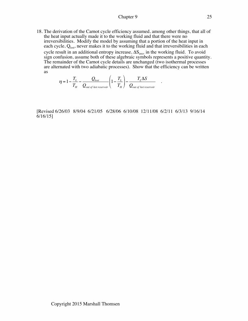
18. The derivation of the Carnot cycle efficiency assumed, among other things, that all of the heat input actually made it to the working fluid and that there were no irreversibilities. Modify the model by assuming that a portion of the heat input in each cycle, Qlost, never makes it to the working fluid and that irreversibilities in each cycle result in an additional entropy increase, ΔSirrev in the working fluid. To avoid sign confusion, assume both of these algebraic symbols represents a positive quantity. The remainder of the Carnot cycle details are unchanged (two isothermal processes are alternated with two adiabatic processes). Show that the efficiency can be written as

η =1− TLTH

−Qlost

Qout of hot reservoir

1− TLTH

"

#$

%

&'−

TLΔSQout of hot reservoir

.

[Revised 6/26/03 8/9/04 6/21/05 6/28/06 6/10/08 12/11/08 6/2/11 6/3/13 9/16/14 6/16/15]

Documents

Chapter 9 0 This document is copyrighted 2015 by Marshall ...people.emich.edu/jthomsen/Thermodynamics/ch9.pdf · Chapter 9 Copyright 2015 Marshall Thomsen 1 Modeling Real Thermodynamic