Embed Size (px)
Citation preview

Chapter 8. Some Statistical Methods for the
Design of Experiments and Analysis of
Samples
ELLIE E. PREPAS
1 Introduction
Statistical analysis can be a very powerful tool for the researcher, but its power
comes mainly from interpreting data which were collected for a specific
analysis. This chapter introduces the reader to some of the analyses used
routinely by researchers and to aspects of sampling design which should be
considered prior to the collection of field or laboratory data. It is not intended
as a substitute for a text in applied statistics (e.g., Zar 1974, Snedecor &
Cochran 1980, and Sokal & Rohlf 1981); rather it directs the reader to specific
tests and problems which are common in aquatic invertebrate research.
This chapter is divided into five parts. The introduction deals with
commonly used sample statistics and distributions. The second section
focuses on design of the experiment and the sampling program. Preparation
of data for analysis, including enumeration, volume weighting, smoothing,
determining the distribution, and transformation are introduced in the third
part. Section four deals mainly with the comparison of means, such as the t-
test, nonparametric alternatives, multiple comparisons between means, and
problems to be aware of when doing an analysis of variance. This section also
looks at tests for homogeneity of sample variances and combining
probabilities from independent tests of significance. Finally, standard
regression and correlation, and alternative methods are discussed in terms of
searching for patterns, estimating parameters and making predictions.
Many of the statistical models discussed will be illustrated with examples
from the literature, although the analyses may differ from those undertaken
by the original authors.
/./ Descriptive statistics
There are two basic kinds of sample statistics: indices of central tendency and
dispersion.
1.1.1 Indices of central tendency
The most frequently used measure of central tendency is the arithmetic mean.
266

Design of Experiments and Analysis of Samples 267
The arithmetic mean X is the average of a set of;? observations X,:
The statistic X is an estimate of the parameter f.u the true population mean.
(Greek letters such as \i are used in statistics to describe actual as opposed to
estimates of population parameters.) The mean is the measure of central
tendency used in most statistical analyses. It is thus the most powerful index of
central tendency.
The median, the value with an equal number of observations on either side
of it, is another measure of central tendency used in biological studies. It is a
useful statistic for describing a population with a skewed distribution because,
unlike the mean, it is not unduly influenced by outliers. Other indices such as
the geometric mean, harmonic mean, and mode, are rarely used in analyses of
biological data.
1.1.2 Indices of dispersion
The most commonly used indices of dispersion are the variance (s2) and the
standard deviation (.v). The variance is calculated from the sum of the squared
deviations of each observation from the mean (i.e., sum of squares), corrected
for sample size. The mean sum of squares tends to underestimate the true
population variance a2 and thus it is divided by n - I rather than /;:
(8.2)n- 1
In practice the formula used to calculate the variance is:
The standard deviation is the square root of the variance. Variance and
standard deviation are the most powerful measures of dispersion because
they, like the mean, are used for statistical analyses.
The range (i.e., the distance between the maximum and minimum values) is
also used to describe sample variation. The range is affected by outlying values
and sample size and thus is only a rough estimate of dispersion.

268 Chapter 8
1.1.3 The coefficient of variation
The coefficient of variation, CV, is a relative measure ofdispersion in a sample.
It is the ratio of the standard deviation, s, to the mean:
CV=t (8.3)
A large CV indicates substantial variation in the samples, whereas, a small CV
(i.e., 0-20 or less) indicates that the X is representative of the true population
mean n and, in samples where the s2 is not dependent on the A\ that the s2 is
representative of the true population variance a2. The CV is often used to
compare the variability of data sets measured in different units (e.g., feet as
opposed to centimeters).
The calculation ofdescriptive statistics is illustrated in Table 8.1 using data
from Ricker (1938) on the number ofDaphnia in replicate samples collected at
one location and at random locations in Cultus Lake.
7.2 Distribution of the data
Most statistical analyses assume that random processes are responsible for the
variation observed in a population. This variation may be described by
different models depending on whether the variable is discontinuous or
continuous. The binomial and related distributions are used to describe
certain discontinuous or discrete data, such as number of organisms per
sample with a particular attribute, whereas the normal distribution is used for
continuous variables, such as weight, and can also be used for most discrete
variables.
The binomial distribution is based on the parameters/?, the proportion of
the population containing a particular attribute, and q. which is denned as
1 =p. The events acting on the population are assumed to be independently
distributed and p is assumed to be constant. For a sample of size /?, \x = np and
a2 = npq. Suppose 100 copepods are taken from each of several random
samples collected from a lake. Suppose also that there is an equal sex ratio in
the population and that male copepods are randomly distributed. Then the
number ofmale copepods per sample should follow the binomial distribution,
with p = 0-5 and n = 100.
As the sample size increases, the binomial distribution tends quickly to the
normal distribution, particularly when p is close to 0-5. The normal
approximation is usually considered adequate if the mean of the population
(H =np) is greater than 15. Where p is small and fi=np< 15 the Poisson
distribution, which has the useful property /< = a2, is used. If the individuals
in a rare population are randomly distributed in a lake then the number of

Table 8.1 Calculation of sample statistics for the number of Daplmia collected in
Cultus Lake, British Columbia, from one central location and at several randomly
selected open water locations (data are from Ricker 1938).
Haul numberLocation
Centre Random
1
2
3
4
5
6
7
8
9
10
total f£ x\
sample size, n
mean X
median
variance, s'
range
standard deviation, s
cvlis2!X
37
48
37
46
38
38
50
33
35
50
412
10
33, 35, 37, 37
38, 38 = 38
46, 48, 50, 50
(412)2
= 42-8
33-50
6
6-54
41-2
1
2
■54
_r— v
•04
•07
63
54
91
83
104
79
71
545
7
54, 63,
79
83,91,
71,
= 79
104
44153-
= 286-8
54-104
16-9
169
77-9= 0-22
3-68
640
270 Chapter 8
these individuals collected in random samples should follow the Poisson
distribution. The Poisson distribution is also used to describe counts of
organisms from replicate samples.
A simple way to determine whether counts are randomly distributed is to
examine the s2 to X ratio. This ratio is close to 1 if the distribution is random
and > 1 if it is clumped or contagious. The data on Daplmia collected at one
station (Table 8.1) appear to follow the Poisson distribution because the .v2 to
X ratio is very close to unity. On the other hand, samples collected at
randomly selected stations have a s2 to X ratio which is substantially > 1,
suggesting a contagious distribution. A /2-tesl can be used to determine
whether the .v2 to X ratio is significantly different from unity (see Section 3.5).
The normal distribution has a symmetrical bell-shaped curve about the
population mean n. The breadth of the curve is determined by the variance
(<r2). The normal distribution works well for measurements such as length or
weight when the population is not skewed towards large or small individuals,
although many measurements made in biology do not conform to the normal
distribution. However, as the sample size increases, the sample means
approach normality even when the raw data are not normally distributed. In
addition, it may be possible to transform the data to a normal distribution (see
Sections 3.4-3.6). Methods of calculating the binomial, Poisson, and normal
distributions are covered in most statistical texts. Other methods for analyzing
patterns ofdiscrete variables are discussed in detail in the ecological literature
(e.g., Lloyd 1967; Pielou 1977; Elliott 1977; Iwao 1977; Green 1979).
2 Sampling Design
Preliminary data on the distribution or the characteristics of the organisms
under study can be used to estimate the number of samples required for a given
level of accuracy, to determine the best method of sampling, e.g., random,
systematic, or stratified, and where appropriate, the time interval between
samples.
2.1 Random sampling
To locate random stations for sampling, a random number table is usually
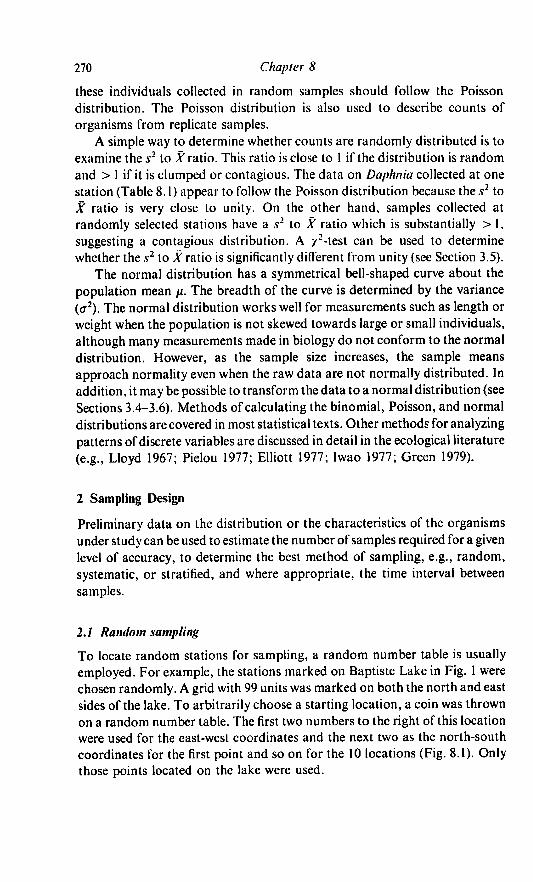
employed. For example, the stations marked on Baptiste Lake in Fig. 1 were
chosen randomly. A grid with 99 units was marked on both the north and east
sides of the lake. To arbitrarily choose a starting location, a coin was thrown
on a random number table. The first two numbers to the right of this location
were used for the east-west coordinates and the next two as the north-south
coordinates for the first point and so on for the 10 locations (Fig. 8.1). Only
those points located on the lake were used.

Design of Experiments and Analysis of Samples 271
100
90
80
70
60
50
40
30
20
10
South Basin
Baptiste Lake
40 50 60 70 80 90 100
Grid Units
54 17 67 65 56 59 44 10 54 73 61 34 83 38 66 79
23 93 05 32 49 27 08 33 43 57 88 04 05 33 64 71
Fig. 8.1 Randomly chosen sampling locations marked on an outline of the
southern basin of Baptiste Lake, Alberta. Numbers below are from a random
number table; the numbers underlined were used to select the locations. The grid
used to locate the stations is indicated to the top and side of the lake.
Once a set of random samples has been collected and analyzed, a mean (X)
can be calculated for the samples. The precision of the mean or confidence
interval can be estimated for samples which are approximately normally
distributed.
2.1.1 Confidence intervals
A confidence interval is based on the standard deviation of the mean, usually
referred to as the standard error of the mean. The formula for calculating the
standard error of the mean (.vA) is:
(8.4)

272 Chapter 8
where s is the sample standard deviation and n is the sample size. The standard
error of the mean is also sometimes abbreviated SE. When the sample mean is
calculated from a large number of observations, statistical theory states that it
is approximately normally distributed even when the original population is
not normal. Confidence limits are usually set at the 95% level. When the
sample mean is approximately normally distributed the 95 % confidence limits
are calculated from the expression:
X ± .vA/ (8.5)
where / is the Student's / value for P = 005 and (n — 1) degrees of freedom
(df). For example, 30 plankton samples were collected from randomly located
stations in a lake to estimate the average number of Daphnia per sample. The
mean and standard deviation for these samples were X = 100 and .v = 3-20
(Daphnia per sample), therefore:
*2 =0-584v
v'30
The value in Student's /-table (found in most statistics texts) for /) = 005>
df = 29 is 2045. Thirty observations is usually a sufficient number to ensure
that the mean will approach a normal distribution. Thus the 95 % confidence
limits for the mean number of Daphnia (per sample) can be calculated from
equation 8.5:
100 ± (2045)(0-584) = 100 ± 1 -2
Ninety-five percent of all confidence levels calculated will include the
population mean ft.
This method of calculating the standard error of the mean is for infinite
populations, i.e. the number of individuals sampled is extremely small relative
to the size of the population. This is true for virtually all samples collected in
the field. In laboratory work it is possible to sample a significant number n ofa
total population of size A\ In this case, a finite population correction is applied
to the standard error of the mean:
.v,= -~/l~ (8.6)
The ratio n/N determines the size of the correction. For example, if 20% of a
population is randomly sampled with mean X = 550, the unadjusted standard
error of the mean s y = 3-67 is 12 % higher than the adjusted standard error of
the mean:

Design of Experiments and Analysis of Samples 111
When the entire population is sampled, then the standard error is zero (as
2.1.2 The pilot survey
Often, an investigator would like to collect enough samples to ensure that the
confidence intervals will be no larger than a set percentage of the mean. This
requires an estimate of the mean (ju) and variance (a2) of the population under
study. These statistics can be estimated from a previous study of similar fauna
(e.g., for benthic invertebrates see Downing 1979) or by carrying out a pilot
survey. For the latter, several random samples which can be used to estimate
the population \i and a2 are collected at the start of the study. A large number
of small samples gives a better estimate of the population mean and variance
than a few large ones.
2.1.3 The number of samples
At an early stage in the design of an experiment, the question 'How many
samples should I collect?' must be considered. Although a precise answer may
not be easy to find, the problem can be attacked in a rational way. Clearly the
investigator wants to avoid two extremes: collecting too few samples to make
the estimate useful or collecting so many samples that the estimate exceeds
the precision desired. The method of calculating the appropriate number of
samples depends on the distribution of the population.
If it is reasonable to assume a normal distribution for the population then
first decide upon the allowable error of the population estimate and the
desired confidence level associated with this error. This information along
with an estimate of the variance (.v2) from the pilot study is used to calculate the
required number of samples (/»). The formula for n is:
" = 77" (8-7)
where t is the value of the Students' /-distribution for the df associated with the
estimate of variance and the desired confidence level and L is the allowable
error in the sample mean. For example, suppose that 30 samples were
collected, the mean number of animals X — 25 and the variance .*2 = 20. If the
95 % confidence level is chosen, t = 2045 (P = 005, df = 29). and if20 % of the
mean or five animals is the allowable error, then the number ofsamples which
would suffice is:
(2045)2(20)n = 5 ~ 3
(5)2

274 Chapter 8
Often, the distribution of aquatic invertebrates does not approximate the
normal distribution. In cases where the data approximate either a Poisson or a
contagious distribution then the variance will be either equal to or greater than
the mean, respectively. In these cases the sampling intensity should increase as
the density increases. Alternatively, Elliott (1977) has proposed a method for
estimating the number of samples required when the distribution is unknown.
First, decide the allowable size of the ratio of the standard error to the mean,
D. This information, along with an estimate of the population mean X and
variance s2, is then used to calculate the required number of samples n. The
formula for n is:
For example, the mean number of Daphnia per sample at the central station in
Table 8.1 was 41 -2, the variance was 42-8, and the standard error of the mean
was 207. If the desired ratio of the standard error to the mean is 01 (10 %),
then the required number of samples is
42-8
""~(010)241-22
which is less than the 10 originally collected. As the estimated ratio of the
variance to mean increases, so does the number of samples required to keep
the same ratio of standard error to mean. For example, if the mean number of
Daphnia per sample remained at 41-2 but the variance was 128-4 rather than
42-8, then the standard error of the mean would be 3-58 and the number of
samples needed to keep the ratio of the standard error to the mean at 10%
would be:
128-4n =■
(010)241-22
Elliott (1977) also provides separate formulae for samples with known
distributions.
If samples are being collected with the goal ofcomparing means then there
are two important points to remember. Replicates are required to estimate a
standard error of the mean. The smaller this error and the larger the number of
replicates the easier it will be to find real differences. In addition, statistical
tests which assume a normal distribution are less sensitive to violations of this
assumption with increased replication.
The sampling methodology discussed so far assumes that the sampling
routine is random. The stratified, systematic and ratio sampling methods are
also used in studies of aquatic invertebrates.
Design of Experiments and Analysis of Samples 275
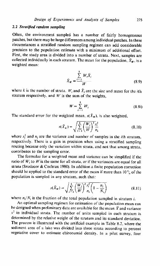
2.2 Stratified random sampling
Often, the environment sampled has a number of fairly homogeneous
patches, but there may be large differences among individual patches. In these
circumstances a stratified random sampling regimen can add considerable
precision to the population estimate with a minimum of additional effort.
First, the study area is divided into a number of strata. Next, samples are
collected individually in each stratum. The mean for the population, Xw> is a
weighted mean:
where k is the number of strata. W{ and X-, are the size and mean for the /th
stratum respectively, and W is the sum of the weights,
i= 1
The standard error for the weighted mean, .v(AV), is also weighted.
, (810)where sf and «, are the variance and number of samples in the /th stratum.
respectively. There is a gain in precision when using a stratified sampling
routing because only the variation within strata, and not that among strata,
contributes to the sampling error.
The formulae for a weighted mean and variance can be simplified if the
ratio of W-, to W is the same for all strata, or if the variances are equal for all
strata (Snedecor & Cochran 1980). In addition a finite population correction
should be applied to the standard error of the mean if more than 10 % of the
population is sampled in any stratum, such that:
where /?,/A', is the fraction of the total population sampled in stratum /.
An optimal sampling regimen for estimation of the population mean can
be designed when preliminary data are available for the mean A" and variance
.v2 in individual strata. The number of units sampled in each stratum is
determined by the relative weight of the stratum and its standard deviation.
The process is illustrated with the artificial example in Table 8.2, where the
sediment area of a lake was divided into three strata according to percent
vegetative cover to estimate chironomid density. In a pilot survey, four

276 Chapter 8
8.2 Example to illustrate the technique of stratified random sampling.
Number of chironomids (cm ~2) in four random samples collected in each of three
strata, A, B, and C with vegetative cover over >75%, <75% & >50%, and
<50% of the area, respectively. The zones represent 20, 30, and 50 x l02m2,
respectively.
x,
4
i = 1
4
IX?i= 1
W,
w1
w
A
50
40
60
30
45
180
8600
166-67
20
0-2
Stratum
B
20
15
25
20
20
80
1650
16-667
30
0-3
C
5
6
9
2
5-5
22
146
8-333
50
0-5
samples were collected in each stratum. A quick inspection of the data shows
that the density estimates in section A are much more variable than in either
sections B or C. A weighted mean (XiV) and standard deviation of the weighted
mean (.v(AV)) are calculated following equations 8.9 and 8.10:
_ 20(45)+ 30(20)+ 50(5-5)
Xw-~- ioo
= 17-75
and
= 1 -6 chironomids cm ~2
A decision can then be made about the total number of samples to be
collected. The sampling fraction in each stratum should be proportional to the
weight W{ and standard deviation .v, in each stratum. As illustrated in Table
8.3, a weighted standard deviation W^.v, is calculated for each stratum. These

Design of Experiments and Analysis of Samples 111
Table 8.3. Calculations for obtaining the optimum sample size of individual strata.
The calculations are based on data from Table 8.2.
Stratum
A
B
C
Total
Surface area
represented
(xl02m2)
20
30
50
100
Mean number
chironomids
(cm"2)
45
20
5-5
Standard
deviation
Si
12-91
4082
2-887
Wisi
258-2
122-5
144-4
525-1
Relative
sample
size
0-4917
0-2333
0-2750
10000
Actual
sample
size
59
28
33
120
values are then summed over all strata. The relative sample size for each
stratum is the ratio of W;S; to £{==, W$t. As a consequence of the high standard
deviation(s) in stratum A, the relative size of this sample is 49 %, or more than
twice its relative weight WJW. If, for example, the total sample size was 120
samples then the optimum sampling programme would be to collect 59
samples in stratum A, as opposed to 24 samples based on proportional
representation alone. The sampling strategy which collects a number of
samples in each stratum proportional to the product of the weight and the
standard deviation of the stratum reduces the standard error. Thus, if it is
assumed that the sample variance (s2) is a good estimate of the population
variance (<r2) in the example in Table 8.3. then the weighted standard error of
the mean is 25% lower with the optimal as opposed to a proportional
sampling regimen (i.e.. s(Xw) = Q-4$ as compared to 0-60). Various
modifications of the randomized stratified sampling method are described by
Stuart (1962) and Cochran (1977).
2.3 Systematic sampling
Systematic samples are evenly spaced throughout a designated area with the
initial sampling point chosen randomly. For example, a random point was
chosen on a small lake and samples were collected at that point and at five
points 0-2 km apart in a westerly direction. Systematic sampling is more even
than random sampling and easier to set up. It is often used for plankton
samples when individual samples are pooled. It does, however, have two
disadvantages over the random sample: it is not accurate if there is a
periodicity over the same distance as the interval between samples. In
addition, there is no general formula to estimate standard error, although
there are formulae for some situations (e.g., Cochran 1977).

278 Chapter 8
2.4 Ratio and regression estimates
The ratio estimate is another way ofestimating population size. It is used when
the size X of one population is known, the size Y of a second population is
unknown, and the ratio of Y to X, R, is known. The information sought is the
size of Y. The parameters X and Y could be the same population in two
different years. If the mean rather than total numbers are of interest, then X
and Kare replaced by ^and Y, respectively. The value of Yis estimated from:
Y = RX (8.12)
The ratio estimate is designed for situations where /?, the ratio of Y to X, is
relatively constant over the study population. For example, suppose there was
a constant ratio of mean zooplankton (?) to mean phytoplankton (X)
biomass in a group of lakes. If, in one of these lakes, the phytoplankton but
not the zooplankton biomass has been measured the ratio estimate could be
used to predict the standing crop of zooplankton. The method ofcalculating a
standard error for Y is described in Snedecor & Cochran (1980).
Sometimes the ratio of Y to X is not constant, but a straight line
relationship appears to exist between them, i.e., there is a linear relationship
with a non-zero intercept. In this case a regression estimate is appropriate (see
Section 5.1). This technique is described in Cochran (1977). Both the ratio and
regression estimations are useful for survey information, although infor
mation on distribution is lost.
2.5 Gradients in space
Vertical and horizontal gradients in planktonic and benthic organisms must
be considered when designing a sampling routine. Since there are so few
studies in the literature, pilot surveys (see Section 2.1.2) on the extent ofspatial
gradients in the population become an invaluable tool. From papers which
have published data on spatial variation in plankton it is clear that the
variation over a whole lake is greater than at a single location, as illustrated in
Table 8.1.
2.6 Composite samples
Aquatic biologists often collect several samples to estimate one parameter,
these samples being pooled to create a composite sample. Although
information on spatial variation is lost in composite samples, this process is
often necessary when it is not feasible to analyze all of the individual samples.
The sampling programme for composite samples should take into account the
natural variation in the community. Samples may be pooled along the main
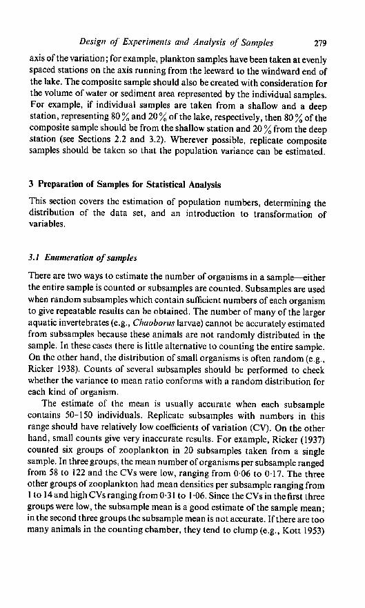
Design of Experiments and Analysis of Samples 279
axis of the variation; for example, plankton samples have been taken at evenly
spaced stations on the axis running from the leeward to the windward end of
the lake. The composite sample should also be created with consideration for
the volume of water or sediment area represented by the individual samples.
For example, if individual samples are taken from a shallow and a deep
station, representing 80 % and 20 % of the lake, respectively, then 80 % of the
composite sample should be from the shallow station and 20 % from the deep
station (see Sections 2.2 and 3.2). Wherever possible, replicate composite
samples should be taken so that the population variance can be estimated.
3 Preparation of Samples for Statistical Analysis
This section covers the estimation of population numbers, determining the
distribution of the data set, and an introduction to transformation of
variables.
3.1 Enumeration of samples
There are two ways to estimate the number of organisms in a sample—either
the entire sample is counted or subsamples are counted. Subsamples are used
when random subsamples which contain sufficient numbers of each organism
to give repeatable results can be obtained. The number of many of the larger
aquatic invertebrates (e.g., Chaoborus larvae) cannot be accurately estimated
from subsamples because these animals are not randomly distributed in the
sample. In these cases there is little alternative to counting the entire sample.
On the other hand, the distribution of small organisms is often random (e.g.,
Ricker 1938). Counts of several subsamples should be performed to check
whether the variance to mean ratio conforms with a random distribution for
each kind of organism.
The estimate of the mean is usually accurate when each subsample
contains 50-150 individuals. Replicate subsamples with numbers in this
range should have relatively low coefficients of variation (CV). On the other
hand, small counts give very inaccurate results. For example, Ricker (1937)
counted six groups of zooplankton in 20 subsamples taken from a single
sample. In three groups, the mean number of organisms per subsample ranged
from 58 to 122 and the CVs were low, ranging from 006 to 017. The three
other groups of zooplankton had mean densities per subsample ranging from
1 to 14 and high CVs ranging from 0-31 to 1 06. Since the CVs in the first three
groups were low, the subsample mean is a good estimate of the sample mean;
in the second three groups the subsample mean is not accurate. If there are too
many animals in the counting chamber, they tend to clump (e.g., Kott 1953)
280 Chapter 8
and the counts may also be inaccurate. See Chapter 7 for a fuller treatment of
sample enumeration and its implications.
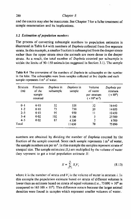
3.2 Estimation ofpopulation numbers
The process of converting subsample numbers to population estimates is
illustrated in Table 8.4 with numbers of Daphnia collected from five separate
strata. In this example, a smaller fraction is subsampled from the deeper strata
rather than the upper strata since the animals are more dense in the deeper
strata. As a result, the total number of Daphnia counted per subsample is
within the limits of 50-150 animals (as suggested in Section 3.1). The sample
Table 8.4 The conversion of the numbers of Daphnia in subsamples to the number
in the lake. The subsamples were from samples collected at five depths and each
sample represents 1 m3 of water.
Stratum
(m)
0-1
1-2
2-3
3-4
4-5
Total
Fraction
of the
sample
counted
010
010
010
002
002
Daphnia in
subsample
52
73
95
102
87
Daphnia in
sample
520
730
950
5 100
4350
11650
Volume
of water
per stratum
(xl06m3)
32
20
11
5
2
70
Daphnia per
stratum
(xlO6)
16640
14600
10450
25 500
8 700
75 890
numbers are obtained by dividing the number of Daphnia counted by the
fraction of the sample counted. Since each sample represents 1 m3 of water,
the sample numbers are per m3. In this example the samples represent strata of
unequal size. The sample estimates (A',) are multiplied by the volume of water
they represent to get a total population estimate X:
(8.13)i= 1
where k is the number of strata and Vx is the volume of water in stratum /. In
this example the population estimate based on strata of different volumes is
lower than an estimate based on strata of equal volumes (i.e., 75 890 x 106 as
compared to 163 100 x 106). This difference occurs because the larger animal
densities were found in samples which represent smaller volumes of water.

Design of Experiments and Analysis of Samples 281
3.3 Smoothing data
Estimates of changes in the number of aquatic organisms over time are often
relatively imprecise because of inadequate sampling. When looking for trends
with time, smoothing of population numbers is recommended (e.g.,
Edmondson 1960; covered in detail in Tukey 1977). Smoothing involves
replacing population estimates on individual dates by moving averages,
usually from three or five consecutive dates. If population estimates for three
consecutive dates are X^ ,. X{ and XH ,. then the three-date moving average
X{ is:
— jt£ ; — i "T" *\ ; i ^l; a. iX. = -LJ. _i LLL (8 14)
The number of dates included in moving averages should be inversely related
to the confidence which is placed in individual population estimates. In Table
8.5, population estimates prior to smoothing and three- and five-week running
averages are presented. In this example, smoothing eliminates the small
fluctuation in population numbers between the third and seventh weeks and
reduces the peak value recorded for the ninth week. Smoothing reduces the
possibility of attributing causes to short-term population fluctuations which
are the result of sampling inadequacies. On the other hand, some information
on short- term change is lost, and erroneous conclusions can be drawn from
moving averages (e.g. Cole 1954, 1957).
Table 8.5 An example to illustrate smoothing of data.
Week
i
1
2
3
4
5
6
7
8
9
10
11
12
Observed
population numbersvA,
76
90
86
105
117
106
130
150
500
140
120
98
Running
X
3 week
84
94
103
109
118
129
260
263
253
119
average
5 week
95
101
109
122
201
205
208
202
282 Chapter 8
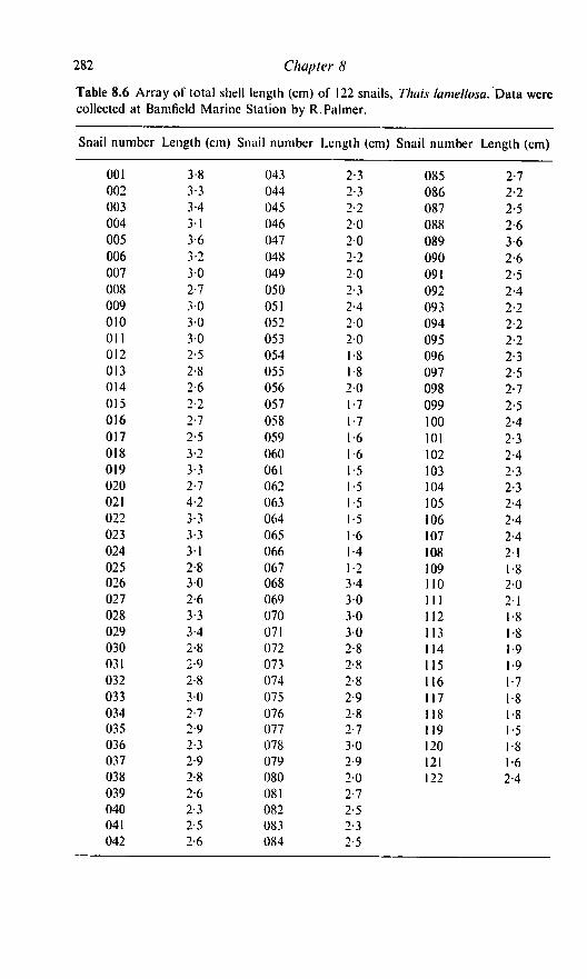
Table 8.6 Array of total shell length (cm) of 122 snails, Thais lamellosa. Data were
collected at Bamfield Marine Station by R.Palmer.
Snail number
001
002
003
004
005
006
007
008
009
010
011
012
013
014
015
016
017
018
019
020
021
022
023
024
025
026
027
028
029
030
031
032
033
034
035
036
037
038
039
040
041
042
Length (cm)
3-8
3-3
3-4
3-1
3-6
3-2
30
2-7
30
30
3-0
2-5
2-8
2-6
2-2
2-7
2-5
3-2
3-3
2-7
4-2
3-3
3-3
31
2-8
3-0
2-6
3-3
3-4
2-8
2-9
2-8
30
2-7
2-9
2-3
2-9
2-8
2-6
2-3
2-5
2-6
Snail number
043
044
045
046
047
048
049
050
051
052
053
054
055
056
057
058
059
060
061
062
063
064
065
066
067
068
069
070
071
072
073
074
075
076
077
078
079
080
081
082
083
084
Length (cm)
2-3
2-3
2-2
2-0
20
2-2
20
2-3
2-4
20
20
:
•8
1-8
2-0
•7
■7
■6
■6
•5
■5
■5
•5
•6
•4
•2
3-4
30
30
30
2-8
2-8
2-8
2-9
2-8
2-7
3-0
2-9
20
2-7
2-5
2-3
2-5
Snail number
085
086
087
088
089
090
091
092
093
094
095
096
097
098
099
100
101
102
103
104
105
106
107
108
109
110
111
112
113
114
115
116
117
118
119
120
121
122
Length (cm)
2-7
2-2
2-5
2-6
3-6
2-6
2-5
2-4
2-2
2-2
2-2
2-3
2-5
2-7
2-5
2-4
2-3
2-4
2-3
2-3
2-4
2-4
2-4
21
1-8
2-0
2-1
1-8
•8
•9
■9
■7
•8
•8
•5
•8
■6
2-4
Design of Experiments and Analysis ofSamples 283
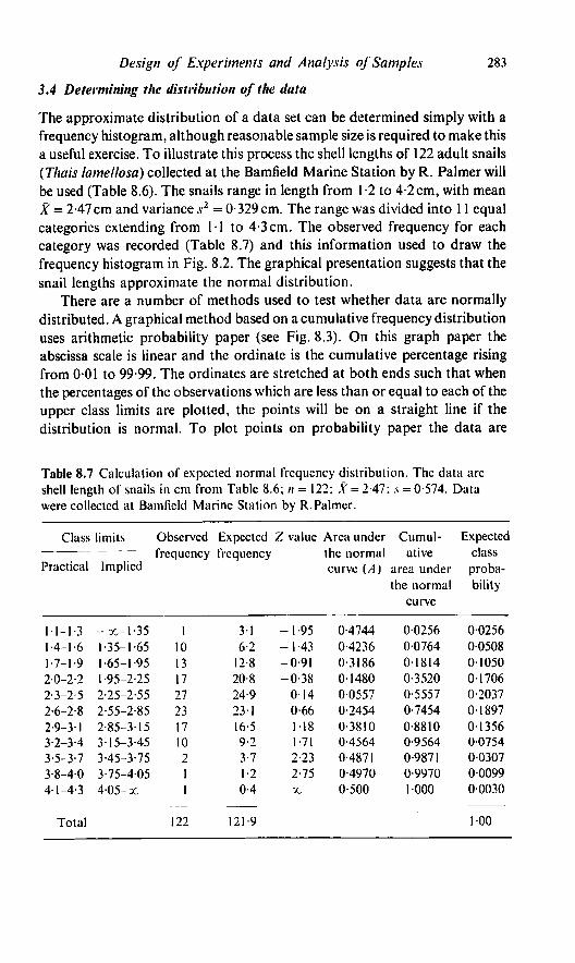
3.4 Determining the distribution of the data
The approximate distribution of a data set can be determined simply with a
frequency histogram, although reasonable sample size is required to make this
a useful exercise. To illustrate this process the shell lengths of 122 adult snails
(Thais lamellosa) collected at the Bamfield Marine Station by R. Palmer will
be used (Table 8.6). The snails range in length from 1 -2 to 4-2cm, with mean
X = 2-47 cm and variance .v2 = 0-329 cm. The range was divided into 11 equal
categories extending from 11 to 4-3 cm. The observed frequency for each
category was recorded (Table 8.7) and this information used to draw the
frequency histogram in Fig. 8.2. The graphical presentation suggests that the
snail lengths approximate the normal distribution.
There are a number of methods used to test whether data are normally
distributed. A graphical method based on a cumulative frequency distribution
uses arithmetic probability paper (see Fig. 8.3). On this graph paper the
abscissa scale is linear and the ordinate is the cumulative percentage rising
from 001 to 99-99. The ordinates are stretched at both ends such that when
the percentages of the observations which are less than or equal to each of the
upper class limits are plotted, the points will be on a straight line if the
distribution is normal. To plot points on probability paper the data are
Table 8.7 Calculation of expected normal frequency distribution. The data are
shell length of snails in cm from Table 8.6; n = 122; X = 2-47; s = 0-574. Data
were collected at Bamfield Marine Station by R. Palmer.
Class
Practical
1-1-1-3
1-4-1-6
1-7-1-9
2-0-2-2
2-3-2-5
2-6-2-8
2-9-3-1
3-2-3-4
3-5-3-7
3-8-4-0
4-1-4-3
Total
limits
Implied
-x-1-35
1-35-1-65
1-65-1-95
1-95-2-25
2-25-2-55
2-55-2-85
2-85-3-15
3-15-3-45
3-45-3-75
3-75-4-05
405-x
Observed
frequency
1
10
13
17
27
23
17
10
2
1
1
122
Expected
frequency
31
6-2
12 8
20-8
24-9
23-1
16-5
9-2
3-7
1-2
0-4
121-9
Z value
-1-95
-1-43
-0-91
-0-38
014
0-66
118
1-71
2-23
2-75
X
Area under
the normal
curve {A)
0-4744
0-4236
0-3186
01480
0-0557
0-2454
0-3810
0-4564
0-4871
0-4970
0-500
Cumul
ative
area under
the normal
curve
00256
00764
01814
0-3520
0-5557
0-7454
0-8810
0-9564
0-9871
0-9970
1000
Expected
class
proba
bility
00256
00508
01050
01706
0-2037
0-1897
01356
0-0754
00307
00099
00030
100

284 Chapter 8
30
20
10
1.05 1.65 2.25 2.85 3.45
Shell length of snails (cm)
4.05
Fig. 8.2 Histogram of total shell length of 122 snails, Thais lamellosa. The dashed
curve is the normal distribution with mean /< = 2-47 and variance a2 = 0-329.
Data were collected at Bamfield Marine Station by R.Palmer.
divided into equal size classes, the frequency is calculated for each class, and
the cumulative frequency is plotted against the upper class limit. A straight
line is drawn by hand through the points, giving most weight to the points
between the cumulative frequencies of 25 % to 75 %. This method is illustrated
in Fig. 8.3 using the snail data from Table 8.8. The points in Fig. 8.3 fall close
to a straight line and thus appear to be normally distributed, as they were in
Fig. 8.2. This method works well for large samples («>60); however, for
small samples, a more suitable graphical test for normality of a frequency
distribution is the Rankit method. Both of these graphical methods are for
continuous data and are described in Cassie (1963) and Sokal & Rohlf(1981).
Another approach to determine whether data follow a normal distribution
is to calculate the theoretical or expected distribution and compare this with
the observed distribution—this is suitable for large samples sizes. It will be
illustrated with the calculation of an expected normal frequency distribution

Design of Experiments and Analysis of Samples 285
99.9
99.8
99.5
99
98
«■ 95
8« 90
1 80
1 70B 60
c 50
2 40
§. 30
•1 20
1 10
5
2
1
0.5
0.2
0.1
/
/
-•
•
/
: S/
V
- /- '
-
-
I I I 1 I 1 I 1
//
/ •
i i i i
1.35 1.95 2.55 3.15 3.75
Shell length of snails (cm)
4.35
Fig. 8.3 Shell length of snails, Thais lamellosa, plotted on probability paper. Data
were collected at Bamfield Marine Station by R.Palmer.
for the snail data (Table 8.7). There are five steps in calculating an expected
normal frequency distribution.
(1) A standard deviation unit or Z value is calculated for each upper class
limit A',,:
Z =x-x
(8.15)
In the example, the first upper class limit is 1-35 cm, the mean (X) and
standard deviation (s) are 2-47 and 0-574cm, respectively, and the Z value is:
1-35-2-47
0-574 ~

286 Chapter 8
Table 8.8 The calculations required to use arithmetic probability paper to test for
normality of a frequency distribution. The data are shell length of snails in cm
from Table 8.7. Data were collected at Banfield Marine Station by R.Palmer.
Class
mean
1-2
1-5
1-8
2-1
2-4
2-7
30
3-3
3-6
3-9
4-2
Total
Upper
class
limit
1 35
1-65
1 95
225
2-55
285
315
3-45
3-75
405
4-35
Observed
frequency
1
10
13
17
27
23
17
10
2
1
1
122
Cumulative
frequency
1
11
24
41
68
91
108
118
120
121
122
Percent
cumulative
frequency
0-82
91
19-7
33-6
55-7
74-6
88-5
96-7
98-4
9918
1000
(2) The area under the normal curve (A) is then read from a table of the
cumulative normal frequency distributions (available in most statisticaltexts).
For example, when Z = 1 -95 (which is the case for the first category in
the snail data) A = 0-4744.
(3) The cumulative area under the curve is calculated for each class as
follows: for negative Z, use (0-5 - A); for positive Z, use (0-5 + A). The
cumulative area under the portion of the curve extending from - x to
1 -35 cm is thus (0-5 - 0-4744) = 00256.
(4) The expected class probabilities are calculated by subtracting successive
cumulative probabilities. For the first category in the snail data (- oc to
1 -35cm) the expected class probability is (00256-0) = 0-0256.
(5) To obtain the expected frequencies, the class probabilities are multiplied
by the sample size, which is 122 in the example used here.
For the snail data the expected frequencies appear similar to the observed
frequencies (Table 8.7). To test whether the observed distribution fits the
expected distribution, the *2-test is normally applied (see Section 3.5.1).
Alternatively, when the sample size is small the Kolmogorov-Smirnov test for
goodness-of-fit should be applied because it is more powerful (see Sokal &
Rohlf 1981).
Design of Experiments and Analysis of Samples 287
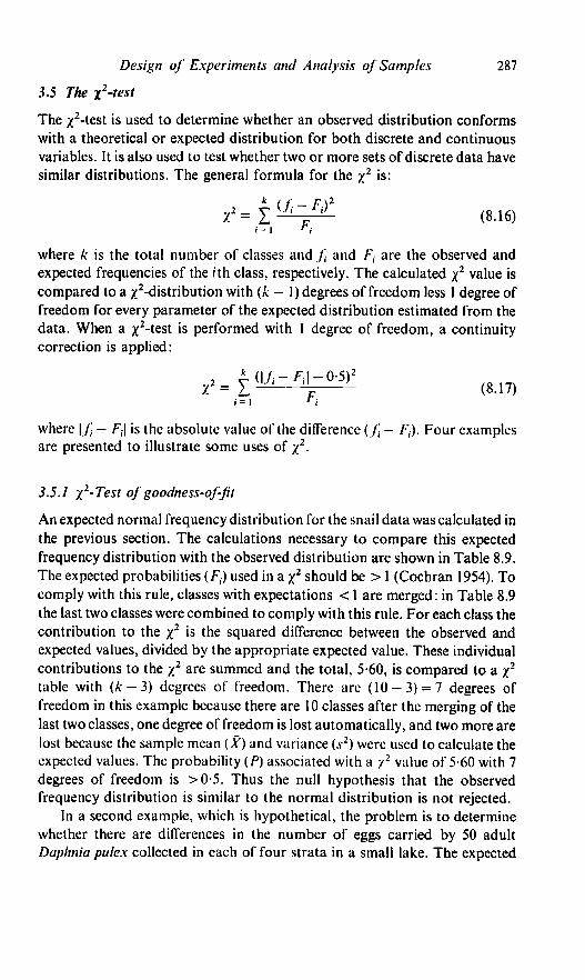
3.5 The y>2-test
The x2-test is used to determine whether an observed distribution conforms
with a theoretical or expected distribution for both discrete and continuous
variables. It is also used to test whether two or more sets of discrete data have
similar distributions. The general formula for the y2 is:
k ( f _ f)2
y.2 = I Jl1tiL (8-i6)i=i ti
where k is the total number of classes and j\ and F, are the observed and
expected frequencies of the rth class, respectively. The calculated y2 value is
compared to a ^-distribution with (k — 1) degrees of freedom less 1 degree of
freedom for every parameter of the expected distribution estimated from the
data. When a yz-test is performed with 1 degree of freedom, a continuity
correction is applied:
, * (l/i-F.I-0-5)2
where | /■ - Fs\ is the absolute value of the difference (j\ - F{). Four examples
are presented to illustrate some uses of y2.
3.5.1 y2-Test of goodness-of-fit
An expected normal frequency distribution for the snail data was calculated in
the previous section. The calculations necessary to compare this expected
frequency distribution with the observed distribution are shown in Table 8.9.
The expected probabilities (F{) used in a y2 should be > 1 (Cochran 1954). To
comply with this rule, classes with expectations < 1 are merged: in Table 8.9
the last two classes were combined to comply with this rule. For each class the
contribution to the y2 is the squared difference between the observed and
expected values, divided by the appropriate expected value. These individual
contributions to the y2 are summed and the total, 5-60, is compared to a y2
table with (A—3) degrees of freedom. There are (10 —3) = 7 degrees of
freedom in this example because there are 10 classes after the merging of the
last two classes, one degree of freedom is lost automatically, and two more are
lost because the sample mean (X) and variance (.v2) were used to calculate the
expected values. The probability (P) associated with a y2 value of 5-60 with 7
degrees of freedom is >0-5. Thus the null hypothesis that the observed
frequency distribution is similar to the normal distribution is not rejected.
In a second example, which is hypothetical, the problem is to determine
whether there are differences in the number of eggs carried by 50 adult
Daphnia pulex collected in each of four strata in a small lake. The expected

288 Chapter 8
Table 8.9 The x2 goodness-of-fit test. The observed frequencies of snail shell
lengths are from Table 8.7 and the expected frequencies are calculated assuming a
normal frequency distribution.
Class
mean
1-2
1-5
1-8
2.1
2-4
2-7
3-0
3-3
3-6
3-9
4-2
Total
Observed
frequency
(/)
1
10
13
17
27
23
17
10
2
!} 2122
Expected
frequency
(F)
31
6-2
12 8
20-8
24-9
23-1
16-5
9-2
3-7
121-9
f-F
-21
3-8
0-2
-3-8
21
-01
0-5
0-8
-1-7
0-4
Contribution
to*2
1-42
234
000
0-69
018
000
0-02
007
0-78
010
5-60
frequency for each stratum is the total number of observations divided by the
number of strata, as illustrated in Table 8.10. The expected frequency was
computed on the basis of the expected ratio of 1:1:1:1. This expected ratio is
extrinsic to the sampled data and thus no additional degrees of freedom are
lost. The x2 value of 11 -58 is compared to a ^-distribution with 3 degrees of
freedom. Since the calculated x2 value has a P < 0-01, the data are not
consistent with the null hypothesis that the distribution of Daphnia eggs in the
four strata is homogeneous.
Table 8.10 The x2 goodness-of-fit test where the hypothesis is extrinsic to the
sampled data. The data are number of eggs carried by 50 adult Daphnia pulex
selected randomly from samples collected in each of four strata in a lake.
Stratum
1
2
3
4
Total
Observed
frequency
</>
106
83
75
64
328
Expected
frequency
(F)
82
82
82
82
328
f-F
24
1
-7
-18
Contribution
to x2
702
001
0-60
3-95
11-58
Design of Experiments and Analysis of Samples 289
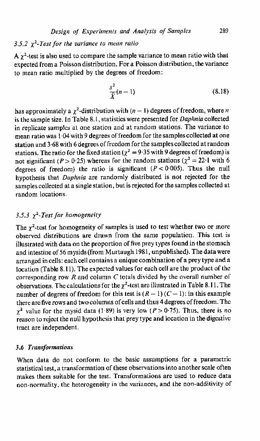
3.5.2 x1-Test for the variance to mean ratio
A x2-test is also used to compare the sample variance to mean ratio with that
expected from a Poisson distribution. Fora Poisson distribution, the variance
to mean ratio multiplied by the degrees of freedom:
*2(8.18)
has approximately a ^-distribution with (« - 1) degrees of freedom, where n
is the sample size. In Table 8.1, statistics were presented for Daphnia collected
in replicate samples at one station and at random stations. The variance to
mean ratio was 1 04 with 9 degrees of freedom for the samples collected at one
station and 3-68 with 6 degrees offreedom for the samples collected at random
stations. The ratio for the fixed station (/2 =935 with 9 degrees of freedom) is
not significant (P > 0-25) whereas for the random stations (#2 = 22-1 with 6
degrees of freedom) the ratio is significant (/*< 0-005). Thus the null
hypothesis that Daphnia are randomly distributed is not rejected for the
samples collected at a single station, but is rejected for the samples collected at
random locations.
3.5.3 yf-Testfor homogeneity
The x2-test for homogeneity of samples is used to test whether two or more
observed distributions are drawn from the same population. This test is
illustrated with data on the proportion of five prey types found in the stomach
and intestine of 56 mysids (from Murtaugh 1981, unpublished). The data were
arranged in cells: each cell contains a unique combination of a prey type and a
location (Table 8.11). The expected values for each cell are the product of the
corresponding row R and column C totals divided by the overall number of
observations. The calculations for the x2-test are illustrated in Table 8.11. The
number of degrees of freedom for this test is (R - 1) (C - 1): in this example
there are five rows and two columns of cells and thus 4 degrees of freedom. The
X2 value for the mysid data (1-89) is very low (/>>0-75). Thus, there is no
reason to reject the null hypothesis that prey type and location in the digestive
tract are independent.
3.6 Transformations
When data do not conform to the basic assumptions for a parametric
statistical test, a transformation of these observations into another scale often
makes them suitable for the test. Transformations are used to reduce data
non-normality, the heterogeneity in the variances, and the non-additivity of

290 Chapter 8
Table 8.11 The x2 test for homogeneity of sampfes. The observed and expected
frequencies are for the numbers of various groups of planktonic organisms in the
digestive tract of the predator Neomysis mercedis. Data are from P.A.Murtaugh
(1981, unpublished).
Prey
type
Daplmia
Calanoid copepods
Cylopoid copepods
Rotifers
Other (e.g. Bosmina)
Column total
Daphnia
Calanoid copepods
Cylopoid copepods
Rotifers
Others (e.g. Bosmina)
2 ^Ui-fy (452
Location
Stomach
Observed
452
41
28
51
5
577
expected
(577)(554)
Intestine
numbers/
102
9
3
9
1
124
numbers F
(»24)(554) __
701 456 701
41-2 8-84
25-5 5-48
49-4 10-6
4-94 106
-456)2 (41-41-2)2 _ (1-106)2
456 ' 41-2 1-06
Row
total
554
50
31
60
6
701
the treatment effects. A transformation involves taking each observation X{
and converting it to a new number, X\, which is then used in subsequent
calculations. Three commonly used transformations, the logarithmic, the
square root, and the arcsine, will be discussed in this section.
Once a transformation has been applied, the data should be rechecked to
determine whether the transformation has corrected the problem. Several
methods have been developed to determine the best transformation, such as
the Box and Cox (1964) method for non-normal data (described briefly in
Sokal & Rohlf 1981), Taylor's (1961) method for variance stabilization and
Tukey's (1949) method for non-additivity (described in Snedecor & Cochran
1980). One of these, Taylor's method for variance stabilization, will also be
discussed below.

Design of Experiments and Analysis of Samples 291
3.6.1 Logarithmic transformation
This is the most commonly used transformation for biological data, and there
are two forms: logs to the base 10 and natural logarithms, i.e.
X't = \ogl0(X} (8.19)and
X\ = \o^{Xb (8.19i)
respectively. If there are very small numbers or zeros then the transformation
is applied to (X( + 1) instead of Xt. The logarithmic transformation is
illustrated in Section 5.1.1.
3.6.2 Square root transformation
The square root transformation:
/ (8.20)
is normally applied to data that follow the Poisson distribution. If there are
zero values, then the transformation:
/0-5 (8.20i)
is applied (e.g., Kutkuhn 1958).
3.6.3 Arcsine transformation
Data which are expressed as percentages or proportions and lie between
0-30% and 70-100 % are usually non-normal, i.e., there are too many values
at the tails of the distribution relative to the centre. The arcsine or angular
transformation:
X\ = arcsin VO^ (8.21)
reduces the scale in the middle of a distribution and extends the tails.
3.6.4 Taylor's methodfor variance stabilization
Taylor (1961) showed that, for data on the abundance of organisms, there is a
simple power law relationship between the variance (s2) and the mean (X):
s2=aXh (8.22)
Where a and b are parameters describing the study population, and that the
appropriate transformation is:
X; = Xj-°-5h (8-23)
X'i = (Xi + c)1-°-5b (8.23i)

292 Chapter 8
where c is a constant such as 0-5 or 1 and b is the coefficient from equation
8.22. When b = 0, the distribution is regular and no transformation is
necessary. The distribution is Poisson and a square root transformation
(^/X = X0'5) is suggested when 6=1. A logarithmic transformation isrecommended when b = 2, and when b > 2 a negative power function is the
appropriate transformation.
Taylor's method is useful only for cases where numerous estimates ofthe fi
and a2 can be collected. Downing (1979) gathered enough data to examine the
relationship between the mean and variance for benthic invertebrates that
were collected with several types of samplers and from various substrates. He
found that a fourth root transformation was the most appropriate for the
samples examined. Further investigations are required to determine the
general applicability of Downing's fourth root transformation to data on the
abundance of aquatic invertebrates (Taylor 1980).
4 Comparison of Means and Related Topics
This section focuses on the /-test as a method for comparing two or more
means. Alternatives to the standard Mests are also introduced, although the
most important alternative, the analysis of variance (ANOVA), is discussed
only briefly. A test for combining probabilities from independent tests of
significance is considered in this section. Since most statistical tests for the
comparison of means assume that the sample variances are homogeneous,
three tests for homogeneity of sample variances are also reviewed.
4.1 Calculation of an average variance and tests for homogeneity of sample
variance
An estimate of average variance is required for most Mests. If there are A:
independent estimates (s2. s22 .vj~) of the same population variance a2, with
(/?i - 1), («2-l) (w*-0 degrees of freedom, respectively, a single
estimate of a1 is given by the weighted average of sample variances:
(8.24)
i= 1
The calculation of an average variance is illustrated in Table 8.12 with data
from Peters & Rigler (1973) on the reproductive rate of adult Dapfmia fed
three different concentrations of yeast.
This calculation of an average variance (equation 8.24) assumes that the
estimated variances are consistent with one another. Three ways to test
whether the variances are homogeneous will be outlined.
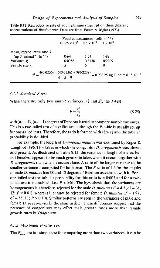
Design of Experiments and Analysis of Samples 293
Table 8.12 Reproductive rate of adult Daphnia rosea fed on three different
concentrations of Rhodotorula. Data are from Peters & Rigler (1973).
Food concentration (cells ml"')
0125 x 105 0-5 x 10s 1 x 10⁵
Mean, reproductive rate X-,
(ng P animal"1 hr"1) 0-64 1-74 1-89
Variance^ 00256 0-3136 0-2209
Sample size ;i, 5 6 10
, 4(0-0256)+5(0-3136)+9(0-2209) n n „, . , . .s2 = —7—-—j- = 0-203 25 ng P animal"' hr"l
4 + 5+9
4.1.1 Standard F-test
When there are only two sample variances, .vf and s\s the F-test
with («, — 1). («2 — I) degrees of freedom is used to compare sample variances.
This is a two-tailed test of significance, although the F-table is usually set up
for one-tailed tests. Therefore, the ratio is formed with s\ > s\ and the tabular
probability is doubled.
For example, the length of Diaptomus minutus was examined by Rigler &
Langford (1967) for lakes in which the congenitor D. oregonensis was absent
and present. As illustrated in Table 8.13, the variance in length of males, but
not females, appears to be much greater in lakes when it occurs together with
D. oregonensis than when it occurs alone. A ratio of the larger variance to the
smaller variance is computed for both sexes. The F-ratio of 4-5 for the lengths
of male D. minutus has 38 and 12 degrees of freedom associated with it. For a
one-tailed test the tabular probability for this ratio is < 0-005 and for a two-
tailed test it is doubled, i.e., P<001. The hypothesis that the variances are
homogeneous is, therefore, rejected for the male D. minutus (F= 4-5; df = 38,
12; /)<0-01), whereas it cannot be rejected for female D. minutus (F= 1 -97;
df = 35, 13; P > 0-10). Similar patterns are seen in the variances of male and
female D. oregonensis in the same article. These differences suggest that the
presence of congenitors may effect male growth rates more than female
growth rates in Diaptomus.
4.1.2 Maximum F-ratio Test
The Fmax-test is a simple test for comparing more than two variances. It can be

294 Chapter 8
Table 8.13 Total length (mm) of Diaptomus minutus in lakes in which the
congenitor D. oregonensis was absent and present. Data are from Rigler &
Langford 1967).
Males Females
Alone Together Alone Together
Mean X;
Variance s?
Sample size /?,-
s2ln,
0-92 1-01
000105 000472
13 39
000008 000012
100 108
0003 58 000706
14 36
F-test for homogeneity of variances
/•"-ratio0-004 72
= 4-5**000706
= 1-97
freedom df
Probability P
000105 0003 58
38,12 35,13
(<0005 x 2) = <001 (>0-05 x 2)= >010
used when there are up to six variances, all based on the same number of
degrees of freedom. For this test the ratio:
max(.y2)
Fmax minCs2' (8.26)
is formed. This value cannot be compared to the standard F-table which can
be used to compare only two variances at a time; there are tables available,
however, which make proper allowance for the selection of extremes (David
1952; reproduced as Table 17 from Rohlf & Sokal 1981).
The data in Table 8.14 (from Kott 1953) are used to illustrate this test. In
an investigation of an apparatus for subsampling a cladoceran species based
on three separate plankton hauls, the maximum variance was 400-3 animals
Table 8.14 Variances in number of the cladoceran Penilia smaekeri in subsamples
collected with a modified whirling apparatus from three separate plankton hauls.
Data are from Kott (1953).
Haul Number of Sample
subsamples collected variance
10
10
10
92-2
400-3
2900

Design of Experiments and Analysis of Samples 295
per compartment and the minimum variance was 92-2 animals per
compartment. The Fmax value,
F =1 maxmax
for the three variances all with 9 degrees of freedom, is less than the critical
value (P = 005) of 5-34. Thus, heterogeneity of the three sample variances is
not clearly indicated.
4.1.3 Bartleft's test of homogeneity of variances
When there are more than two estimates of variance sf, i.e., k > 2, Bartlett's
test of homogeneity can be applied. This is an approximate z2-test, which, in
most cases, is more efficient than the/^-test. However, the calculations for
Bartlett's test are more extensive and it has been criticized as being too
sensitive to departures from normality in the data. This test requires:
/, = logc sf (8.27)
for each sample variance sf, and:
L = \ogJ2 (8.27i)
from the weighted average variance s2.
The quantity:
M = 17 I "< - ') L - I (»i - ! >'/] (8.27H)can then be compared after correction to the ^-distribution for {k — 1)
degrees of freedom. A correction factor:
C=l1 r * 1 1
.■t-,(fl,-0
is applied to equation 8.27ii because the x2 value tends to be too large. When
the correction is required, M/C is compared with the ^-distribution. C is
always slightly greater than 1 and therefore only needs to be calculated ifM is
slightly larger than the critical y} value.
The data in Table 8.12 on reproductive rates of Daphnia grown in three
different food concentrations are used to illustrate this test. The calculations
are shown in Table 8.15. The M value 5-37 is compared to a ^-distribution
with 2 degrees of freedom. This is a small y2 value for 2 degrees of freedom
(P > 005) and there is, therefore, no reason to assume that the variances are
not homogeneous.

296 Chapter 8
Table 8.15 Bartlett's test for homogeneity of variances. The data are mean
reproductive rate of Daphnia grown in three separate food concentrations (fromTable 8.12). Data are from Peters & Rigler (1973).
Step 1 Calculate /, for each food concentration
Food concentration «,--! sf /, = In .v?(cells ml"1)
0-125 x 10s 4 00256 -3-66516
0-5 x I05 5 0-3136 -115964
1-0 x 105 9 0-2209 -1-51005
Step 2 Calculate L
Since s2 = 0-20325. L = In (020325) = - 1 -59332
Step 3 Calculate M
(i) y («,.- 1)/,-= 4(-3-665 16)+ 5(-1-15964)+ 9(-1-51005)
= -34049 29
Since the average variance .v- is based on 18df
(ii) M= 18(-1-59332)-(-34-04929) = 5.37with A — 1 or 3 — I = 2df
4.2 t-Testfor comparison of a sample mean with the population mean
To determine if a sample mean is significantly different from an assumed
population mean, a /-test is used. The / value is the ratio of the deviation of a
sample mean {X) from the population mean (/<) to the standard error of themean (.Vy).
X-nt= (8.28)
•v.v
This / value is compared with the Student's /-distribution with (// - 1) degrees
of freedom. It is assumed that the sample mean (X) is normally distributed.
This test is illustrated with data from Lampert (1974) in which he
investigated whether filter feeders showed preferences for certain food items.
Daphnia pulex were fed a mixture of labelled bacteria and algae. A coefficient
of selection. S, was calculated to determine to what extent bacteria were
preferred to algae. If there was no food preference the coefficient of selection
would be 5=1. In one experiment with four observations the average
coefficient of selection S was 1-65 and the sample variance .v2 was 00784. In
order to test whether this value of 1 65 (X) is different from 1 (/<), a standard
error of the mean s% is first calculated:
■vv= /—- =0 14

Design of Experiments and Analysis of Samples 297
The / value,
1-65-1
014= 1-8
is compared with the Student's /-distribution with 3 degrees of freedom. Since
the Student's t value for P = 0005 and 3 degrees of freedom is 7-45, the null
hypothesis that Daphnia show no preference for food organisms is rejected.
4.3 Comparison of two independent means
4.3.1 Standard t-test
The standard method for comparison of two independent means, Xx and X2,
is the /-test. This test assumes that:
(1) The observations which are used to calculate Xx and X2 are independent.
(2) The means Xx and X2 are normally distributed.
(3) The variances in the two populations are homogeneous.
This comparison requires the standard error of the difference between two
means:
(8.29)
where s2 is the average variance (see Section 4.1) and n, and n2 are the number
of observations used to compute Xx and X2> respectively. To test whether the
difference between the means is different from zero, the value:
A\ -X,t = — - (8.29i)
SX, - AS
is calculated and compared to a Student's /-table with (n, + n2 - 2) degrees of
freedom.
The standard /-test is illustrated with mean length data for female D.
minutus when they occur alone and with a congenitor (Table 8.13). There are
three calculations required: from equation 8.24, an average variance:
_2 13(000358)+ 35(000706)jt = — = 000612 mm
48
from equation 8.29, a standard error of the difference between the means:
sXl.S2= /0-006 12 (A + i)= 002464mm

298 Chapter 8
and finally the value:
1 00-1 08/ = = 3-25
002464
This / value is compared with a two-tailed /-distribution with 48 degrees of
freedom. Since the probability is <0-005, the hypothesis that the mean length
of female D. minutus is unaffected by the presence ofthe congenitor is rejected.
4.3.2 t-Test for samples with heterogeneous variances
The standard /-test makes the assumption that the sample variances are
homogeneous. When this assumption does not hold the investigator has two
choices—either transform the variables to reduce the heterogeneity or use a
modified /-test to compare the means. If the variances are heterogeneous, a
standard /-test is not accurate: the null hypothesis will be rejected too few
times if the larger sample has the larger variance and too many times if the
larger sample has the smaller variance. If heterogeneity of variances is
suspected and is not corrected by a transformation of the data, the standard
/-test must be modified so that the / value will approximate a /-distribution
(Snedecor & Cochran 1980). A weighted variance is not used to calculate the
standard error of the mean s'Xl - .?„ rather:
(8.30)V"l "2
and:
f =—, (8.3Oi)SA'l - Xl
where Xx and X2% s* and .vf. and /;, and n2 are the means, variances and sample
size for the first and second samples, respectively. The degrees of freedom are
also modified:
df TV* ^~T (8J1)
The /' value is then compared with the Student's /-distribution with df' degrees
of freedom.
This test is illustrated with a comparison of the mean lengths of male D.
minutus in the presence and absence of a congenitor. The variances for this

Design of Experiments and Analysis of Samples 299
example are heterogeneous (Table 8.13). This /-test requires a standard error
of the differences between two means:
.<?, _ jp2 = ^0-00008+ 0000 12 = 0-014 14 mm
a /' value:
and degrees of freedom:
(0-00008 +0000 12):
/(000008)2 (0-00012)2
V 12 + 38
= 44
The sign of the /' value is ignored and it is compared with a Student's
/-distribution with 44 degrees of freedom. This /' value is highly significant
(P < 0001) and thus the hypothesis that the mean length of male D. minutus is
unaffected by the presence of the congenitor is rejected. Calculations for the
standard /-test would result in a / value of 4-53 with 50 degrees of freedom.
Both of these values would be incorrect, although, for this example, the same
conclusions would be drawn.
4.3.3 Nonparametric alternative to the t-test
In cases where the distribution of the samples is unknown or the data cannot
be transformed to approximate the normal distribution, a nonparametric
alternative is recommended. Nonparametric tests make fewer assumptions
than standard tests; for example, there are no assumptions about the
distribution of the data nor of variance homogeneity. However, these tests
tend to be less powerful than their parametric alternatives, especially when the
sample size is small.
The Mann-Whitney or Wilcoxon rank sum test is a nonparametric
alternative to the standard /-test. As in many nonparametric tests, the first step
is to rank the data. The ranks are then summed for each sample and the results
compared with specially prepared tables. Additional calculations are required
when the sample sizes are not equal and when the sample size is outside the
limits of the table (e.g., Conover 1980; Snedecor & Cochran 1980; Sokal &
Rohlf 1981). This test is illustrated with data from Grant & Bayly (1981) which
are reproduced in Table 8.16. They investigated the effect ofcrest development
in cladocerans on their vulnerability to predation. These data are expressed as
percentages and, as a result, may not be normally distributed. Thus, it is
appropriate to use a nonparametric test to determine whether there are
differences between the vulnerability of the two prey types. The first step is to

300 Chapter 8
Table 8.16 Vulnerability of crested and uncrested Daphnia cephalata to predation
by Anisops. The values in brackets are ranks. Data are from Grant & Bayly
(1981).
Trial number
1
2
3
4
5
Total
% Daphnia killed
Crested Uncrested
28(3)
25(1)
31 (4-5)
26(2)
31 (4-5)
(150)
50(6)
64(8)
75(10)
66(9)
59(7)
(40-0)
rank the data from smallest to largest, with the smallest value being given a
rank of 1, as illustrated in Table 8.16. Average values are used when ties occur.
The ranks are totalled for each sample and the smaller of the two totals,
T= 15, is compared to a table for the Wilcoxon two-sample rank test (e.g.,
Table A10 Snedecor & Cochran (1980); Table 29 Rohlf & Sokal (1981)). The
critical values for two samples with five observations each are 17 and 15 for
P = 005 and P = 001, respectively. Thus the differences are highly significant
(P = 001) and the hypothesis that crest development does not influence prey
vulnerability is rejected.
4.3.4 One-way analysis of variance
When there are more than two means, an analysis of variance (AN OVA) is
used to compare the means. In this analysis an F-test is used to determine
whether there are significant differences among treatments. The steps involved
in the analysis of variance are too extensive to be detailed here; they are,
however, given in most standard statistical textbooks and are covered in detail
in books such as Scheflfe (1959). Nonparametric alternatives to the analysis of
variance are outlined in texts such as Siegel (1956) and Conover (1980).
The model comparable to the standard /-test is a one-way analysis of
variance. The assumptions of this test are similar to those for a standard /-test:
(1) The observations should be independent.
(2) The errors should be normally distributed.
(3) The error variances should be constant among groups.
When planning an experiment to be analyzed by analysis of variance,
remember that the test is more robust when treatments are based on equal
sample sizes.
Design of Experiments and Analysis of Samples 301
When only two treatments are compared, the standard 7-test (Section
4.3.1) and the one-way analysis of variance give identical statistical results.
However, the /-test requires the calculation of a sample variance for each
treatment, thus facilitating comparison of variances and making it the
preferred method when comparing only two treatment means.
4.4 Paired comparisons
When there is a deliberate or natural pairing of subjects for treatments then a
paired r-test is the appropriate test for the comparison of two means. In this
test the differences between pairs D, are analyzed rather than individual
observations Xt. These differences are assumed to be normally and
independently distributed. The paired design makes the comparison of paired
samples more accurate since all differences between samples except for the
treatment differences are removed.
The first step in this test is to calculate a standard deviation of the
differences:
where D{ is the difference between the /th pair and n is the number of pairs. A
standard error of the differences $& is then calculated:
■S7) = ^= (8.33)
This statistic, along with the mean difference D. is used to calculate the / value:
Dt = — (8.34)
The result is compared with the Student's Mable with (n — 1) degrees of
freedom.
A paired r-test was used to determine whether two solvents extracted
similar amounts ofchlorophyll a from phytoplankton. Twenty-nine duplicate
sets of lake water samples were analyzed by both methods. The data are
presented in Table 8.17, along with the differences between each pair (Prepas
& Trew 1983, unpublished). To test the null hypothesis that there is no
difference between the efficiencies of the two methods, a / value is computed:
0-25 n

Table 8.17 Concentration of chlorophyll a (mgm 3) in replicate samples of
lakewater analyzed by two separate methods. Data are from Prepas & Trew
(1983, unpublished).
Sample
I
2
3
4
5
6
7
8
9
10
11
12
13
14
15
16
17
18
19
20
21
22
23
24
25
26
27
28
29
Total
mean
variance
f Df- 115-61i = i
Solvent
acetone
66-2
60-2
20-5
3-3
4-9
7-6
5-2
4-8
13 4
4-3
6-3
63-2
5-5
8-4
4-2
5-1
7-4
27-2
6-4
13-6
3-7
6-2
120
14-7
12-8
20-6
90
190
17-3
453-0
15-62
308-28
4 =
• — / — f\ - ^ *7 in it ty\» J 29 UJ/m8m
ethanol
68-4
67-0
21-1
4-9
6-6
5-8
4-5
3-5
10-2
4-0
6-4
61-8
4-5
9-1
3-3
4-7
8-8
29-4
4-5
14-4
2-9
6-5
11-9
13-2
9-9
19-6
7-6
16-2
15-0
445-7
15-36
342-00
11561 2928
3 chlorophyll a
LJ ^— J\ 1 ^~ J\ J
-2-2
-6-8
-0-6
-1-6
-1-7
1-8
0-7
1-3
3-2
0-3
-0-1
1-4
10
-0-7
0-9
0-4
-1-4
-2-2
1-9
-0-8
0-8
-0-3
0-1
1-5
2-9
10
1-4
2-8
2-3
7-3
0-25
406

Design of Experiments and Analysis of Samples 303
When this value is compared with a Student's /-table, the probability is >0-5.
Thus the null hypothesis that the two solvents extract similar amounts of
chlorophyll is not rejected.
The advantage of the paired /-test, as opposed to an unpaired or standard
/-test, is that the standard error reflects only the differences within pairs and
not between pairs. This usually results in a smaller standard error, as
illustrated with the chlorophyll example where the differences between pairs
are far greater than within pairs. In this example, the standard error of the
difference between the means .?*,_*, is 4-74mgm~3 chlorophyll a, which is
much higher than the standard error of the differences .4^ = 0-37 mgm"3
chlorophyll a. The smaller error term in the paired design provides a better
opportunity to detect real differences.
If there is doubt over whether the distribution of the differences is normal
then the data can be transformed prior to the application of the paired /-test.
Alternatively, a nonparametric test such as the Wilcoxon signed-rank test can
be performed. When there are more than two treatments, the randomized
block analysis of variance is the appropriate statistical design.
4.5 Multiple comparisons among a set of means
When there are more than two means involved in an experiment the
investigator may wish to make specific comparisons. A standard /-test is used
to make these comparisons when they are planned or a priori. However more
conservative tests are required when unplanned or a posteriori comparisons
are made, since if standard tests are used in these circumstances, i.e., on
hypotheses generated after viewing the data, the probability of erroneously
rejecting the null hypothesis at a significance level of 005 is greater than 5 %.
Three tests have been developed for unplanned comparisons.
(1) Dunnett's which is used for comparisons of a control with all treatment
means.
(2) Newman-Keul's for the comparison of all treatment means.
(3) Scheffe's for specific comparisons decided on after the data are collected.
Dunnett's is the least conservative of these tests and Scheffe's is the most
conservative. These three tests along with the standard /-test will be considered
in this section.
4.5.1 Standard t-test
This is an appropriate test for planned comparisons. In this case the
numerator L is some linear combination of the k means Xk:
L = /.lXi+ A2X2 + • • ■ + kkXk (8.35)

304 Chapter 8
where the A-s are fixed numbers and :
The denominator is the standard error of L:
*L=ls2If (8.35i)
where s2 is the average variance (or MS(error) in analysis of variance) of all k
treatments and nt is the number of observations in the rth treatment. The test is
then:
L/ = — (8.35ii)
with the same degrees of freedom as for the average variance with s2. The same
comparison can be done in an analysis of variance, with the aid of orthogonal
coefficients [explained on p. 226 in Snedecor & Cochran (1980), and p. 232 in
Sokal&Rohlf(1981)].
Table 8.18 Mean density (per litre) of the copepod Epischura nevadensis collected
in replicate samples from an offshore station and two inshore stations in a large
lake.
Mean X-t
Sample size n-t
Mean variance .v2 = 0-72
Offshore
0-25
20
Area
Inshore
1 2
0-68 0-83
15 18
This method will be illustrated with the artificial example given in Table
8.18 where the mean density of a copepod species collected at an offshore
station Xl is compared with the mean densities collected at two inshore
stations, X2 and X3. Since we are comparing X% with the average of X2 and A^,
A, = 1, A, = —\ and A, = -\. The numerator L is then:
L = 1(0-25) - 4(0-68 + 0-83) = 0-505
the denominator .v, is:

Design of Experiments and Analysis of Samples 305
and the resulting / value is:
When this t value with 50 degrees of freedom is compared with the Student's
t-table the significance probability is <0-05, and the null hypothesis is rejected.
We conclude that there is a lower density of the copepod species offshore than
onshore.
4.5.2 Dunnetfs test
Where one of the means is a control and the others are treatment means,
Dunnetfs test (Dunnett 1955) is used to compare each treatment mean Xt
(where / goes from 2 to k and k is the total number of treatments) with the
control mean Xc. In this test, the /-ratios are:
( 2,*) (8.36)
V \
where .s72 is the overall average variance [or MS(error)] and nc and n-t are the
number of observations in the control and treatment groups, respectively.
These / values are compared to a suitably modified Mable (Table A9 Steel &
Torrie 1960; Dunnett 1964) with two values; the degrees of freedom for the
average variance:
l'h-k;= i
(where n-, is the number of observations in the ith treatment) and the total
number of treatments including the control, k.
4.5.3 Newman-Keuls method
Where it seems reasonable to compare all pairs of means, the Newman-Keuls
(or Studentized Newman-Keuls) method (Newman 1939; Keuls 1952) is the
appropriate test. The calculations for this test will be illustrated in five steps
with the data from Table 8.12. The question is whether there is a statistical
difference in adult Daphnia reproductive rates among any of the three food
concentrations.
(1) The means are arranged from smallest to largest, as in Table 8.12.
(2) A error term .v* is calculated:
•v,= /t(-I- + 1] (8-37)V 2 \n n

306 Chapter 8
where s1 [or MS(error)] is the overall average variance and nu and nh are
the number of observations used to compute the two means being
compared. In our example, the first comparison is between the smallest
mean, Xx =0-64, and the largest mean, X3 = 1-89. In this case:
(3) A Q value {P = 005) for the total number of treatments and degrees of
freedom associated with the overall average variance s2 is taken from a
table of the studentized range (e.g.. May 1952; Table Al 5 in Snedecor&
Cochran 1980; and Table 18 in Rohlf & Sokal 1981). The Q value for
P = 0-05, 3 treatments, and 18 degrees of freedom is 3.61.
(4) The product of sx (equation 8.37) and the Q value
D = (Jjf) (Q value) (8.38)
is calculated. In the example:
£> = 0 17461(3-61) =0-630 33
If the difference between the smallest and largest mean is greater than D,
then this difference is significant, and the other differences can then be
tested. If not, there are no significant differences at the 5% level. In our
example:
Xi-Xx =(1-89-0-64)= 1-25
there is, therefore, a significant difference between the largest and
smallest reproductive rates.
(5) Values for s& Q, and D are calculated for the second largest difference. A
new Q and .v f value may be required for each comparison. The Q value is
looked up with the same degrees of freedom as for the first comparison
but with one less treatment, since the means being compared are the
smallest and largest from a group with one less treatment than in the first
case. The value sx must be recalculated for each comparison if the means
are not based on equal sample sizes. The second largest difference:
X2-X] = 110
is compared to D where the Q value (P = 005) with two treatments and
18 degrees of freedom is 2-97 and sx is 0-193 03. In this second
comparison:
/> = 0193 03(2-97) = 0-573 30
is smaller than the observed difference and thus significant at the 95 %
confidence level.

Design of Experiments and Analysis of Samples 307
This process is continued until D is greater than the largest difference
remaining in the set of means. In this example, one difference remains:
X3-X2 = 00\5
For this third comparison the Q value remains the same as in the previous
comparison, 2-97, s# is 0-16462, and the minimum difference:
D = 0164 62(2-97) = 0-488 92
In this last case the difference between the means is not significant.
The results of this test can be presented neatly in a k x k table, where k is
the number of treatments, as illustrated in Table 8.19. In the example taken
Table 8.19 Newman-Keuls Method for comparisons among all means for the
data on Daphnia reproductive rates at three food levels (from Table 8.12). The
calculation of D is explained in the text. Differences between means are indicated
as either significant (*) or not significant (ns). Data are from Peters & Rigler
(1973).
Food concentration
0-125 x 105
0-5 x 10⁵
1 x 10⁵
0 125 x
><
I05 0-5 x 10s
Z) = 0-57
1 x 10s
D = 0-63
Z)=0-49
from Table 8.12, the hypothesis that there is no difference between
reproductive rate and food level is rejected for comparisons between the lowest
food concentration and the two higher levels and is not rejected for
comparisons at the two highest concentrations.
4.5.4 Scheffes test
Scheffe's test (Scheffe 1959) is used for specific comparisons which are
suggested by the data. This test is suitable wherever L (equation 8.35) and sL
(equation 8.35) can be formed. The resulting /-value:
L/ = —
308 Chapter 8
is significant only if it exceeds v\k — \)F0.0$ where k is the total number of
treatments and Fo.os is the 95 % confidence level for the F value from a
standard table with degrees of freedom {k — 1) and degrees of freedom of the
average variance s1 [or MS(error)].
By looking at the data in Table 8.12 it might be suspected that the mean
reproductive rate for Daphnia at the two higher food levels is different from the
reproductive rate at the lower food concentration. In this case, /., = 1 and
;.2 = ;.3 = -o-5.
L = 0-64 - 0-5( 1-74+1 -89) = 1 • 175
and:
I- M75 -5050^2328!
The corresponding Fvalue (P = 005) with 2 and 18 degrees of freedom is 3-55,
and:
v/(A--l)/v05 = v/2(3-55) = 2-66
which is smaller than the calculated / value. Thus, the null hypothesis that
there is no difference in Daphnia reproductive rates at the lowest food level as
compared with the two higher concentrations is rejected.
4.6 Notes of analysis of variance
Analysis of variance is used to determine the significance of the differences
between means. An /"-test is used to compare a treatment variance with an
error term. The analysis of variance is a very powerful technique for statistical
analysis; like all techniques, however, it can give misleading results when
incorrectly applied. I n the more complex designs such as two-way (two factor),
factorial (three or more factor), and nested, the choice of the correct model for
the analysis is crucial. The appropriate model is determined by the
experimental design and the type of variables used. Choice of appropriate
design is a topic too extensive to be discussed here (see Scheffe 1959; Sokal &
Rohlf 1981); however, the designation of variable or treatment type is
generally overlooked in the aquatic literature and will be discussed.
4.6.1 Choice of variable type: Illustrated with a factorial experiment
Variables are classified into two categories for analysis of variance, fixed and
random. In a fixed treatment, the different levels of specific interest are under

Design of Experiments and Analysis of Samples 309
the control of the investigator, e.g., variations of food concentrations in the
laboratory to determine how these specific levels effect growth rates; or two
locations on a stream, one near an industrial effluent and the other away from
the effluent, used to test whether the effluent effects benthic biomass at these
specific locations. In a random treatment the different levels are not completely
under the control of the experimenter and are considered to be representative
of other possible levels, e.g., the food concentration found in lakes used to
determine if food concentration effects growth rate, or locations on a lake
chosen to see if there is spatial heterogeneity in biomass. In most analyses of
variance, the variable type is important in determining the appropriate error
term used to test each component. In this section an experiment (Fleminger &
Clutter 1965) analyzed with a factorial design will be used to illustrate how
inappropriate conclusions can be drawn from incorrectly applying statistical
tests.
The study was of the effect of three factors, light intensity, net size, and
zooplankton population density, on the number of mysids collected by
plankton nets and it involved towing nets over a fixed distance in an enclosed
sea water pond. The experiment was repeated a total of 108 times under three
light levels, full, reduced, and dark (550, 22, and 0 lux at the water surface,
respectively), with three sizes of plankton net, large, medium, and small (1600,
800, and 400cm2 openings, respectively) and with two zooplankton densities,
low and high. There were thus (3 x 3 x 2) = 18 treatments each replicated six
times. The mean numbers of mysids collected under this experimental design
are shown in Table 8.20.
The investigators performed a three-way analysis of variance on the mysid
data to determine whether there was a significant difference between the
various treatments as illustrated in Table 8.21. A three-factor experiment has
three main effects (i.e., population size, net size, and light level), three first
order interactions (population size x net size, net size x light level, and
Table 8.20 Mean number of mysids collected for three light conditions, three net
sizes and two population densities. Each mean is based on six replicates. Data are
from Fleminger & Clutter (1965).
Zooplankton population density
Small Large
Light Net size Net size
condition Large Medium Small Large Medium Small
Full
Reduced
Dark
12-8
7-8
13-3
6-3
6-7
100
20
2-0
4-7
17 5
30-3
154-8
15-7
193
123-7
160
28-0
71-3

Table 8.21 Three-way factoriai analysis of variance for mysid data based on a fixed-effects model (Column 5) and a mixed-model
(columns 6 and 7). Fvalues are indicated as nonsignificant (ns) or significant P<0 0l (♦*), P<000\ (♦♦*). Data are from Fleminger
& Clutter (1965).
Source of
variation
Population size (P)
Net size (N)
Light level (L)
Replicates
Population xnet^xiV)
Population x light (P x L)
Net x light (WxZ.)
Population x net x "]
light (Px NxL)> Residual
Error J
Degrees of
freedom
1
2
2
5
2
2
4
89
Sum of
squares
7603
1211
31-60
3-334
6-874
11-80
0-821
45-66
Mean
squares
7603
605
15-80
0-669
3-437
5-900
0-2052
0-513
F value
assuming
fixed effects
148 ♦•*
11-8***
30-8***
1-3DS
6-7**
11-5***0.4os
Ratio for a
mixed-model
/>/Error
N/(Px N)
L/{P x L)
(P x Af)/Error
(P x D/Ettot
(N x L)/(P x N xL)
F value
for a
mixed-model
as before
l-76ns
2-86ns
t

Design of Experiments and Analysis of Samples 311
population size x light level), a second order interaction (population size x
net size x light level), an error term, and, in this case, a replicate term. In their
analysis the error and second order interaction terms were combined and used
to test all the main effects and first order interactions (see Table 8.21). The
authors gave the following summary of their study:
'statistical treatment of the results showed that smaller nets were more
efficiently avoided [than larger nets and] more mysids.. .were caught in
the darkness than in light.'
However, a re-analysis of their data suggests that these conclusions were not
justified.
They treated their data as being suitable for a fixed-effects model, since the
residual was used to test all of the interactions and main effects. If this was a
fixed-effects model, then the statistical results were not interpreted correctly
since two ofthe three first order interaction terms were significant (Table 8.21).
For a fixed-effects model, the presence of significant interaction terms implies
that there is no consistent pattern in the corresponding main effects. As a
result, statistical tests of the corresponding main effects are not meaningful. In
this example, the number of mysids caught decreases seven-fold as light levels
increase at the higher zooplankton density, whereas at the lower density there
is essentially no change in numbers caught with changing light levels (Fig. 8.4).
The correct inference, therefore, is that light intensity affects numbers of
mysids collected at the higher but not the lower density.
However, these data are not suitable for a fixed-effects model. Light level
and net size are fixed treatments since the investigators were interested in the
specific light levels and net sizes used. However, population size is a random
effect, since the investigators wished to know the effect of density but the
specific densities were not of interest. A mixed-model design is suitable for
these data, as illustrated in Sokal &Rohlf (1981, Box 12.1). In mixed models,
some of the main effects and first order effects contain additional error
components and thus the appropriate choice of the error terms is crucial
for a meaningful analysis. The appropriate error terms needed to calculate
the F values in the mysid example are illustrated in column 6, Table
8.21. The error terms for two of the main effects, net size and light level have
changed. When the new Fvalues are calculated, net size and light level change
from being highly significant to nonsignificant treatments (P > 0-25 for both
cases). Thus, the null hypothesis that there is no effect of light level or net size
on number of mysids collected cannot be rejected and the major conclusions
of the original authors are not supported.
4.6.2 Nested analysis of variance
This design, where the main treatments are subdivided into randomly chosen
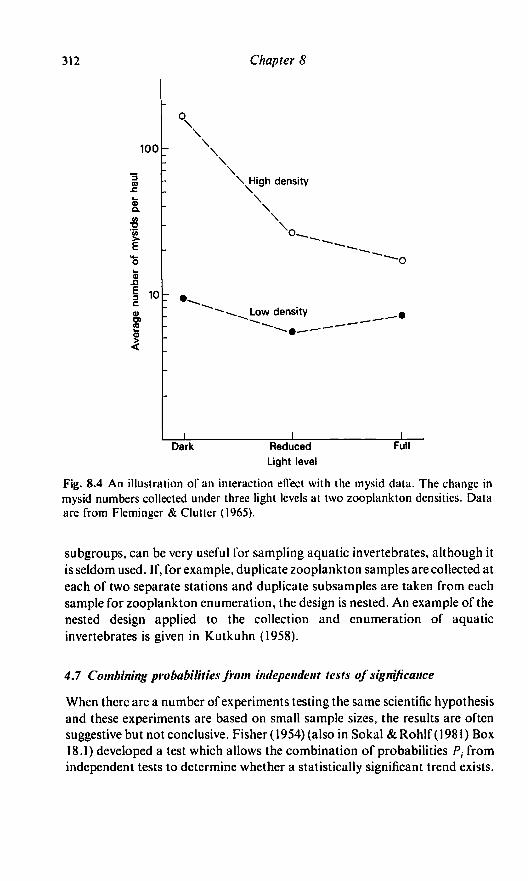
312 Chapter 8
100
2
10
\
\\\\\ High density
\\
Low density
**""—•—
Dark Reduced
Light level
Full
Fig. 8.4 An illustration of an interaction effect with the mysid data. The change in
mysid numbers collected under three light levels at two zooplankton densities. Data
are from Fleminger & Clulter (1965).
subgroups, can be very useful for sampling aquatic invertebrates, although it
is seldom used. If, for example, duplicate zooplankton samples are collected at
each of two separate stations and duplicate subsamples are taken from each
sample for zooplankton enumeration, the design is nested. An example of the
nested design applied to the collection and enumeration of aquatic
invertebrates is given in Kutkuhn (1958).
4.7 Combining probabilities from independent tests of significance
When there are a number of experiments testing the same scientific hypothesis
and these experiments are based on small sample sizes, the results are often
suggestive but not conclusive. Fisher (1954) (also in Sokal &Rohlf(1981) Box
18.1) developed a test which allows the combination of probabilities P, from
independent tests to determine whether a statistically significant trend exists.

Design of Experiments and Analysis of Samples 313
The natural logarithm (logc = In) is determined for each probability value Pt
and the statistic:
-2j>/>, (8-39)i= 1
is calculated where k is the number of independent tests and is distributed as a
y1 with 2k degrees of freedom.
This test is illustrated with results from four independent feeding trials
where the predator Neomysis was offered a choice between two groups of prey.
Daphnia sp. and Diaptomus ashkmdi (from Murtaugh 1981). For each
experiment the clearance rates (liters per predator per day) were compared
with a nonparametric equivalent to the /-test, the Wilcoxon rank sum test. The
Table 8.22 Results of feeding experiments where Neomysis were offered a choice
between Daphnia and Diaptomus. Probability values, Pj( are from a one-tailed
Wilcoxon rank sum test. Data are from Murtaugh (1981).
Experiment
(no. mysids)
1
(",=6)
2
("2 = 4)
3
in 3 = 7>
4
<«4=9)
Total
Prey
Daphnia
Diaptomus
Daphnia
Diaptomus
Daphnia
Diaptomus
Daphnia
Diaptomus
-2
Median clearance rate
(L mysid"1 day"1)
2-31
0-62
1-22
0-64
0-93
0-53
0-87
0-35
4
y ln/>;= -2(-9-50603) =191 = 1
Pi
0-021
0-243
0-180
0081
•01
\nP,
-3-863 23
-1-41469
-1-71480
-2-51331
-9-50603
significance probability levels for each experiment are given in Table 8.22.
Only one of the four tests was significant at the 95% confidence level.
However, when the probabilities are combined as illustrated in Table 8.22, the
resulting value is 19-01 and is compared with a ^-distribution with 8 degrees
of freedom. This result has a significance probability level between 0025 and
001. Therefore, the null hypothesis that Neomysis has no food preference
when offered a choice of Daphnia and Diaptomus ashlandi is rejected.

314 Chapter 8
5 Regression and Correlation
The analyses that have been considered so far involve single measurements on
each subject. However, the investigator is often interested in the dependence of
one variable on a second variable. This functional relationship is called
regression. Regression has many uses in biology, e.g., to describe the
relationship between water temperature and growth rate of an invertebrate.
The constants estimated in linear regression can be tested to determine
whether they are statistically different from zero or from any other number
chosen apriori. These constants can also be compared with those derived from
other populations. Finally, the linear regression model can be used for
prediction of one variable from another variable. If there is more than one
independent factor acting on the independent variable, a multiple regression
may be suitable.
The correlation coefficient is another measure of the relationship between
two variables. In correlation analysis there is no implied causal relationship of
one variable on the other, rather the interest is in the closeness of the
relationship. The correlation coefficient can be tested for significance, and, if
the sample size is sufficiently large, it can be used to describe the fraction of the
variability which can be explained by regression. However, correlation is more
limited than regression analysis because it cannot be used for making
predictions.
In this section the standard linear regression model is introduced and
compared with alternative models, the correlation coefficient is illustrated,
and more complex regression techniques are dealt with very briefly. The reader
is encouraged to consult textbooks which specialize in regression analysis
(e.g., Snedecor & Cochran 1980; Draper & Smith 1966) for a more extensive
account of these techniques.
5./ Standard linear regression
This is a parametric technique often referred to as Model I regression (Sokal &
Rohlf 1981). The estimation procedure used in standard linear regression is
that of least squares, and minimizes the squared deviations between each pair
of observed and predicted points. The linear model for a sample is:
Y=a+bX (8.40)
where A'and Fare the independent and dependent variables, respectively, and
a and b are the regression coefficients.
To develop a regression model, the independent and dependent variables
are defined. The independent variables should be under the control of the
investigator and be measured with relatively little error, whereas the
dependent variable varies freely. The independent variable should, ideally, be

Design of Experiments and Analysis of Samples 315
evenly spaced throughout its range. Notions ofcause and effect are implicit in
the choice of the variables.
In laboratory situations, the independent variable can be controlled but
this is often difficult or impossible in field situations. There are alternative
regression models which do not make assumptions about investigator control
of the independent variable. These approaches, referred to as Model II
regressions, are however, generally less powerful and the mathematics on
which they are based are poorly understood relative to the standard model.
Two of these alternative regression methods are discussed in a subsequent
section.
In standard linear regression, three assumptions are made about the
relationship between Y and X.
(1) If several Ys are chosen randomly for each A\ these Ys are normally
distributed.
(2) The population of Ys chosen for each X has a mean
fir = a + fiX (8.40i)
where a and fi are constants, i.e., fiy for different values of X lie on a
straight line.
(3) The variances about the mean nY are assumed to be homogeneous, i.e.,
the scatter around a mean regression line is similar over the entire range
of X.
In many cases, these assumptions cannot be tested and are assumed.
However, abnormal heterogeneity in the variances can be detected by
graphical means. This technique will be illustrated in the next section.
5.7.7 Preparation of data for analysis
Graphical techniques are useful for determining whether data are suitable for
linear regression. The independent variable is always placed on the horizontal
axis of a two-dimensional graph and the dependent variable on the vertical
axis. This technique is illustrated in Figs. 8.5 and 8.6 with data from
McCauley & Kalff (1981) (raw data supplied by E. McCauley) on the
phytoplankton-zooplankton relationship measured on individual dates in 13
lakes (Fig. 8.5a) and the average values for 17 lakes (Fig. 8.6a). The
phytoplankton-zooplankton relationship appears to be linear in both cases;
however, neither set of raw data is suitable for standard linear regression
analysis. In Fig. 8.5a the variance increases as the phytoplankton biomass
increases, and in both Figs. 8.5a & 8.6a the independent variables are not
evenly spaced; in Fig. 8.6a there is one extreme outlier and in Fig. 8.5a the
data become progressively thinner as the phytoplankton biomass increases.

250,000r
200,000
o>
150,000
o
J5c
5 100,000c
50,000
(a)
50,000 100,000 150,000
Phytoplankton biomass <mg m~3)
*r 5.00
4.00
3.00
2.00
0
(b)
3.00 4.00 5.00
Log phytoplankton biomass (mg m~3)
Fig. 8.5 Plots of zooplankton biomass against phytoplankton biomass based on
(a) indvidual observations from 13 lakes and (b) logI0 individual observations
from 13 lakes. Data are from McCauley & KahT(l981; E.McCauley, personal
communication).

Design of Experiments and Analysis of Samples
50,000 p
317
£ 40,000CO
30,000
| 20,000a
§N
0
jo 10,000
I
(a)
10,000 20,000 30,000 40,000 50,000
Average phytoplankton biomass (mg m~3)
6.0
5.0S3RJ
O
15
o
c 4.0(0
o
3.0
- (b)
0 3.0 4.0 5.0 6.0
Average log phytoplankton biomass {mg m~3)
Fig. 8.6 Plots of zooplankton biomass against phytoplankton biomass based on
(a) average observations from 17 lakes and (b) logI0 average observations from 17
lakes. Data are from McCauley & KalfT (1981; E.McCauley, personal
communication).
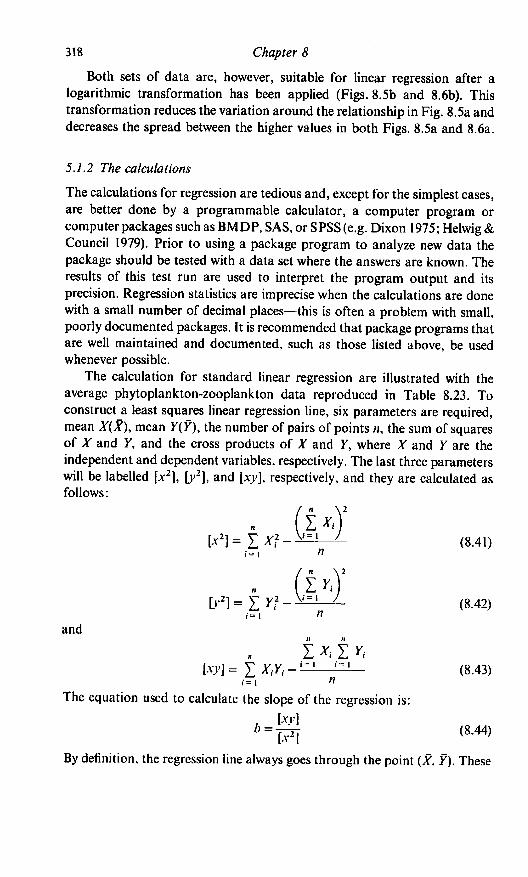
318 Chapter 8
Both sets of data are, however, suitable for linear regression after a
logarithmic transformation has been applied (Figs. 8.5b and 8.6b). This
transformation reduces the variation around the relationship in Fig. 8.5a and
decreases the spread between the higher values in both Figs. 8.5a and 8.6a.
5.1.2 The calculations
The calculations for regression are tedious and, except for the simplest cases,
are better done by a programmable calculator, a computer program or
computer packages such as BMDP, SAS, or SPSS (e.g. Dixon 1975; Helwig &
Council 1979). Prior to using a package program to analyze new data the
package should be tested with a data set where the answers are known. The
results of this test run are used to interpret the program output and its
precision. Regression statistics are imprecise when the calculations are done
with a small number of decimal places—this is often a problem with small,
poorly documented packages. It is recommended that package programs that
are well maintained and documented, such as those listed above, be used
whenever possible.
The calculation for standard linear regression are illustrated with the
average phytoplankton-zooplankton data reproduced in Table 8.23. To
construct a least squares linear regression line, six parameters are required,
mean X{X\ mean Y(Y), the number of pairs of points «, the sum of squares
of X and Y, and the cross products of X and 7, where X and Y are the
independent and dependent variables, respectively. The last three parameters
will be labelled [*2], [>>2], and [xy], respectively, and they are calculated as
follows:
I*.' (8-41)
1=1 n
^- (8.42)
andn n
[xy] = £ XtY, -i=l l = 1 (8.43),= , n
The equation used to calculate the slope of the regression is:
*-$By definition, the regression line always goes through the point (X, Y). These

Design of Experiments and Analysis of Samples 319
Table 8.23 Average phytoplankton and zooplankton biomass (mgm"J) expressed
as logj0 for 17 lakes. Data are from McCauley & Kalff (1981; E.McCauley, pers.
comra.).
Measured
Predicted
phytoplankton zooplankton zooplankton residual residual2
biomass biomass biomass (Yi - Y:) (Yt - f,)2
Xi Ys Ys
Total
mean
standard
deviation
s
2-631
2-651
2-708
2-756
3000
3017
3.086
3-125
3-234
3-322
3-612
3-643
3-825
3-950
4-037
4122
4-715
57-436
3-378 56
0-601 94
2-912
2-575
2-997
3-489
2-871
3131
3-833
3-310
3187
3103
3-469
3-504
3-745
4004
3-743
3-929
4-620
58-421
3-43655
0-508 25
2-893
2-907
2-949
2-984
3-161
3-174
3-224
3-252
3-331
3-395
3-606
3-629
3-761
3-852
3-915
3-977
4-408
001863
-0-3325
0-047 84
0-5047
-0-2904
-004304
0-609 3
0058 31
-01446
-0-2927
-01376
-0-1246
-001643
01516
-0-1722
-004856
0-2122
0
000035
011056
000229
0-25472
008433
0001 85
0-371 25
000340
002091
0-085 67
0-018 93
0-015 53
000027
0-02298
002965
000236
004503
107008
values are substituted into the regression equation (equation 8.40) along with
the value calculated for b to obtain the intercept:
a = Y-bX (8.45)
The variance about a regression line, called the residual variation, tr^., is
estimated from the sum of squared deviations of each observed value Y-t from
the corresponding predicted value Y,, = a + bXh divided by the degrees of
freedom for the regression line:
(8.46)v2 =±t=-''y.vn-2
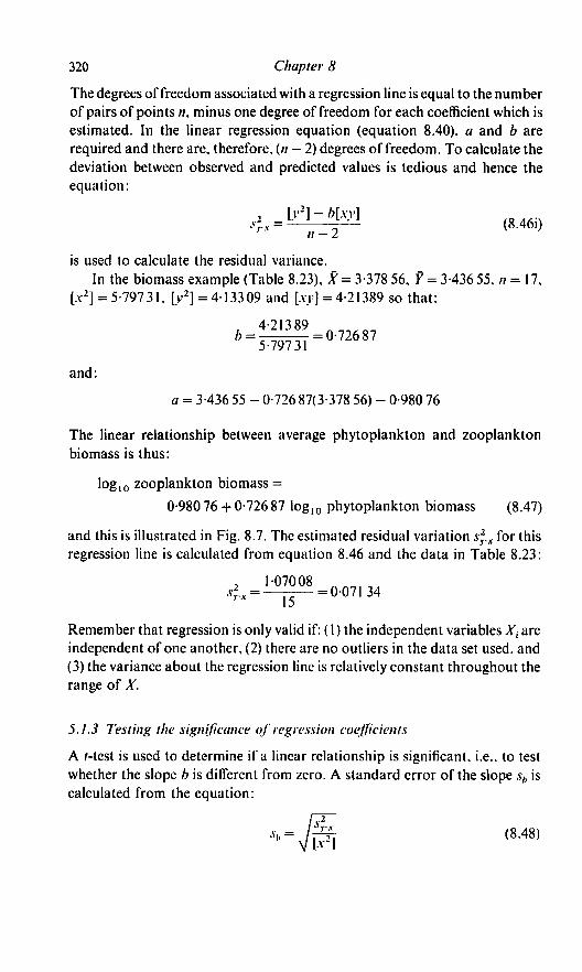
320 Chapter 8
The degrees offreedom associated with a regression line is equal to the number
of pairs of points «, minus one degree of freedom for each coefficient which is
estimated. In the linear regression equation (equation 8.40), a and b are
required and there are, therefore, {n - 2) degrees of freedom. To calculate the
deviation between observed and predicted values is tedious and hence the
equation:
i Iv2]-b[xy]
n-2(8.46i)
is used to calculate the residual variance.
In the biomass example (Table 8.23), * = 3-378 56, Y = 3-436 55. n = 17,
[x2] = 5-79731, [v2] = 4-13309 and [at] = 4-21389 so that:
and:
a = 3-436 55 - 0-726 87(3-378 56) - 0-980 76
The linear relationship between average phytoplankton and zooplankton
biomass is thus:
logi0 zooplankton biomass =
0-980 76 + 0-726 87 log10 phytoplankton biomass (8.47)
and this is illustrated in Fig. 8.7. The estimated residual variation sf..x for this
regression line is calculated from equation 8.46 and the data in Table 8.23:
,,,007,34
Remember that regression is only valid if: (1) the independent variables X-, are
independent of one another, (2) there are no outliers in the data set used, and
(3) the variance about the regression line is relatively constant throughout the
range of X.
5.1.3 Testing the significance of regression coefficients
A /-test is used to determine if a linear relationship is significant, i.e., to test
whether the slope b is different from zero. A standard error of the slope sb is
calculated from the equation:
■**= /ttff (8-48)

Design of Experiments and Analysis of Samples 321
5.0
4.0
| 3.0oo
2.0
3.0 4.0 5.0
Log average phytoplankton biomass (mg m~3)
Fig. 8.7 Regression of average zooplankton biomass on average phytoplankton
biomass. The narrower set of confidence bands is for the predicted value of the
mean /*, at point X and the wider set is for the predicted value of Y for a new
member of the population. Data are from McCauley & KalflT (1981; E.McCauley,
personal communication).
where s]..x is the residual variation and [.v2] the sum of squares of X. The ratio:
/ =
b-0(8.48i)
is compared with a Student's /-distribution with {n - 2) degrees of freedom. In
the biomass example:
= 0110 93
and:
0-72687 ^cc
' = (HT093 =6'55
This / value is compared with a Student's /-distribution with 15 degrees of
freedom. Since the significance probability is <0-0001, the null hypothesis
that the slope of the regression line is not difierent from zero is rejected.
Confidence intervals for the slope are calculated from the relationship:
b±sbt (8.48ii)
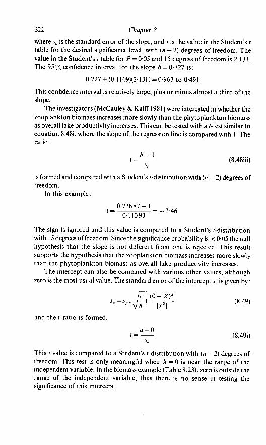
322 Chapter 8
where sb is the standard error of the slope, and / is the value in the Student's t
table for the desired significance level, with (n - 2) degrees of freedom. The
value in the Student's t table for P = 005 and 15 degress of freedom is 2-131.
The 95% confidence interval for the slope h = 0-727 is:
0-727 ±(0-1 IO9)(2-131) = 0-963 to 0-491
This confidence interval is relatively large, plus or minus almost a third of the
slope.
The investigators (McCauley & KalfiT 1981) were interested in whether the
zooplankton biomass increases more slowly than the phytoplankton biomass
as overall lake productivity increases. This can be tested with a /-test similar to
equation 8.48i, where the slope of the regression line is compared with 1. The
ratio:
b-\t = (
is formed and compared with a Student's r-distribution with (n - 2) degrees of
freedom.
In this example:
0-72687-1
246" 01.093 246
The sign is ignored and this value is compared to a Student's /-distribution
with 15 degrees of freedom. Since the significance probability is <0-05 the null
hypothesis that the slope is not different from one is rejected. This result
supports the hypothesis that the zooplankton biomass increases more slowly
than the phytoplankton biomass as overall lake productivity increases.
The intercept can also be compared with various other values, although
zero is the most usual value. The standard error of the intercept sa is given by:
(0 - xy
—TJT- (8-49)
and the /-ratio is formed,
_a-0(8.49i)
This / value is compared to a Student's /-distribution with (n - 2) degrees of
freedom. This test is only meaningful when X = 0 is near the range of the
independent variable. In the biomass example (Table 8.23), zero is outside the
range of the independent variable, thus there is no sense in testing the
significance of this intercept.

Design of Experiments and Analysis of Samples 323
5.1.4 Confidence intervals about predicted values
There are different confidence intervals for two types of predicted values. To
calculate the confidence interval for the mean n? = ol + pX at point Xh a
standard error of the predicted value s(n?) is required:
I (X; ~ X)2
» [-v2] (8-50)where syx is the square root of the residual variation, n is the number of pairs
of points, [a:2] is the sum of squares of X, and X is the mean of the independent
values. The 95% confidence interval is calculated from the formula:
l*t±s(nt)t (8.50i)
where / is the value in the Student's t table with (n — 2) degrees of freedom and
probability level 005.
For example, for a phytoplankton biomass (logI0) of 3-950mgm"3 the
predicted mean zooplankton biomass (log,0) is 3-852mgm"3 (Table 8.23).
The standard error of this predicted value fiy = 3-852 mgm"3 is:
and the 95% confidence interval is:
3-852 ±00906(2-131) =4045 to 2040 mg m"3
as illustrated in Fig. 8.7. The size of the confidence interval increases with the
distance between X( and X: when the measured phytoplankton biomass is
4-715mgm"3, the predicted mean zooplankton biomass is 4.408mgm"3.
The standard error of fif = 4-408 is:
and the confidence interval is ±0-3448 as compared to ±01931 mgm"3 in
the previous example.
A regression equation can also be used to predict the value of Y for an
individual that was not used to construct the regression line. The predicted
value Y is calculated from the standard equation Y = a + bX\ there is,
however, greater uncertainty associated with the prediction of Y than the
mean [if, which is reflected in a larger error term. The equation used to
calculate this standard error .v, is:
(8.SD

324 Chapter 8
The value of Sy also increases as the distance between the measured value X{
and the mean X increases. The formula for the 95 % confidence interval is
Y±Sft (8.5 li)
where / is the value in the Student's / table with (/? — 2) degrees of freedom and
probability level 005.
For example, the standard errors of the predicted (log]O) zooplankton
biomass of 3-852 and 4-408 mgm ~3 for new individual lakes with measured
(log,0) phytoplankton biomass of 3-950 and 4-715mgm"3 are
and
respectively. The 95% confidence limits for Y = 3-852 are ±0-6009mgm"3
and for Y = 4-408 they are ±0-6655 mg m 3. These are much larger than the
confidence intervals for the mean zooplankton biomass at the same A>, as
illustrated in Fig. 8.7.
If predictions are made for several new members of the population, the
confidence interval for each of the new members is larger than the confidence
interval obtained if there was only one new member. For example, if
confidence intervals are constructed from equation 8.5li for each of 12 new
lakes, the probability that all 12 confidence intervals include the correct values
of the new Ks is substantially less than 0-95. The method for calculating
confidence intervals for several values of Y is detailed in Snedecor and
Cochran (1980. p. 166).
Since the relationship for individuals outside the range of the values in the
original data set is unknown, predictions should not be attempted for such
individuals. Thus, equation 8.47 should not be used to make predictions when
the average phytoplankton biomass is < 2-631 or >4-715 (log,0)mgm~3.
5.2 Alternatives to standard linear regression
Standard linear regression makes certain assumptions which arc often not
satisfied by biological data, particularly those which are collected in the field.
For example, the independent variable should either be measured without
error or be under investigator control. However, the phytoplankton data
(Table 8.23) do not satisfy this assumption. In such circumstances the
investigator may turn to alternative models which make fewer assumptions.
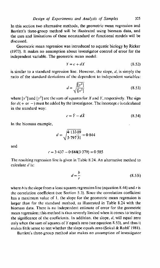
Design of Experiments and Analysis of Samples 325
In this section two alternative methods, the geometric mean regression and
Bartlett's three-group method will be illustrated using biomass data, and
the uses and limitations of these nonstandard or functional models will be
discussed.
Geometric mean regression was introduced to aquatic biology by Ricker
(1973). It makes no assumption about investigator control of error for the
independent variable. The geometric mean model:
Y = c + dX (8.52)
is similar to a standard regression line. However, the slope, d, is simply the
ratio of the standard deviations of the dependent to independent variables:
<8-53)where [,v2] and [y2] are the sum of squares for A'and Y, respectively. The sign
for d( + or -) must be added by the investigator. The intercept c is calculated
in the standard way:
c = Y-dX (8.54)
In the biomass example,
/413309 nd= / = 0-844
V5-79731
and
c = 3-437 - 0-844(3-379) = 0-585
The resulting regression line is given in Table 8.24. An alternative method to
calculate d is:
d = - (8.53i)r
where b is the slope from a least squares regression line (equation 8.44) and r is
the correlation coefficient (see Section 5.3). Since the correlation coefficient
has a maximum value of 1. the slope for the geometric mean regression is
larger than for the standard method, as illustrated in Table 8.24 with the
biomass data. There is no independent estimate of error for the geometric
mean regression: this method is thus severely limited when it comes to testing
the significance of the coefficients. In addition, the slope, d, will equal zero
only when the sum of squares of Y equals zero (see equation 8.53), and thus it
makes little sense to test whether the slope equals zero (Sokal & Rohlf 1981).
Bartlett's three-group method also makes no assumption of investigator

326 Chapter 8
Table 8.24 Regression lines fit to the phytoplankton (A'), zooplankton (Y) biomass
data (mg m"3) in Table 8.23. Data are from McCauley & KahT(1981;
E.McCauley, pres. comm.).
Standard linear regression
log10}'= 0-981+0-727 logj0A-
Geometric mean regression
log10y = 0-585 + 0-844 log,0Jf
Bartlett's three-group method
log10r = 0-938 +0-739 log,0A-
control oferror in the independent variable. The regression has the same form
as the previous models:
Y = e+JX (8.55)
To estimate the regression coefficient./, the data are arranged in ascending
order with respect to X, as in Table 8.23. Then they are divided into three
groups of approximately equal size. The first and last group must be of equal
size, as illustrated in Table 8.25. Mean X and Y values are calculated for
groups one (Xlt Y,) and three (X3, f3), in order to calculate the regression
coefficients:
/■ F3 - YiJ =^—F (8.56)
and:
e = Y-j~X (8.57)
In the biomass example:
r 3-924-2-996
^4-049-2-794 = °-739e = 3-437 - 0-739 44(3-379) = 0-938
and the regression line is given in Table 8.24. Confidence intervals for this
method involve several additional calculations, as illustrated in Sokal & Rohlf(1981, Box 14.12).
The two functional regression lines for the biomass data are different from
each other and from the least squares equation (see Table 8.24), and,
therefore, the question of which regression line should be used arises.
Unfortunately, the mathematical basis of functional regression is not
sufficiently well worked out to answer this question. There are other
weaknesses with both functional regression methods outlined here (e.g.,
Ricker 1973; Kuhry & Marcus 1977). For example, it is still uncertain what
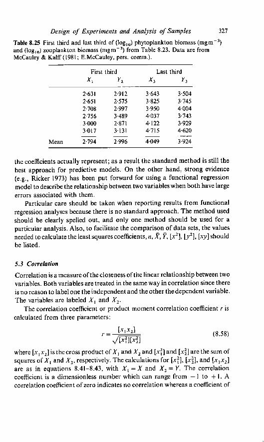
Design of Experiments and Analysis of Samples 327
Table 8.25 First third and last third of (log10) phytoplankton biomass (ragm"3)
and (log10) zooplankton biomass (mgm~3) from Table 8.23. Data are from
McCauley & Kalff (1981; E.McCauley, pers. comm.).
First third Last third
2-631
2-651
2-708
2-756
3000
3-017
2-912
2-575
2-997
3489
2-871
3131
3-643
3-825
3-950
4-037
4-122
4-715
3-504
3-745
4004
3-743
3-929
4-620
Mean 2-794 2-996 4-049 3-924
the coefficients actually represent; as a result the standard method is still the
best approach for predictive models. On the other hand, strong evidence
(e.g., Ricker 1973) has been put forward for using a functional regression
model to describe the relationship between two variables when both have large
errors associated with them.
Particular care should be taken when reporting results from functional
regression analyses because there is no standard approach. The method used
should be clearly spelled out, and only one method should be used for a
particular analysis. Also, to facilitate the comparison of data sets, the values
needed to calculate the least squares coefficients, n, X, Y, [x2], [y2], [xy] should
be listed.
5.3 Correlation
Correlation is a measure of the closeness ofthe linear relationship between two
variables. Both variables are treated in the same way in correlation since there
is no reason to label one the independent and the other the dependent variable.
The variables are labeled X{ and X2.
The correlation coefficient or product moment correlation coefficient r is
calculated from three parameters:
(8.58)
where [x,.y2] is the cross product of A', and X2 and [xj] and [xj] are the sum of
squares of A', and X2, respectively. The calculations for [x2], [xj], and [x,jc2]
are as in equations 8.41-8.43, with Xx = X and X2 = Y. The correlation
coefficient is a dimensionless number which can range from — 1 to 4-1. A
correlation coefficient of zero indicates no correlation whereas a coefficient of

328 Chapter 8
Table 8.26 Total phosphorus loading (Lp, gm 2yr l) and number of crustaceans
(cm"2) in four Great Lakes. Data are from Patalas (1972).
Lake Crustaceans
X,
XXX1 X] Rank
1849
27 889
93636
160000
Lp
1
2
3
4
Crustaceans
1
2
3
4
Superior
Huron
Ontario
Erie
0-03
0-15
0-86
0-98
43
167
306
400
Total 2-02
1 -29 00009
25-05 0-0225
263-16 0-7396
392-00 0-9604
916 681-50 1-7234 283 374
=218-92
[.v2] = 1 -7234 - = 0-7033
[.v2] = 283 374 -<^- = 73 610
218-92= 0-96
7033X73 610)
1 indicates that the correlation is perfect. The calculations for a correlation
coefficient are illustrated in Table 8.26 with data from Patalas (1972) on the
levels of phosphorus loading and crustacean numbers in four Great Lakes.
Correlation has two frequent uses. In regression it describes the
proportion of the variation in Y that can be attributed to its linear regression
on X. It is also used to determine whether the correlation between two
variables is significantly different from zero. This latter requires that the points
are independent and follow a bivariate normal distribution. A bivariate
normal distribution is a cloud of points in an elliptical band, similar to those in
Fig. 8.5b.
The square of the correlation coefficient, r2, is the fraction of the variance
of X2 that can be attributed to its linear regression on Xx when the sample
size is large. Although an r2 value could be calculated for the crustacean
biomass example, a sample size of four is too small for the results to be
meaningful. On the other hand, an r2 value can be interpreted for the logged
individual phytoplankton-zooplankton biomass data, illustrated in Fig. 8.5b.
Since [x2] = 106-32, [x22] = 72-66, and [xlx2] = 53-48 for this example, the
correlation coefficient is:
;=0-61

Design of Experiments and Analysis of Samples 329
and
/■2 = 0-37
Thus, 37% of the variance of the zooplankton data in Fig. 8.5b can be
attributed to its linear regression on phytoplankton biomass.
To test if the correlation coefficient is significantly different from zero, it is
compared to the critical values for correlation coefficients with (n - 2) degrees
of freedom. The crustacean biomass data in Table 8.26, with r = 0-96 and a
sample size n = 4 will be used as an illustration. For 2 degrees of freedom, the
5 % value of r in a table of critical values is 0-95. The observed r is statistically
significant and the null hypothesis that there is no correlation between
phosphorus loading and crustacean biomass in the Great Lakes is rejected.
The crustacean biomass example is not entirely suitable for testing the
significance of the product moment correlation coefficient because a sample
size of four is too small to know whether either of the variables was from a
normally distributed population. Some tables for the critical values do not
even cover 2 degrees of freedom (e.g., Snedecor & Cochran 1980). The
nonparametric alternative to the product moment correlation coefficient is the
Spearman rank correlation coefficient. This is used when neither variable
follows the normal distribution; it is less powerful than the parametric
equivalent for small samples and quite tedious to perform for large samples. In
this procedure. Xx and X2 are both converted to rankings as illustrated with
the crustacean biomass data in Table 8.27. The difference between the ranks
for each pair of points, <7,, is used to calculate the rank correlation coefficient:
6 yi =
{ , (8.59)/?(/r — 1)
where there are n pairs of points. In the crustacean biomass example, rs = 1,
suggesting a strong correlation. However, there is no critical value at the 95 %
confidence level for a Spearman rank correlation coefficient when the sample
Table 8.27 The ranks of the paired variables; total phosphorus loading (Lp) and
number of crustaceans in four Great Lakes from Table 8.26. Data are from
Patalas (1972).
Lake
Superior
Huron
Ontario
Erie
Lp
1
2
3
4
Rank
Crustaceans
1
2
3
4
Difference
0
0
0
0

330 Chapter 8
size is 4. Thus, the null hypothesis that phosphorus loading and crustacean
biomass are not correlated in the Great Lakes cannot be rejected with this test.
In order to illustrate the limitations of nonstandard correlation and
regression tests, the same examples were used for more than one test. In
practice, data should be analyzed by only one method, chosen prior to the
analysis. This is because a variety of analyses may give more than one result
and the decision of the investigator to choose one method over the others may
be based on the results. As illustrated, crustacean numbers and phosphorus
loading in the Great Lakes are significantly correlated at the 95 % confidence
level with a standard correlation but not with a rank correlation. The choice of
method will obviously influence the result in this case.
Correlation is most meaningful when it is carried out on data selected to
test a specific hypothesis. When data are available on several parameters it is
often tempting to run correlations on all possible sets of parameters. However,
when a shotgun approach is used, the probability of erroneously reporting
significant results increases, i.e., if you look at data in enough ways, patterns
will be found even if the data are generated randomly (e.g., Cole 1954, 1957).
5.4 Some other regression models
In this section other models in regression—multiple linear, polynomial, and
nonlinear—and the comparison of regression lines or analysis of covariance
are mentioned. These are complex subjects and users are encouraged to
consult texts such as Draper & Smith (1966) and Snedecor & Cochran (1980)
for an introduction to them.
5.4.1 Multiple linear regression
Multiple linear regression is the linking of two or more independent variables
to a single dependent variable. When there are two independent variables Xx
and X2 the multiple linear regression equation for a sample is:
Y = a + bxXx+b2X2 (8.60)
where a, bx. and b2 are sample coefficients, and Y is the predicted value. The
coefficients bx and b2 can be tested for significance to determine if a multiple
regression is more suitable than a linear regression.
For example. Grant & Bayly (1981) used both a measure of turbulence and
the density of an invertebrate predator Anisops to predict variation in crest
size in Daphnia cephalata. The measure of turbulence accounted for 78 % of
the variation in crest size in a linear regression, whereas when the measure of
turbulence was combined with density of predators in a multiple regression,
they accounted for 88 % of the variation in crest size. In this case, a multiple

Design of Experiments and Analysis of Samples 331
regression explained significantly more of the variation than the simple
regression.
Multiple linear regression, like many other complex models in regression,
requires a much larger sample size than simple regression. The variables Xx
and X2 should be independent ofeach other, so that appropriate values can be
assigned to the coefficients bx and b2.
5.4.2 Nonlinear regression
The relationship between two variables is often not a straight line. If the
population size is sufficiently large a polynomial regression of the form:
2X2 + --- + b,,X" (8.61)
can describe the relationship between two variables X and Y, where a, b{,
b2 bn are coefficients, and n is the order of the polynomial.
For example, based on laboratory results, Frank el al. (1957) described the
relationship between age and volume of Daphnia pulex with the polynomial
equation:
X = 01928 +0-327*-6-514-KT3*2* 51 5691(T5A'3
where X is age in days and Y is number cm " 3. For these data a third degree
polynomial described 99 % of the variance.
Many other nonlinear regression models are available, e.g., the exponential
growth model:
Y = (a)(bx) (8.62)
and the exponential decay model:
Y = (a)(b~x) (8.63)
where A'and Y are the independent and dependent variables, respectively, and
a and b are the coefficients. The exponential growth model is commonly used
to describe the change in weight of young organisms (Y) over time (X). The
exponential decay model can be used to describe development time (Y) of
immature stages of aquatic organisms at various temperatures.
The coefficients in regression models should always be tested for
significance. If several parametric models seem appropriate, the one which has
significant coefficients and accounts for the highest fraction of the variation
should be used.
5.4.3 Analysis of covariance
The relationship between two or more variables can be compared for various
treatments with an analysis ofcovariance. For example, Cooley (1977) used an
332 Chapter 8
analysis of covariance to examine the effect of pulp mill effluent on filtering
rates ofDaphnia retrocurva. He measured the filtering rates (ml per animal per
day) and carapace lengths (mm) of Daphnia in lake water (with labeled algae
added) with and without pulp mill effluent. Filtering rate was regressed on
body size for each treatment and the regression lines were compared. These
results could have been analyzed by an analysis of variance if animals of
identical size were used in both treatments. However, as this is virtually
impossible with Daphnia, and since body size has an important influence on
filtering rate, an analysis of covariance is the appropriate analytical method.
Analysis of covariance should only be used when the covariates (such as body
size) are drawn from the same population.
Comparison of regression lines in analysis of covariance is done in three
parts. First, the residual variances of the individual regression lines are
compared. If these variances are homogeneous, a common residual variance is
calculated and the individual slopes are compared. If these slopes are not
significantly different, a common slope is calculated along with an adjusted
common residual variance and the individual adjusted intercepts are
compared. When more than two regression lines are compared, the methods
outlined for multiple comparisons of means (Section 4.5) are applied.
6 Summary
The trend in data analysis is towards more sophisticated techniques. However,
as the complexity of the analysis grows, there is a tendency to lose sight of the
original biological questions and the analysis tends to take on a meaning
independent of the original intention of the investigation. I am reminded at
this point of a paper which appeared recently in a major journal. Multivariate
analyses were applied to a large data set and the results were spelled out in
great detail, yet there was no mention of the variables used in the analysis, let
alone how they were determined.
The contribution of any analysis is dependent upon three factors; the
experimental design, the quality of the data, and the suitability of the method
of analysis for the data. Weakness in any one of these areas can override any
significant results. When writing up an experiment, one should present
sufficient information so that the results are clearly understood and
demonstrated by the data. In summary:
(1) The data should be collected with specific analysis in mind.
(2) The samples should be of sufficient size for the analyses.
(3) The data should be examined carefully for suitability for the selected
analyses.

Design of Experiments and Analysis of Samples 333
(4) The raw data should be presented or at least a summary should be given
(e.g., mean, standard deviation, and sample size).
(5) The results of the analyses should be clearly spelled out and related to the
scientific questions asked.
7 References
Box G.E.P. & Cox D.R. (1964) An analysis of transformation. J. Roy. Stat. Soc, Ser.
B, 26, 211-243.
Cassie R.M. (1963) Tests of significance for probability paper analysis. N.Z. J. Sci., 6,
474-482.
Cochran W.G. (1954) Some methods for strengthening the common %2 tests.
Biometrics, 10,417-451.
Cochran W.G. (1977) Sampling Techniques. New York: Wiley.
Cole L.C.( 1954) Some features of random population cycles. J. Wildlife Management
18, 2-24.
Cole L.C. (1957) Biological clock in the unicorn. Science, 125, 874-876.
Conover W.J. (1980) Practical NonparametricStatistics. (2nd ed.) New York: Wiley.
Cooley J.M. (1977) Filtering rate performance of Daphnia retrocurva in pulp mill
effluent. /. Fish. Res. Board Can., 34, 863-868.
David H.A. (1952) Upper 5 and I % points of the maximum F-ratio. Biometrika 39422-424.
Dixon W.J. (1975) BMDP. Biomedical computer programs. Berkeley: University of
California Press.
Downing J.A. (1979) Aggregation, transformation, and the design of benthos
sampling programs. J. Fish. Res. Board Can., 36, 1454-1463.
Draper N. & Smith H. (1966) Applied Regression Analysis. New York: Wiley.
Dunnett C.W. (1955) A multiple comparison procedure for comparing several
treatments with a control. J. Amer. Statistical Assoc, 50, 1096-1121.
Dunnett C.W. (1964) New tables for multiple comparisons with a control. Biometrics-20,482-491.
Edmondson W.T. (1960) Reproductive rates of rotifers in natural populations. Mem.1st. Ital. Idmbiol., 12, 21-77.
Elliott J.M. (1977) Some Methodsfor the Statistical Analysis of Samples of Benthic
Invertebrates. Scientific publ. No. 25 (2nd ed.) Freshwater Biol. Assoc.
Fisher R.A. (1954) Statistical Methodsfor Research Workers. (12th ed.) Edinburgh:
Oliver & Boyd.
Fleminger A. & Clutter R.I. (1965) Avoidance of towed nets by zooplankton. Limnol.
Oceanogr., 10, 96-104.
Frank P.W., Boll CD. & Kelly R.W. (1957) Vital statistics of laboratory cultures of
Daphnia pulex De Geer as related to density. Physiol. Zool., 4, 288-305.
Grant J.W.G. & Bayly I.A.E. (1981) Predator induction of crests in morphs of the
Daphnia carinata King complex. Limnol. Oceanogr., 26. 201-218.
Green R.H. (1979) Sampling design and statistical methods for environmentalbiologists. New York: Wiley.
Helwig J.T. & Council K.A. (1979) The SAS user's guide. Raleigh, North Carolina,
USA: SAS Institute, Inc.
334 Chapter 8
Iwao S. (1977) The m*-m statistic as a comprehensive method for analyzing spatial
patterns of biological populations and its application to sampling problems Jpn.
Int. Biol. Prog. Syn., 17, 21-46.
Keuls M. (1952) The use of 'studentized range' in connection with an analysis of
variance. Euphytica, 1, 112-122.
Kott P. (1953) Modified whirling apparatus for the subsampling of plankton. Aust. J.
Mar. Freshw. Res., 4, 387-393.
Kuhry B. & Marcus L.F. (1977) Bivariate linear models in biometry. Sysi. Zool., 26,
201-209.
Kutkuhn J.H. (1958) Notes on the precision of numerical and volumetric plankton
estimates from small-sample concentrates. Limnol. Oceanogr., 3, 69-83.
Lampert W. (1974) A method for determining food selection by zooplankton. Limnol.
Oceanogr., 19, 995-998.
Lloyd M. (1967) Mean crowding. J. Anim. EcoL, 36, 1-30.
May J.M. (1952) Extended and corrected tables of the upper percentage points of the
kstudentized' range. Biometrika, 39, 192-193.
McCauley E. & KalfT J. (1981) Empirical relationships between phytoplankton and
zooplankton biomass in lakes. Can. J. Fish. Aquat. 5c/., 38, 458-463.
Murtaugh P.A. (1981) Selective predation by Neomysismercedisin Lake Washington.
Limnol. Oceanogr., 26, 445-453.
Newman D. (1939) The distribution of range in samples from a normal population
expressed in terms of an independent estimate of standard deviation. Biometrika,
31, 20.
Patalas K. (1972) Crustacean plankton and the eutrophication of St. Lawrence Great
Lakes. J. Fish. Res. Board Can., 29, 1451-1462.
Peters R.H. & Rigler F.H. (1973) Phosphorus release by Daphnia. Limnol. Oceanogr.,
18, 821-839.
Pielou C.E. (1977) Mathematical Ecology. New York: Wiley.
Prepas E.E. & Trew D.O. (1983) Evaluation of the phosphorus-chlorophyll
relationship for lakes off the Precambrian Shield in western Canada. Can. J. Fish.
Aquat. Sci., 40. 27-35.
Ricker W.E. (1937) Statistical treatment of sampling processes useful in the
enumeration of plankton organisms. Arch. Hydrobiol., 31, 68-84.
Ricker W.E. (1938) On adequate quantitative sampling of pelagic net plankton of a
lake. J. Fish. Res. Board Can., 4, 19-32.
Ricker W.E. (1973) Linear regressions in fishery research. J. Fish. Res. Board Can., 30,
409-434.
Rigler F.H. & Langford R.R. (1967) Congeneric occurrences of species of Diaptomus
in southern Ontario lakes. Can. J. Zool., 45, 81-90.
Rohlf F.J. & Sokal R.R. (1981) Statistical Tables. San Francisco: Freeman.
Schefle H. (1959) The Analysis of Variance. New York: Wiley.
Siegel S. (1956) Nonparametric Statistics for the Behavioural Sciences. New York:
McGraw-Hill.
Snedecor G.W. & Cochran W.G. (1980) Statistical Methods. (7th ed.) Ames, Iowa:
State Univ. Press.
Sokal R.R. & Rohlf F.J. (1981) Biometry. San Francisco: Freeman.
Steel R.G.D. & Torrie J.H. (1960) Principles and Procedures ofStatistics. New York:
McGraw-Hill.
Design of Experiments and Analysis of Samples 335
Stuart A. (1962) Basic Ideas of Scientific Sampling. London: Latimer, Trend & Co.Taylor L.R. (1961) Aggregation, variance, and the mean. Nature, 189, 732-735.
Taylor L.R. (1980) Comment on 'Aggregation, transformation, and the design ofbenthos sampling programs.' Can. J. Fish. Aquat. Sci., 215-219.
Tukey J.W. (1949) One degree of freedom for non-additivity. Biometrics, 5,232-242.Tukey J.W. (1977) Exploratory Data Analysis. Reading, Massachusetts :Addison-
Wesley.
Zar J.H. (1974) Biostatistical Analysis. Englevvood Cliffs, N.J.: Prentice-Hall.

Chapter 9. Methods for the Study of Feeding,
Grazing and Assimilation by Zooplankton
ROBERT HENRY PETERS
1 Introduction
In terms of energy or mass flow, ingestion represents the greatest of all
interactions between an animal and its environment (Spomer 1973).
Consequently, many aquatic ecologists have attempted to describe and
measure the feeding process of zooplankton. They have evolved a formidable
number of methods.
Any investigation must be tailored to the hypotheses to be tested; it is,
therefore, important to consider briefly the major questions to which
zooplankton ingestion and assimilation are relevant. At a practical level, there
are two: we wish to know the future amount and composition of the algal
community and we wish to predict fish stocks. The former is determined, in
part, by the pressure of zooplanktonic grazing on the algae and the latter, in
part, by the amount of zooplankton production available to the fish. Of
course, accurate descriptions of the feeding process of zooplankton alone will
not permit predictions about fish stocks or algal composition: such
descriptions can only be used as components in larger models of the aquatic
ecosystem which will yield such predictions. At a more academic level,
zooplankton lend themselves to the testing of ecological theory because of the
animals' small size, ease of culture, aquatic habitat and the seemingly reduced
heterogeneity of their environment. Determinations of ingestion and grazing
rates have been used in studies dealing with energy flow (Slobodkin and
Richman 1956; Richman 1958), mineral cycling (Johannes 1968; Peters &
Rigler 1973), competition (Dodson 1970; Hall et al. 1976; Lynch 1977),
optimal foraging (Lam & Frost 1976; Lehman 1976), and predator-prey
interactions (Holling 1959; Wilson 1973) among others. Beyond these general
theories lie an unlimited number of specific hypotheses regarding the fine
structure of aquatic communities and the behavior of their components. This
review primarily presents the basic methods which have been used to measure
feeding, grazing and assimilation rates. I hope these methods will not be
adopted uncritically by other workers but will be adapted to suit their own
needs and their questions.
336


![AdvancedMeasuring(Instrumentation)Methodsfor ...steady-state sensor locations in international thermonuclear experimental reactor [2]. They used the tissue equivalent proportional](https://img.pdfslide.us/doc/110x75/6105e01ea3b1f254d87f5a0d/advancedmeasuringinstrumentationmethodsfor-steady-state-sensor-locations-in.jpg)