CHAPTER 8

WWT EmONENT APPLIED TO STUDY THE STOCICIASTIQ: NATURE OF VAL MEAN VALUES

Hurst exponent is an important measurement in fractal analysis, descriptions of rough

images and signals. The geomapetic annual mean values of the horizontal (H) component for

the five Indian geomagnetic observatories are analyzed in this chapter by eernpiioying the

technique of Hurst exponent.

8.1 Introduction

A self-affine set is statistically invariant under an affine transformation. A 2-dimensional

surface described by a h c t i o n f (x, y) is a self-&me fractal, if there exists a number W such that

f ( ~ , ~ ) = h - ~ f ( ~ J ~ Y ) (8- 1)

where h is a positive nuiber.

The number H in (8.1) is called the Hurst exponent or HausdorfT exponent or self-aEne

exponent. H takes a value between 0 and 1, that is 0 5 H 5 1 . [84].

For a background on Humt exponent, one may refer Mandelbrot [44], Turcottee [Sl],

Malamute [42] and Wanlis and Reynolds [82J.

The equation (8.1) indicates that f (Is, hHy) is statistically similar to f (x, y) with a

similarity exponent H. In one-dimension, a self-affine fractal is defined as

f (x) = f (Ax) (8.2)

In this case, x and f(x) are often interpreted as the time and the corresponding tr~jectory

(position), respectively. It has been proved that the Hurst exponent, H, and the self-affine fractal

dimension, or the box-counting dimension, D, are related by the equation

H = 2 - D (8.3)

Therefore the condition 1 5 D 5 2 corresponds to the relation 0 5 H I 1 for a self-&fine

*dctal. If H = 1, the self-&he hc ta l becomes self-similar, which is by definition isotropic. A

stochastic process or a surface with H > 1/2 is said to be persistent, and that with H < ?4 is said to

be anti persistent.

Following MaIamud and Turcottee [42], [43] and Turcottee [81], the basic property of a

self-affme time series is that the power spectral density of the time series has a power-law

dependence on fi-equency.

114

Wurst exponent KT has broad applications for studies on earth quakes, activities prior to

geomgneiic storms, to ensure the stochastic nature of geomagnetic variations, fractal metrology

for images, signals in time series analysis, geomagnetic activity of the Dst index, etc. Wurst

component can distinguish a random series from a nonrandom series. Measurement of Hust

exponent can be applied in the power spec tm analysis, wavelet trmsfoms, fractals and

measurement of stochastic nature in time series analysis. Hurst exponent has been studied for

various nonlinear processes in geophysics. UILF geomagnetic dzta of the most intense horizontal

H component observed at G m observatory has been analyzed by Ida et.al PO] by estimating

the generalized Hurst component and significant changes in the muEti fiactd parameters which

showed a decrease of about 25 days before earthquake. A degree of non-stationary of

geophysical medium can be evaluated by analyzing temporal variations of certain characteristics

of stdied signals. The Wurst exponent obtained from the analysis of temporal fluctuations in the

inter-event intervals of the earthquakes and exponent of the power spectrum, which behaves as a

power-law function of the fiequency was considered for earthquake prediction by Decherevsky

et.aI [21]. Measurement of Hurst exponent is an effective tool to study the ground magnetometer

measurement of total magnetic field strength, as reported by Wanliss and Reynolds [XZ]. This

technique has been employed in the analysis of geomagnetic activity of the Dst index by Wei and

Billings et.al [84]), pre-storm activity to geomagnetic storm by Balasis et-a1 [9] and fractal

metrology for images, signals and time series processing by Oleschko and Tarquis [52].

The analysis by Hurst is termed as 'Rescaled Analysis' or 'R / S Analysis'. Hurst [29]

found that most natural phenomena such as temperature, rain fall, sunspots, etc., follow a 'biased

random walk', i-e., a trend with noise. The strength of the trend and the level of noise could be

measured by how the rescaled ranges with time, that is by how high the exponent H is above

0.50. Long memory or long term dependency describes the correlation stnrctme of a series at

long lags. If a series exhibits long memory, there is persistent ternporal dependence, even

between distant observations. IvIandelbrot [46] characterized long memory processes as the one

having fractal dimension. Long memory time series were first suggested by Bernard [lo] as a

possible cause of the Hurst [29] effect. Bennard [lo] pointed out that auto covariance hc t ion of

such a long memory time series is not summable and several authors like Hipel and Meleod [27]

used this as the defrition of long memory. The most widely used test for fractal dimension and

long memory time series are the rescaled range (RIS) analysis introduced by Hurst [29] and later

refined by Mandelbrot E461- Anatyticai technique arnd the results of the analysis are explained in

this ckaprer.

8.2 Pessistel~t t h e series

Suppose a xime series has been up (down) in the last period. Suppose that the chances are

Glat it will continue to be positive (negative) in the next period. Then the series is said to be a

persisten? time series.

8 3 Ibmti persistent t h e series

Suppose a tirne series has been up in the previous period. Suppose that most likely it will

be down in the next period. Then the system is called an anti persistent tirne series.

8.4 Long memory

A time series (Xt) is said to be of long memory if its auto conelation coefficient decays

slowly hyperbolically.

8.5 Fractal Dimension

It is a dimension which is not an integer.

8.6 Determination of Hurst exponent

Hurst developed a method called range scaling (WS) analysis to study time series data,

[30]. He employed this technique to study time-series whose underIying processes are

independent, though not necessarily Gaussian. Here, our time-series consists of a sequence of

measure1nent of total magnetic filed B(to), B(tr) ... B*, where to = 0, t l= 5 .. . , t ~ = MT. The tirne-

series is characterized by an exponent, H, which is a quantitative measure of the self-aflinity of

the time-series. That is, H relates the typical change in B, AB, to the difference in tirne At by the

scaling law

m-AP where H is in the range 0 5 H < 1. (Mandelbrot [44)).

This is a non uniform scaling where the shape of the time-series is invariant under a

transformation that scales the coordinates differently and is a hallmark of self-afliity. For the

Brownian motion, which is a stochastic random walk, H = 0.5. Large values of H indicate some

nnemory or persistence. Smaller \alt?es indicate '-anti-persistent'". t5;thich means that the time-

series is more volatile x ~ d choppy. One method of detemining W is to use US analysis.

This analysis consists of taking the raw positive definite time-series x (t) of length M and

taking the first differences of the natraal Bog~thnn, thus creating a new time series B (t) defined

(tp) = b-t (x (tF+l)) - in (x C $3 1); p = I,2 ..., M-1 (8.4)

FolIawing this .rue take the time-series B (t) and subtract the sample mean B to obtain a new

Series provided by

Next, a cumulative time-series, Y, is derived fi-om the relation

and an adjusted range, R, is formed in terms of the maximum minus minimum value of the

cumulative series Y. i.e., , R = sup (YI, Y2, . . . YT ) - inf ( Y1, Y2, ... YT ). The rescaled range,

RIS, is then given by the ratio R / G, where o is the standard deviation.. This quantity scales, with

respect to T, by the power law

(IUS) a T~ where T = t,,

and H is the Hurst exponent. The value of H can then be evaluated from a plot of log (WS)

versus log (T) by measuring the slope of the best fit line. From the relation (8.7) we obtain

(R /S)t = k TH (8.8)

This gives log ((R /S)S = log k + H log T (8.9)

Thus we see that H is the coefficient of log T in the above regression equation.

8.7 Criterion provided by Hurst

There are three distinct classifications for the H m t exponent H as specified below

i) H = 0.50

ii) 0 < H < 0.50

iiQ0.50 < H < 1-00

Case (i) H = 0.5

According to Hurst, the time series in this case is random. i.e., the events are random and

uncorrelated. This shows that there is no correlation between the given time series and the time.

Case (ii) 0 F H 0.50

In this case, the system is anti persisien~t. i.e., If the system has been up in the previous

pfiod, it is more likely to be do%m in the next period. Conversely, if it was down before, it is

more likely to be up in the next period. The strength of this anti persistent behavior depends on

how close H is zero. 176s kind of series is more volatile than a random series.

Case (iii) 0.50 < H < 1.00

In this case, there results a persistent series. i.e, If the series has been up (respectively

dovm) in the last period, then the chances are that it will continue to be positive (respectively

aegative) in the next period. The strength of the persistent benavior increases as H approaches

1.0. This implies 100% correlation between the given time series and the h e .

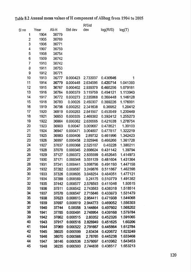
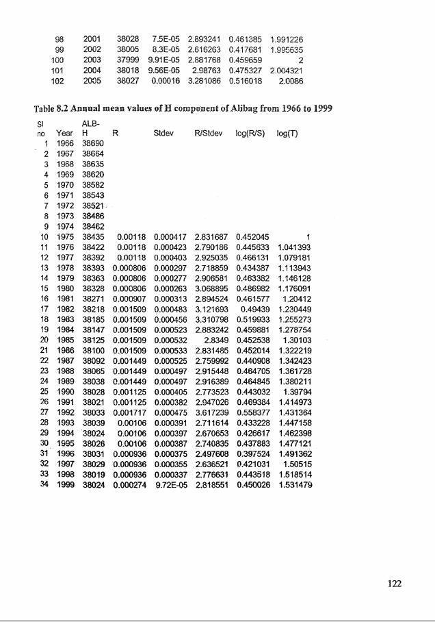
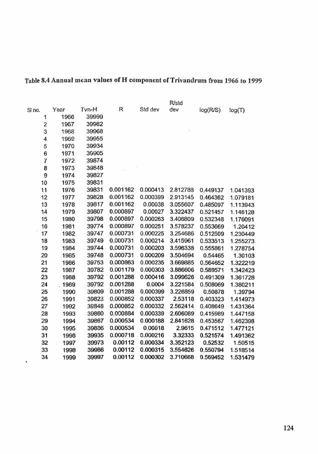
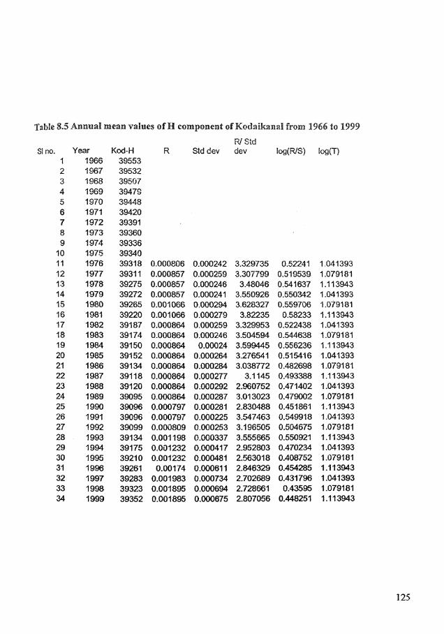
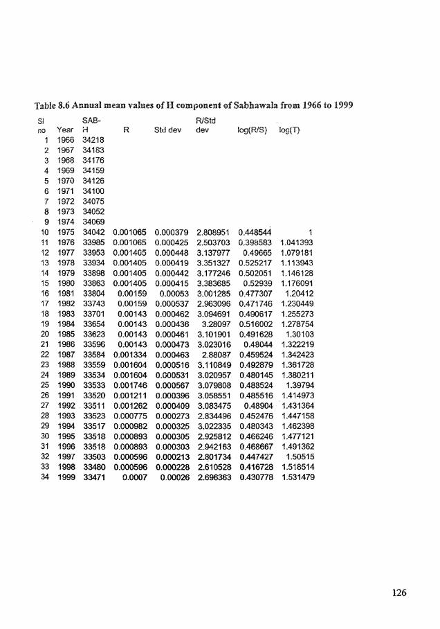
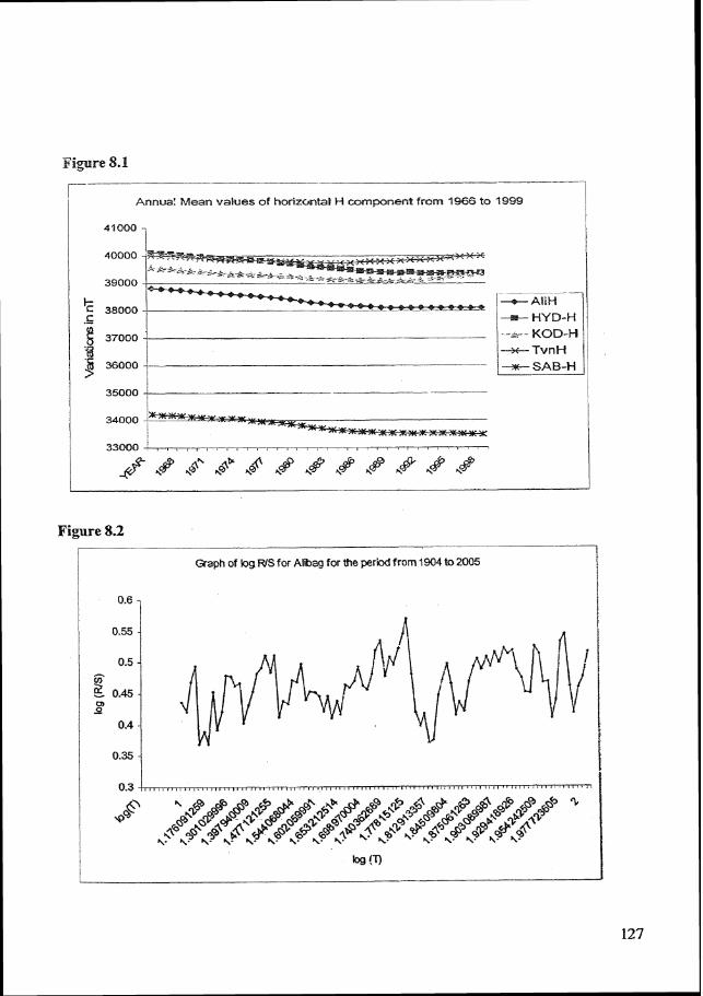
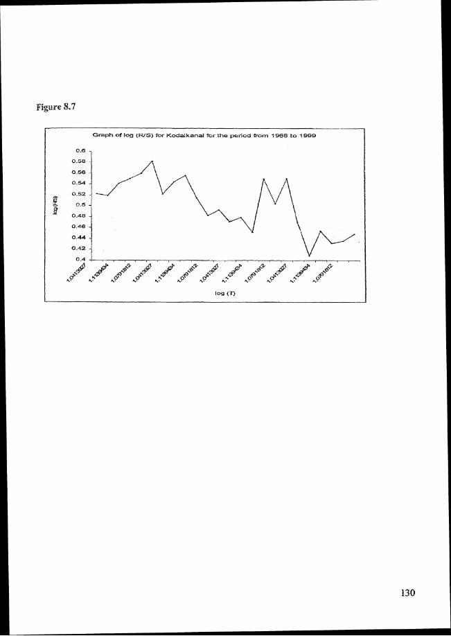
8.8 Application to geomagnetic annual variation in horfiontal component (El)

Annual mean values of the sensitive horizontal W component of the geomagnetic field

variations at the five observatories, Alibag, Hyderabad, Kodaikanal, Trivandrum and Sabhawala

are considered for this analysis. The data of Alibag observatory are available for 102 years from

1904 to 2005. For the other observatories the common data are available from 1966 to 1999 only.

These data are utilized for this study. The analysis is performed in 2 stages: Data on Alibag

observatory separately for 102 years are considered separately and the other observatories with

common data for 34 years are taken up.

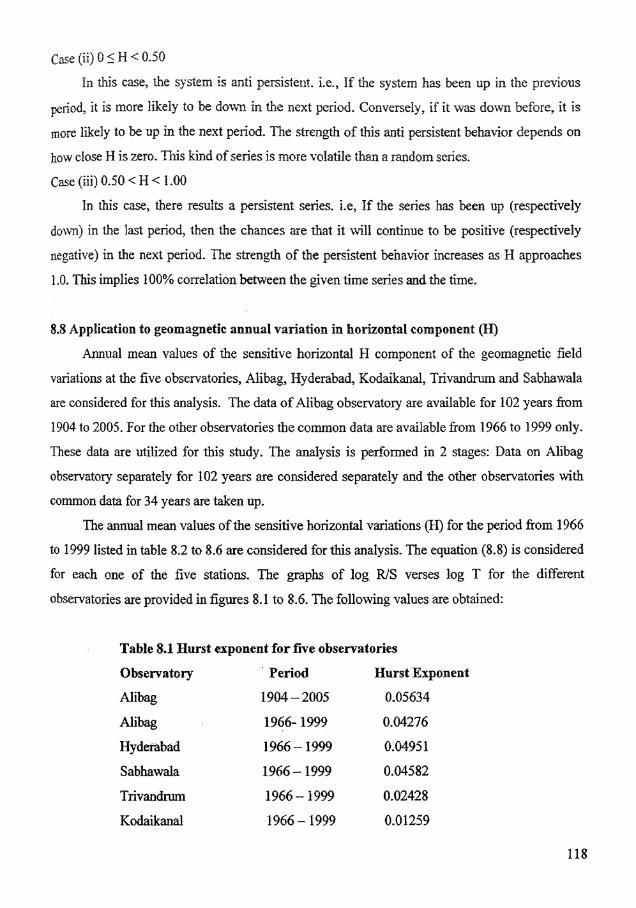
The annual mean values of the sensitive horizontal variations (H) for the period from 1966

to 1999 listed in table 8.2 to 8.6 are cansidered for this analysis. The equation (8.8) is considered

for each one of the five stations. The graphs of log R/S verses log T for the different

observatories are provided in figures 8.1 to 8.6. The following values are obtained:

Table 8.1 Hunt exponent for five observatories

Observatory Period Hurst Exponent

Alibag 1904 - 2005 0.05634

Alibag 1966- 1999 0.04276

Hyderabad 1966 - 1999 0.0495 1

Sabhawala 1966 - 1999 0.04582

Trivandm 1966 - I999 0.02428

Kodaikanal 1966 - 1999 0.01259

From the table 8.1, it is observed that the value of the Hwst Exponent (H) is less than 0.5

for all the observatories considered for this analysis.

'The results oblained i~ldicate that, the system is anti persistent, i.e., if the system has been

up in the previous period, it is more likely to be don3 in the next pe~od. Con~ersely, if it was

d o m before, it is more l&eIy to be up in the next period. The strength of this anti persistent

behavior depends on how close W is zero.

8.9 Csmcluslicm

The geomagnetic annual mean values of horizontal M component for rhe five observatories

andyzed in this chapter reveals the anti persistent behavior.

ma

Nm

Me

Nm

mN

b.

-m

~a

mN

mr

b

Nb

Ob

bN

tO

CO

mW

bb

O

W-

~V

~N

~~

N~

~O

~~

~%

~%

~%

%W

V)

I~

V)

~

%k

%~

~~

~~

$&

,m

$Y

8$$2 000

QO

OO

OQ

O 000000000000000000

4~

~8

qX

8g

gq

g$

~q

qq

3.

qq

qq

~q

8~

85

28

8~

~8

8~

i!

oaooo oooo oooooooooooooooo ooodddod

&&AA4AA4A'&A2AAAAAA44AAa4AA&AaAa&A~Aa&A&A&&AdaA~&~A

Bm

cw

c

wm

wc

g

gg

g

mw

wc

mw

om

mm

m~

ww

mg

gg

gg

C

~~

CO

CD

CD

QQ

W~

88

85

8#

~8

~9

~a

a~

m~

$8

W2

82

~Y

~2

X2

:2

~~

mo

3-

J~

)~

1B

8I

~8

~~

%~

~~

8~

~8

a

ow

w$

$o

ww

W~

~w

ww

ww

oW

w~

o

wg

gg

n

n~

g~

~a

W~

~~

~~

~~

~%

~~

~~

~~

~g

gg

gg

EO

1g

gQ

)g

qq

gm

gg

gg

ma

W

WN

~

~$

~q

@p

~g

q@

~~

gg

~~

~$

~~

~~

1~

~~

8~

~W

gg

~~

~~

g~

g~

gg

~~

~f

f~

~~

~

000~000000 000000000

PP

oo

PP

o Po

000000000000000008

oo

gg

ob

bb

bo

b

bo

oo

bo

ob

PP

oo

oo

oo

oP

oo

PP

oo

bo

bb

ob

bb

bo

bb

ir

so

bb

00 g*X0000000000

OO

OO

OO

*O

DO

O

00

0

00

00

00

00

00

00

00

gg0080gg

8$

P8

8g

g0

g8

8~

08

~~

g~

~8

g~

8~

~s

~~

~"

p~

g~

~~

~$

O~

~$

~

~~

19

$Q

a~

~#

ag

~g

g~

~$

g~

~g

~q

~~

~:

;;

]~

~~

~~

g~

g~

l;

it

;;

fq

~~

gg

~~

~~

~~

g

dA

fF

qA

,A

+F

A

AA

AA

AA

A

AA

&A

&A

AA

A&

&A

&A

& 42

-A

dd

dd

A&

d*

d

--

L-

.h

J

b$

pm

~

OW

~W

W

'

&&

&&

"+

~A

.q

~~

q+

kk

~.

..

,"

"

bk

nin

in

,Ql.

JA

2$

3

bb

bb

$g

gg

g$

~W

wd

"b

~m

k-

4Y

a0

1P

*W

N-

Jk

~*

a

-4

m

~R~~~

!3#f f f

$gw

&

%W

ag

W

QW

-4

AM

CO

NC

n~

NO

U'

N COBgCnWONP

-* R) IU

-J-i

MM

m

KIA

Pm

W

~w

wo

ao

~w

o3

~o

~~

o~

P~

~w

wo

)w

w(

oo

1~

wa

,-

L1

oo

~~

mo

Ia

w~

aw

~~

a~

~~

P

WW

~~

~~

~A

~O

NW

WA

p

,~~

e,~

oe

w,N

w,M

,,V

Io~

~Q

,gO

~~

03

W

FJ

WV

Io

O

-4

Ad

A

mO

mm

Nq

ma

m

io

w~

~~

~$

gg

~

W~

WW

WW

WW

W w

Ww

OW

WW

Ow

WW

wW

WW

WW

W

WW

W

tg

NN

NN

W

88

88

88

88

ss

~8

~2

22

2~

E$

8$

8f

%~

E~

%~

%%

8%

8P

~

88

88

8

g 7J

r?

. m

&W

N-

&d

OQ

OQ

QO

OO

OO

OO

OO

O

OO

P"

pO

Ob

bb

bb

bb

bb

bb

b~

bb

~~

p

8~

~~

s~

$"

~z

"~

zz

~g

8X

88

88

g

WW

WA

-A

-*

-d

P

uiu

iaU

lUl

W0

3m

AA

A

4W

WW

00

A

NN

A%

%O

OO

OQ

80

00

~-

-'

d

&~

mm

am

~4

ma

Qw

aw

wm

ww

4m

~~

07

am

r

k

ail 3

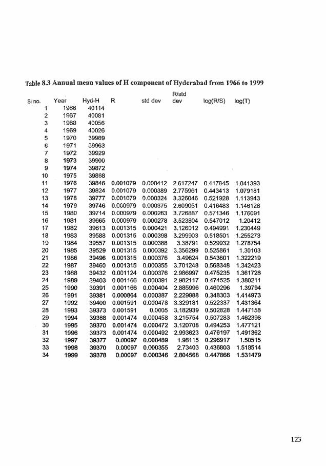
Table 8 3 Annual mean values of H compone~lt ef Hyderabad from $966 tc~ 19%

Wstd SI no. Year Hyd-H R std dev dev ~ w W S ? ~w(T)

1 1966 40114 2 1.967 40081 3 1968 40056 4 1969 40026 5 t970 39989 E 1971 39963 7 1972 39929 8 1973 39900 9 1974 39872

10 1975 39868 11 1976 39e46 0.001079 0.000412 2.617247 0.417845 1.041393 12 1977 39824 0.001079 0.000389 2.775961 0.443413 1.079181 13 1978 39777 0.001079 0.000324 3.326046 0.521928 1.1 13943 14 1979 39746 0.000979 0.000375 2.609051 0.416483 1.146128 15 1980 39714 0.000979 0.000263 3.726887 0.571346 1 .I76091 16 1981 39665 0.000979 0.000278 3.523804 0.547012 1.20412 17 1982 39613 0.001315 0.000421 3.126012 0.494991 1.230449 18 1983 39588 0.001315 0.000398 3.299903 0.518501 1.255273 19 1984 39557 0.001315 0.000388 3.38791 0.529932 1.278754 20 1985 39529 0.001 315 0.000392 3.356299 0.525861 1.30103 21 1986 39496 0.001315 0.000376 3.49624 0.543601 1.322219 22 1987 39460 0.001315 0.000355 3.701248 0.568348 1.342423 23 1988 39432 0.001124 0.000376 2.986997 0.475235 1.361728 24 1989 39403 0.001 166 0.000391 2.9821 17 0.474525 1.38021 1 25 1990 39391 0.001166 0.000404 2.885996 0.460296 1.39794 26 1991 39381 0.000864 0.000387 2.229988 0.348303 1.414973 27 1992 39400 0.001591 0.000478 3.329181 0.522337 1.431364 28 1993 39373 0.001591 0.0005 3.182939 0.502828 2.447158 29 1994 39368 0.001474 0.000458 3.215754 0.507283 1.462398 30 1995 39370 0.001474 0.000472 3.120708 0.494253 1.477121 31 1996 39373 0.001474 0.000492 2.993623 0.476197 1.491362 32 1997 39377 0.170097 0.000489 1.98115 0.296917 1.50515 33 1998 39370 0.00097 0.000355 2.73403 0.436803 1.518514 34 1999 39378 0.00097 0.000346 2.804568 (3.447866 1.531479

Tabjle 8.4 Annual anfan vdaes of H component oPTrivandrtam from 1966 to 1999

Si no. Y 1 2 3 4 5 6 7 8 9

10 11 12 13 14 15 16 17 18 13 20 21 22 23 24 25 26 27 28 29 30 31 32 33 34

ear 1966 1967 1968 1960 1970 1971 1972 1973 1 974 1975 1976 1977 1978 1979 1980 1981 1982 1983 1 984 1985 1986 1987 1988 1989 1990 1991 1 992 1993 1994 1995 1995 1997 1998 1999

Std dev

0.00041 3 0.000399 0.00038 0.00027

0.000263 0.000251 0.000225 0.000214 0.000203 0.000209 0.000235 0.000303 0.000416

0.0004 0.000399 0.000337 0.000332 0.000339 0.000188 0 00018

3.000216 0.000334 0.00031 5 0.000302

Ristd dev

2.812788 2.913145 3.055607 3.322437 3.406809 3.578237 3.254686 3.415961 3.596338 3.504694 3.669885 3.886606 3.099626 3.221584 3.226859 2.531 18

2.562414 2.606089 2.841628

2.961 5 3.32333

3.3521 23 3.554626 3.71 0668

Tsble 8.6 Annual mean values of M component of Sabhawalan from 1966 to 1989

SI no Year

1 1966 2 1967 3 1968 4 1969 5 1979 6 1971 7 1972 8 1973 9 1974

10 1975 ?I 1976 12 1977 13 1978 14 1979 15 1980 16 1981 17 1982 18 1983 19 1984 20 1985 21 1986 22 1987 23 1988 24 1989 25 1990 26 1991 27 1992 28 1993 29 i994 30 1995 31 1996 32 I997 33 1998 34 1999

SAB- H 342 18 34 183 331 76 34159 341 26 34100 34075 34052 34069 34042 33985 33953 33934 33898 33863 33804 33743 33701 33654 33623 33596 33584 33559 33534 33533 33520 3351 1 33523 3351 7 33518 33518 33503 33480 33471

WStd Std dev dev

Annua: Mean values of horizontat H component from 1 9 6 6 to 1999

Figure 8.2

Graph of log WS for Aliag for the period from 1904 to 2005 i

Figure 8 3

Figure 8.4

r

Graph of log Ws for Hyderabad for the period from 1966 to 1999

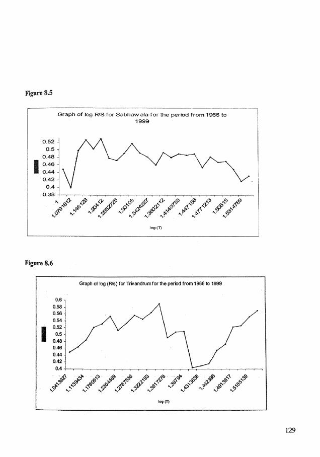
Graph of b g WS for Sabhaw tala for the period from 1966 to 1999

Figure 8.6

1 Graph of log (WS) fo r M-ikztsmal for the period from 1986 to 1999 -1