Chapter 8

Eigenvalues

So far, our applications have concentrated on statics: unchanging equilibrium config-urations of physical systems, including mass/spring chains, circuits, and structures, thatare modeled by linear systems of algebraic equations. It is now time to set our universein motion. In general, a dynamical system refers to the (differential) equations governingthe temporal behavior of some physical system: mechanical, electrical, chemical, fluid, etc.Our immediate goal is to understand the behavior of the simplest class of linear dynam-ical systems — first order autonomous linear systems of ordinary differential equations.As always, complete analysis of the linear situation is an essential prerequisite to makingprogress in the vastly more complicated nonlinear realm.

We begin with a very quick review of the scalar case, where solutions are simpleexponential functions. We use the exponential form of the scalar solution as a template fora possible solution in the vector case. Substituting the resulting formula into the systemleads us immediately to the equations defining the so-called eigenvalues and eigenvectors ofthe coefficient matrix. Further developments will require that we become familiar with thebasic theory of eigenvalues and eigenvectors, which prove to be of absolutely fundamentalimportance in both the mathematical theory and its applications, including numericalalgorithms.

The present chapter develops the most important properties of eigenvalues and eigen-vectors. The applications to dynamical systems will appear in Chapter 9, while applicationsto iterative systems and numerical methods is the topic of Chapter 10. Extensions of theeigenvalue concept to differential operators acting on infinite-dimensional function space,of essential importance for solving linear partial differential equations modelling continuousdynamical systems, will be covered in later chapters.Each square matrix has a collection ofone or more complex scalars called eigenvalues and associated vectors, called eigenvectors.Viewing the matrix as a linear transformation, the eigenvectors indicate directions of purestretch and the eigenvalues the degree of stretching. Most matrices are complete, meaningthat their (complex) eigenvectors form a basis of the underlying vector space. When ex-pressed in terms of its eigenvector basis, the matrix assumes a very simple diagonal form,and the analysis of its properties becomes extremely simple. A particularly important classare the symmetric matrices, whose eigenvectors form an orthogonal basis of R

n; in fact,this is by far the most common way for orthogonal bases to appear. Incomplete matricesare trickier, and we relegate them and their associated non-diagonal Jordan canonical formto the final section. The numerical computation of eigenvalues and eigenvectors is a chal-lenging issue, and must be be deferred until Section 10.6. Note: Unless you are prepared toconsult that section now, solving the computer-based problems in this chapter will require

4/6/04 267 c© 2004 Peter J. Olver

access to a computer package that can accurately compute eigenvalues and eigenvectors.

A non-square matrix A does not have eigenvalues. As an alternative, the squareroots of the eigenvalues of associated square Gram matrix K = AT A serve to define itssingular values. Singular values and principal component analysis appear in an increasinglybroad range of modern applications, including statistics, data mining, image processing,semantics, language and speech recognition, and learning theory. The singular values areused to define the condition number of a matrix, quantifying the difficulty of accuratelysolving an associated linear system.

8.1. Simple Dynamical Systems.

The purpose of this section is to motivate the concepts of eigenvalue and eigenvectorby attempting to solve the simplest class of dynamical systems — first order homogeneouslinear systems of ordinary differential equations. We begin with a review of the scalar case,introducing basic notions of stability in preparation for the general version, to be treatedin depth in Chapter 9. Readers who are uninterested in such motivational material mayskip ahead to Section 8.2 without penalty.

Scalar Ordinary Differential Equations

Consider the elementary scalar ordinary differential equation

du

dt= au. (8.1)

Here a ∈ R is a real constant, while the unknown u(t) is a scalar function. As you learnedin first year calculus, the general solution to (8.1) is an exponential function

u(t) = c eat. (8.2)

The integration constant c is uniquely determined by a single initial condition

u(t0) = b (8.3)

imposed at an initial time t0. Substituting t = t0 into the solution formula (8.2),

u(t0) = c eat0 = b, and so c = b e−at0 .

We conclude thatu(t) = b ea(t−t0). (8.4)

is the unique solution to the scalar initial value problem (8.1), (8.3).

Example 8.1. The radioactive decay of an isotope, say Uranium 238, is governedby the differential equation

du

dt= − γ u. (8.5)

Here u(t) denotes the amount of the isotope remaining at time t, and the coefficientγ > 0 governs the decay rate. The solution is given by an exponentially decaying functionu(t) = c e−γ t, where c = u(0) is the initial amount of radioactive material.

4/6/04 268 c© 2004 Peter J. Olver

-1 -0.5 0.5 1

-6

-4

-2

2

4

6

a < 0

-1 -0.5 0.5 1

-6

-4

-2

2

4

6

a = 0

-1 -0.5 0.5 1

-6

-4

-2

2

4

6

a > 0

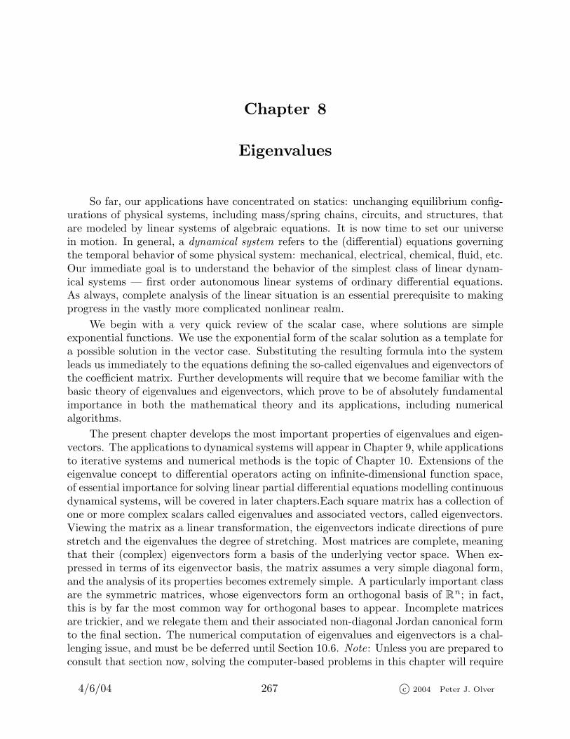
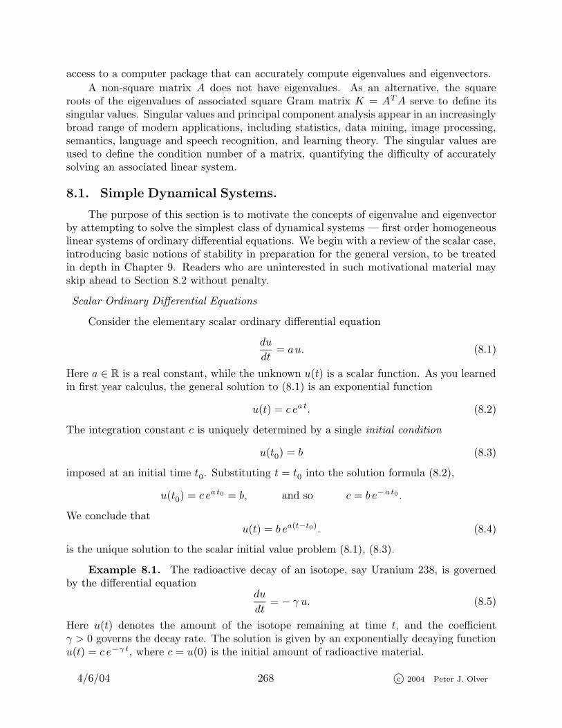
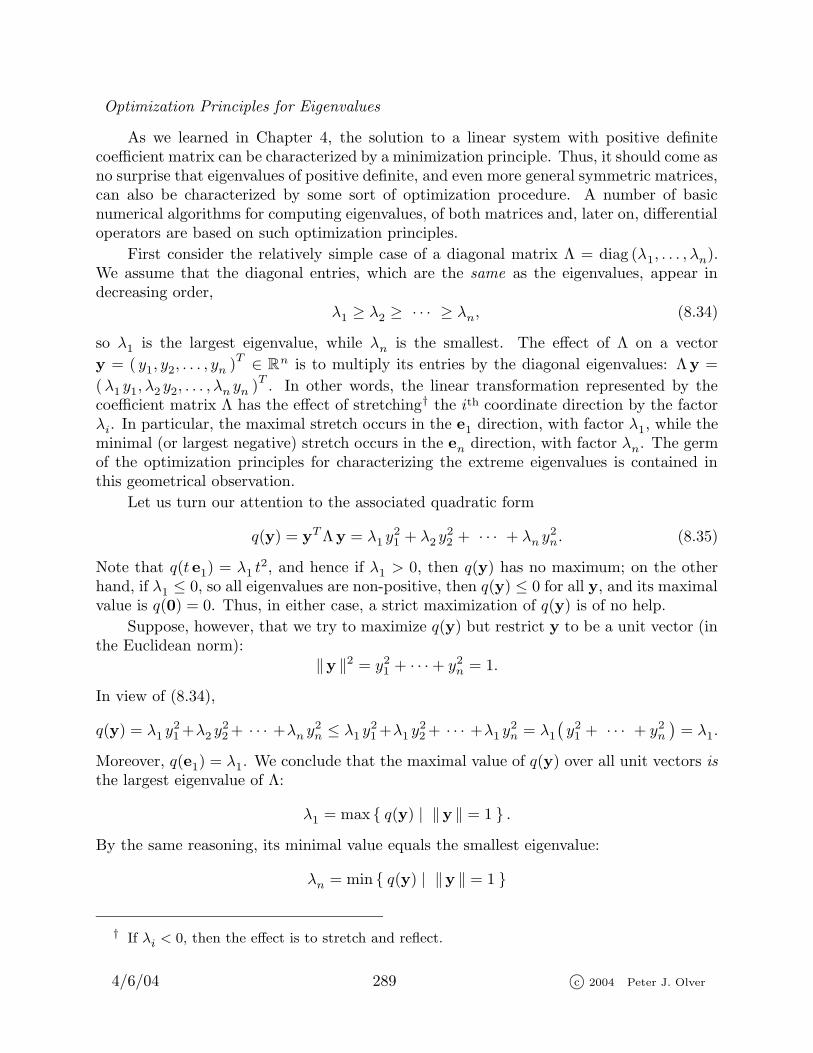
Figure 8.1. Solutions to¦

u = a u.

The isotope’s half-life t? is the time it takes for half of a sample to decay, that is whenu(t?) = 1

2 u(0). To determine t?, we solve the algebraic equation

e−γ t?

= 12 , so that t? =

log 2

γ. (8.6)

Let us make some elementary, but pertinent observations about this simple lineardynamical system. First of all, since the equation is homogeneous, the zero functionu(t) ≡ 0 (corresponding to c = 0) is a constant solution, known as an equilibrium solution

or fixed point , since it does not depend on t. If the coefficient a > 0 is positive, then thesolutions (8.2) are exponentially growing (in absolute value) as t → +∞. This implies thatthe zero equilibrium solution is unstable. The initial condition u(t0) = 0 produces the zerosolution, but if we make a tiny error (either physical, numerical, or mathematical) in theinitial data, say u(t0) = ε, then the solution u(t) = ε ea(t−t0) will eventually get very faraway from equilibrium. More generally, any two solutions with very close, but not equal,initial data, will eventually become arbitrarily far apart: |u1(t) − u2(t) | → ∞ as t → ∞.One consequence is an inherent difficulty in accurately computing the long time behaviorof the solution, since small numerical errors will eventually have very large effects.

On the other hand, if a < 0, the solutions are exponentially decaying in time. In thiscase, the zero solution is stable, since a small error in the initial data will have a negligibleeffect on the solution. In fact, the zero solution is globally asymptotically stable. The phrase“asymptotically stable” implies that solutions that start out near equilibrium eventuallyreturn; more specifically, if u(t0) = ε is small, then u(t) → 0 as t → ∞. “Globally” impliesthat all solutions, no matter how large the initial data is, return to equilibrium. In fact, fora linear system, the stability of an equilibrium solution is inevitably a global phenomenon.

The borderline case is when a = 0. Then all the solutions to (8.1) are constant. In thiscase, the zero solution is stable — indeed, globally stable — but not asymptotically stable.The solution to the initial value problem u(t0) = ε is u(t) ≡ ε. Therefore, a solution thatstarts out near equilibrium will remain near, but will not asymptotically return. The threequalitatively different possibilities are illustrated in Figure 8.1.

First Order Dynamical Systems

The simplest class of dynamical systems consist of n first order ordinary differential

4/6/04 269 c© 2004 Peter J. Olver

equations for n unknown functions

du1

dt= f1(t, u1, . . . , un), . . .

dun

dt= fn(t, u1, . . . , un),

which depend on a scalar variable t ∈ R, which we usually view as time. We will oftenwrite the system in the equivalent vector form

du

dt= f(t,u). (8.7)

A vector-valued solution u(t) = (u1(t), . . . , un(t))T serves to parametrize a curve in Rn,

called a solution trajectory . A dynamical system is called autonomous if the time variablet does not appear explicitly on the right hand side, and so has the system has the form

du

dt= f(u). (8.8)

Dynamical systems of ordinary differential equations appear in an astonishing variety ofapplications, and have been the focus of intense research activity since the early days ofcalculus.

We shall concentrate most of our attention on the very simplest case: a homogeneous,linear, autonomous dynamical system

du

dt= Au, (8.9)

in which A is a constant n×n matrix. In full detail, the system consists of n linear ordinarydifferential equations

du1

dt= a11 u1 + a12 u2 + · · · + a1n un,

du2

dt= a21 u1 + a22 u2 + · · · + a2n un,

......

dun

dt= an1 u1 + an2 u2 + · · · + ann un,

(8.10)

involving n unknown functions u1(t), u2(t), . . . , un(t). In the autonomous case, the coeffi-cients aij are assumed to be (real) constants. We seek not only to develop basic solutiontechniques for such dynamical systems, but to also understand their behavior from both aqualitative and quantitative standpoint.

Drawing our inspiration from the exponential solution formula (8.2) in the scalar case,let us investigate whether the vector system admits any solutions of a similar exponentialform

u(t) = eλt v. (8.11)

Here λ is a constant scalar, so eλt is a scalar function of t, while v ∈ Rn is a constant vector.

In other words, the components ui(t) = vi eλt of our desired solution are assumed to be

4/6/04 270 c© 2004 Peter J. Olver

constant multiples of the same exponential function. Since v is assumed to be constant,the derivative of u(t) is easily found:

du

dt=

d

dt

(eλt v

)= λ eλt v.

On the other hand, since eλt is a scalar, it commutes with matrix multiplication, and so

Au = Aeλt v = eλtAv.

Therefore, u(t) will solve the system (8.9) if and only if

λ eλt v = eλtAv,

or, canceling the common scalar factor eλt,

λv = Av.

The result is a system of algebraic equations relating the vector v and the scalar λ. Analysisof this system and its ramifications will be the topic of the remainder of this chapter.After gaining a complete understanding, we will return, suitably armed, to the main issue,solution of linear dynamical systems, in Chapter 9.

8.2. Eigenvalues and Eigenvectors.

We inaugurate our discussion of eigenvalues and eigenvectors with the fundamentaldefinition.

Definition 8.2. Let A be an n × n matrix. A scalar λ is called an eigenvalue of Aif there is a non-zero vector v 6= 0, called an eigenvector , such that

Av = λv. (8.12)

Thus, the matrix A effectively stretches the eigenvector v by an amount specified bythe eigenvalue λ. In this manner, the eigenvectors specify the directions of pure stretchfor the linear transformation defined by the matrix A.

Remark : The odd-looking terms “eigenvalue” and “eigenvector” are hybrid German–English words. In the original German, they are Eigenwert and Eigenvektor , which canbe fully translated as “proper value” and “proper vector”. For some reason, the half-translated terms have acquired a certain charm, and are now standard. The alternativeEnglish terms characteristic value and characteristic vector can be found in some (mostlyolder) texts. Oddly, the term characteristic equation, to be defined below, is still used.

The requirement that the eigenvector v be nonzero is important, since v = 0 is atrivial solution to the eigenvalue equation (8.12) for any scalar λ. Moreover, as far assolving linear ordinary differential equations goes, the zero vector v = 0 only gives thetrivial zero solution u(t) ≡ 0.

The eigenvalue equation (8.12) is a system of linear equations for the entries of theeigenvector v — provided the eigenvalue λ is specified in advance — but is “mildly”

4/6/04 271 c© 2004 Peter J. Olver

nonlinear as a combined system for λ and v. Gaussian elimination per se will not solvethe problem, and we are in need of a new idea. Let us begin by rewriting the equation inthe form

(A − λ I )v = 0, (8.13)

where I is the identity matrix of the correct size†. Now, for given λ, equation (8.13) is ahomogeneous linear system for v, and always has the trivial zero solution v = 0. But weare specifically seeking a nonzero solution! According to Theorem 1.45, a homogeneouslinear system has a nonzero solution v 6= 0 if and only if its coefficient matrix, which inthis case is A − λ I , is singular. This observation is the key to resolving the eigenvectorequation.

Theorem 8.3. A scalar λ is an eigenvalue of the n × n matrix A if and only if

the matrix A − λ I is singular, i.e., of rank < n. The corresponding eigenvectors are the

nonzero solutions to the eigenvalue equation (A − λ I )v = 0.

We know a number of ways to characterize singular matrices, including the vanishingdeterminant criterion given in (det0 ). Therefore, the following result is an immediatecorollary.

Proposition 8.4. A scalar λ is an eigenvalue of the matrix A if and only if λ is a

solution to the characteristic equation

det(A − λ I ) = 0. (8.14)

In practice, when finding eigenvalues and eigenvectors by hand, one first solves thecharacteristic equation (8.14). Then, for each eigenvalue λ one uses standard linear algebramethods, i.e., Gaussian elimination, to solve the corresponding linear system (8.13) for theeigenvector v.

Example 8.5. Consider the 2 × 2 matrix

A =

(3 11 3

).

We compute the determinant in the characteristic equation using (1.34):

det(A − λ I ) = det

(3 − λ 1

1 3 − λ

)= (3 − λ)2 − 1 = λ2 − 6λ + 8.

Thus, the characteristic equation is a quadratic polynomial equation, and can be solvedby factorization:

λ2 − 6λ + 8 = (λ − 4) (λ − 2) = 0.

We conclude that A has two eigenvalues: λ1 = 4 and λ2 = 2.

† Note that it is not legal to write (8.13) in the form (A− λ)v = 0 since we do not know howto subtract a scalar λ from a matrix A. Worse, if you type A − λ in Matlab, it will subtract λ

from all the entries of A, which is not what we are after!

4/6/04 272 c© 2004 Peter J. Olver

For each eigenvalue, the corresponding eigenvectors are found by solving the associatedhomogeneous linear system (8.13). For the first eigenvalue, the eigenvector equation is

(A − 4 I )v =

(−1 11 −1

)(xy

)=

(00

), or

−x + y = 0,

x − y = 0.

The general solution is

x = y = a, so v =

(aa

)= a

(11

),

where a is an arbitrary scalar. Only the nonzero solutions† count as eigenvectors, and sothe eigenvectors for the eigenvalue λ1 = 4 must have a 6= 0, i.e., they are all nonzero scalar

multiples of the basic eigenvector v1 = ( 1, 1 )T.

Remark : In general, if v is an eigenvector of A for the eigenvalue λ, then so is anynonzero scalar multiple of v. (Why?) In practice, we only distinguish linearly independent

eigenvectors. Thus, in this example, we shall say “v1 = ( 1, 1 )T

is the eigenvector corre-sponding to the eigenvalue λ1 = 4”, when we really mean that the eigenvectors for λ1 = 4consist of all nonzero scalar multiples of v1.

Similarly, for the second eigenvalue λ2 = 2, the eigenvector equation is

(A − 2 I )v =

(1 11 1

)(xy

)=

(00

).

The solution (−a, a )T

= a (−1, 1 )T

is the set of scalar multiples of the eigenvector

v2 = (−1, 1 )T. Therefore, the complete list of eigenvalues and eigenvectors (up to scalar

multiple) is

λ1 = 4, v1 =

(11

), λ2 = 2, v2 =

(−11

).

Example 8.6. Consider the 3 × 3 matrix

A =

0 −1 −11 2 11 1 2

.

† If, at this stage, you end up with a linear system with only the trivial zero solution, you’vedone something wrong! Either you don’t have a correct eigenvalue — maybe you made a mistakesetting up and/or solving the characteristic equation — or you’ve made an error solving thehomogeneous eigenvector system.

4/6/04 273 c© 2004 Peter J. Olver

Using the formula (1.82) for a 3 × 3 determinant, we compute the characteristic equation

0 = det(A − λ I ) = det

−λ −1 −11 2 − λ 11 1 2 − λ

= (−λ)(2 − λ)2 + (−1) · 1 · 1 + (−1) · 1 · 1 −− 1 · (2 − λ)(−1) − 1 · 1 · (−λ) − (2 − λ) · 1 · (−1)

= −λ3 + 4λ2 − 5λ + 2.

The resulting cubic polynomial can be factorized:

−λ3 + 4λ2 − 5λ + 2 = − (λ − 1)2 (λ − 2) = 0.

Most 3× 3 matrices have three different eigenvalues, but this particular one has only two:λ1 = 1, which is called a double eigenvalue since it is a double root of the characteristicequation, along with a simple eigenvalue λ2 = 2.

The eigenvector equation (8.13) for the double eigenvalue λ1 = 1 is

(A − I )v =

−1 −1 −11 1 11 1 1

xyz

=

000

.

The general solution to this homogeneous linear system

v =

−a − bab

= a

−110

+ b

−101

depends upon two free variables: y = a, z = b. Any nonzero solution forms a valideigenvector for the eigenvalue λ1 = 1, and so the general eigenvector is any non-zero linear

combination of the two “basis eigenvectors” v1 = (−1, 1, 0 )T, v1 = (−1, 0, 1 )

T.

On the other hand, the eigenvector equation for the simple eigenvalue λ2 = 2 is

(A − 2 I )v =

−2 −1 −11 0 11 1 0

xyz

=

000

.

The general solution

v =

−aaa

= a

−111

consists of all scalar multiple of the eigenvector v2 = (−1, 1, 1 )T.

4/6/04 274 c© 2004 Peter J. Olver

In summary, the eigenvalues and (basis) eigenvectors for this matrix are

λ1 = 1, v1 =

−110

, v1 =

−101

,

λ2 = 2, v2 =

−111

.

(8.15)

In general, given an eigenvalue λ, the corresponding eigenspace Vλ ⊂ Rn is the sub-

space spanned by all its eigenvectors. Equivalently, the eigenspace is the kernel

Vλ = ker(A − λ I ). (8.16)

In particular, λ is an eigenvalue if and only if Vλ 6= {0} is a nontrivial subspace, and thenevery nonzero element of Vλ is a corresponding eigenvector. The most economical way toindicate each eigenspace is by writing out a basis, as in (8.15).

Example 8.7. The characteristic equation of the matrix A =

1 2 11 −1 12 0 1

is

0 = det(A − λ I ) = −λ3 + λ2 + 5λ + 3 = − (λ + 1)2 (λ − 3).

Again, there is a double eigenvalue λ1 = −1 and a simple eigenvalue λ2 = 3. However, inthis case the matrix

A − λ1 I = A + I =

2 2 11 0 12 0 2

has only a one-dimensional kernel, spanned by ( 2,−1,−2 )T. Thus, even though λ1 is a

double eigenvalue, it only admits a one-dimensional eigenspace. The list of eigenvaluesand eigenvectors is, in a sense, incomplete:

λ1 = −1, v1 =

2−1−2

, λ2 = 3, v2 =

212

.

Example 8.8. Finally, consider the matrix A =

1 2 00 1 −22 2 −1

. The characteristic

equation is

0 = det(A − λ I ) = −λ3 + λ2 − 3λ − 5 = − (λ + 1) (λ2 − 2λ + 5).

The linear factor yields the eigenvalue −1. The quadratic factor leads to two complexroots, 1 + 2 i and 1 − 2 i , which can be obtained via the quadratic formula. Hence A hasone real and two complex eigenvalues:

λ1 = −1, λ2 = 1 + 2 i , λ3 = 1 − 2 i .

4/6/04 275 c© 2004 Peter J. Olver

Complex eigenvalues are as important as real eigenvalues, and we need to be able to handlethem too. To find the corresponding eigenvectors, which will also be complex, we needto solve the usual eigenvalue equation (8.13), which is now a complex homogeneous linearsystem. For example, the eigenvector(s) for λ2 = 1 + 2 i are found by solving

(A − (1 + 2 i I

)v =

−2 i 2 00 −2 i −22 2 −2 − 2 i

xyz

=

000

.

This linear system can be solved by Gaussian elimination (with complex pivots). A simplerapproach is to work directly: the first equation −2 ix + 2y = 0 tells us that y = ix, whilethe second equation −2 i y − 2z = 0 says z = − i y = x. If we trust our calculationsso far, we do not need to solve the final equation 2x + 2y + (−2 − 2 i )z = 0, since weknow that the coefficient matrix is singular and hence it must be a consequence of the firsttwo equations. (However, it does serve as a useful check on our work.) So, the general

solution v = (x, ix, x )T

is an arbitrary constant multiple of the complex eigenvector

v2 = ( 1, i , 1 )T. The eigenvector equation for λ3 = 1− 2 i is similarly solved for the third

eigenvector v3 = ( 1,− i , 1 )T.

Summarizing, the matrix under consideration has three complex eigenvalues and threecorresponding eigenvectors, each unique up to (complex) scalar multiple:

λ1 = −1, λ2 = 1 + 2 i , λ3 = 1 − 2 i ,

v1 =

−111

, v2 =

1i1

, v3 =

1− i1

.

Note that the third complex eigenvalue is the complex conjugate of the second, and theeigenvectors are similarly related. This is indicative of a general fact for real matrices:

Proposition 8.9. If A is a real matrix with a complex eigenvalue λ = µ + i ν and

corresponding complex eigenvector v = x+ iy, then the complex conjugate λ = µ− i ν is

also an eigenvalue with complex conjugate eigenvector v = x − iy.

Proof : First take complex conjugates of the eigenvalue equation (8.12):

A v = Av = λv = λ v.

Using the fact that a real matrix is unaffected by conjugation, so A = A, we concludeAv = λv, which is the eigenvalue equation for the eigenvalue λ and eigenvector v. Q.E.D.

As a consequence, when dealing with real matrices, one only needs to compute theeigenvectors for one of each complex conjugate pair of eigenvalues. This observation ef-fectively halves the amount of work in the unfortunate event that we are confronted withcomplex eigenvalues.

Remark : The reader may recall that we said one should never use determinants inpractical computations. So why have we reverted to using determinants to find eigenvalues?The truthful answer is that the practical computation of eigenvalues and eigenvectors never

4/6/04 276 c© 2004 Peter J. Olver

resorts to the characteristic equation! The method is fraught with numerical traps andinefficiencies when (a) computing the determinant leading to the characteristic equation,then (b) solving the resulting polynomial equation, which is itself a nontrivial numericalproblem, [30], and, finally, (c) solving each of the resulting linear eigenvector systems.

Indeed, if we only know an approximation λ to the true eigenvalue λ, the approximateeigenvector system (A − λ)v = 0 has a nonsingular coefficient matrix, and hence onlyadmits the trivial solution — which does not even qualify as an eigenvector! Nevertheless,the characteristic equation does give us important theoretical insight into the structureof the eigenvalues of a matrix, and can be used on small, e.g., 2 × 2 and 3 × 3, matrices,when exact arithmetic is employed. Numerical algorithms for computing eigenvalues andeigenvectors are based on completely different ideas, and will be discussed in Section 10.6.

Basic Properties of Eigenvalues

If A is an n × n matrix, then its characteristic polynomial is

pA(λ) = det(A − λ I ) = cn λn + cn−1 λn−1 + · · · + c1 λ + c0. (8.17)

The fact that pA(λ) is a polynomial of degree n is a consequence of the general determi-nantal formula (1.81). Indeed, every term is plus or minus a product of n matrix entriescontaining one from each row and one from each column. The term corresponding to theidentity permutation is obtained by multiplying the diagonal entries together, which, inthis case, is

(a11−λ) (a22−λ) · · · (ann−λ) = (−1)nλn+(−1)n−1(a11 + a22 + · · · + ann

)λn−1+ · · · .

(8.18)All of the other terms have at most n− 2 diagonal factors aii − λ, and so are polynomialsof degree ≤ n − 2 in λ. Thus, (8.18) is the only summand containing the monomials λn

and λn−1, and so their respective coefficients are

cn = (−1)n, cn−1 = (−1)n−1(a11 + a22 + · · · + ann) = (−1)n−1 trA, (8.19)

where trA, the sum of its diagonal entries, is called the trace of the matrix A. The othercoefficients cn−2, . . . , c1, c0 in (8.17) are more complicated combinations of the entries ofA. However, setting λ = 0 implies pA(0) = detA = c0, and hence the constant termin the characteristic polynomial equals the determinant of the matrix. In particular, if

A =

(a bc d

)is a 2 × 2 matrix, its characteristic polynomial has the form

pA(λ) = det(A − λ I ) = det

(a − λ b

c d − λ

)

= λ2 − (a + d)λ + (ad − bc) = λ2 − (trA)λ + (detA).

(8.20)

As a result of these considerations, the characteristic equation of an n × n matrix Ais a polynomial equation of degree n. According to the Fundamental Theorem of Algebra(see Corollary 16.63) every (complex) polynomial of degree n can be completely factored:

pA(λ) = (−1)n(λ − λ1)(λ − λ2) · · · (λ − λn). (8.21)

4/6/04 277 c© 2004 Peter J. Olver

The complex numbers λ1, . . . , λn, some of which may be repeated, are the roots of thecharacteristic equation pA(λ) = 0, and hence the eigenvalues of the matrix A. Therefore,we immediately conclude:

Theorem 8.10. An n×n matrix A has at least one and at most n distinct complex

eigenvalues.

Most n×n matrices — meaning those for which the characteristic polynomial factorsinto n distinct factors — have exactly n complex eigenvalues. More generally, an eigenvalueλj is said to have multiplicity m if the factor (λ − λj) appears exactly m times in thefactorization (8.21) of the characteristic polynomial. An eigenvalue is simple if it hasmultiplicity 1. In particular, A has n distinct eigenvalues if and only if all its eigenvalues aresimple. In all cases, when the eigenvalues are counted in accordance with their multiplicity,every n × n matrix has a total of n possibly repeated eigenvalues.

An example of a matrix with just one eigenvalue, of multiplicity n, is the n×n identitymatrix I , whose only eigenvalue is λ = 1. In this case, every nonzero vector in R

n is aneigenvector of the identity matrix, and so the eigenspace is all of R

n. At the other extreme,the “bidiagonal” Jordan block matrix

Jλ =

λ 1λ 1

λ 1. . .

. . .

λ 1λ

, (8.22)

also has only one eigenvalue, λ, again of multiplicity n. But in this case, Jλ has only oneeigenvector (up to scalar multiple), which is the first standard basis vector e1, and so itseigenspace is one-dimensional. (You are asked to prove this in Exercise .)

Remark : If λ is a complex eigenvalue of multiplicity k for the real matrix A, then itscomplex conjugate λ also has multiplicity k. This is because complex conjugate roots of areal polynomial necessarily appear with identical multiplicities.

Remark : If n ≤ 4, then one can, in fact, write down an explicit formula for thesolution to a polynomial equation of degree n, and hence explicit (but not particularlyhelpful) formulae for the eigenvalues of general 2 × 2, 3 × 3 and 4 × 4 matrices. As soonas n ≥ 5, there is no explicit formula (at least in terms of radicals), and so one mustusually resort to numerical approximations. This remarkable and deep algebraic resultwas proved by the young Norwegian mathematician Nils Hendrik Abel in the early part ofthe nineteenth century, [59].

If we explicitly multiply out the factored product (8.21) and equate the result to thecharacteristic polynomial (8.17), we find that its coefficients c0, c1, . . . cn−1 can be writtenas certain polynomials of the roots, known as the elementary symmetric polynomials. Thefirst and last are of particular importance:

c0 = λ1 λ2 · · · λn, cn−1 = (−1)n−1 (λ1 + λ2 + · · · + λn). (8.23)

4/6/04 278 c© 2004 Peter J. Olver

Comparison with our previous formulae for the coefficients c0 and cn−1 leads to the fol-lowing useful result.

Proposition 8.11. The sum of the eigenvalues of a matrix equals its trace:

λ1 + λ2 + · · · + λn = tr A = a11 + a22 + · · · + ann. (8.24)

The product of the eigenvalues equals its determinant:

λ1 λ2 · · · λn = det A. (8.25)

Remark : For repeated eigenvalues, one must add or multiply them in the formulae(8.24), (8.25) according to their multiplicity.

Example 8.12. The matrix A =

1 2 11 −1 12 0 1

considered in Example 8.7 has trace

and determinant

tr A = 1, detA = 3.

These fix, respectively, the coefficient of λ2 and the constant term in the characteristicequation. This matrix has two distinct eigenvalues: −1, which is a double eigenvalue, and3, which is simple. For this particular matrix, formulae (8.24), (8.25) become

1 = trA = (−1) + (−1) + 3, 3 = detA = (−1)(−1) 3.

Note that the double eigenvalue contributes twice to the sum and product.

8.3. Eigenvector Bases and Diagonalization.

Most of the vector space bases that play a distinguished role in applications consist ofeigenvectors of a particular matrix. In this section, we show that the eigenvectors for any“complete” matrix automatically form a basis for R

n or, in the complex case, Cn. In the

following subsection, we use the eigenvector basis to rewrite the linear transformation de-termined by the matrix in a simple diagonal form. The most important case — symmetricand positive definite matrices — will be treated in the next section.

The first task is to show that eigenvectors corresponding to distinct eigenvalues areautomatically linearly independent.

Lemma 8.13. If λ1, . . . , λk are distinct eigenvalues of the same matrix A, then the

corresponding eigenvectors v1, . . . ,vk are linearly independent.

Proof : The reulst is proved by induction on the number of eigenvalues. The casek = 1 is immediate since an eigenvector cannot be zero. Assume that we know the resultis valid for k − 1 eigenvalues. Suppose we have a vanishing linear combination:

c1v1 + · · · + ck−1 vk−1 + ck vk = 0. (8.26)

4/6/04 279 c© 2004 Peter J. Olver

Let us multiply this equation by the matrix A:

A(c1v1 + · · · + ck−1 vk−1 + ck vk

)= c1 Av1 + · · · + ck−1 Avk−1 + ck Avk

= c1 λ1v1 + · · · + ck−1 λk−1 vk−1 + ck λk vk = 0.

On the other hand, if we multiply the original equation by λk, we also have

c1 λk v1 + · · · + ck−1 λk vk−1 + ck λk vk = 0.

Subtracting this from the previous equation, the final terms cancel and we are left withthe equation

c1(λ1 − λk)v1 + · · · + ck−1(λk−1 − λk)vk−1 = 0.

This is a vanishing linear combination of the first k − 1 eigenvectors, and so, by ourinduction hypothesis, can only happen if all the coefficients are zero:

c1(λ1 − λk) = 0, . . . ck−1(λk−1 − λk) = 0.

The eigenvalues were assumed to be distinct, so λj 6= λk when j 6= k. Consequently,c1 = · · · = ck−1 = 0. Substituting these values back into (8.26), we find ck vk = 0, andso ck = 0 also, since the eigenvector vk 6= 0. Thus we have proved that (8.26) holds ifand only if c1 = · · · = ck = 0, which implies the linear independence of the eigenvectorsv1, . . . ,vk. This completes the induction step. Q.E.D.

The most important consequence of this result is when a matrix has the maximumallotment of eigenvalues.

Theorem 8.14. If the n×n real matrix A has n distinct real eigenvalues λ1, . . . , λn,

then the corresponding real eigenvectors v1, . . . ,vn form a basis of Rn. If A (which may

now be either a real or a complex matrix) has n distinct complex eigenvalues, then the

corresponding eigenvectors v1, . . . ,vn form a basis of Cn.

If a matrix has multiple eigenvalues, then there may or may not be an eigenvectorbasis of R

n (or Cn). The matrix in Example 8.6 admits an eigenvector basis, whereas the

matrix in Example 8.7 does not. In general, it can be proved† that the dimension of theeigenspace is less than or equal to the eigenvalue’s multiplicity. In particular, every simpleeigenvalue has a one-dimensional eigenspace, and hence, up to scalar multiple, only oneassociated eigenvector.

Definition 8.15. An eigenvalue λ of a matrix A is called complete if its eigenspaceVλ = ker(A− λ I ) has the same dimension as its multiplicity. The matrix A is complete ifall its eigenvalues are.

Note that a simple eigenvalue is automatically complete, since its eigenspace is theone-dimensional subspace spanned by the corresponding eigenvector. Thus, only multipleeigenvalues can cause a matrix to be incomplete.

† This is a consequence of Theorem 8.43.

4/6/04 280 c© 2004 Peter J. Olver

Remark : The multiplicity of an eigenvalue λi is sometimes referred to as its algebraic

multiplicity . The dimension of the eigenspace Vλ is its geometric multiplicity , and socompleteness requires that the two multiplicities are equal. The word “complete” is notcompletely standard; other common terms for such matrices are perfect , semi-simple and,as discussed below, diagonalizable.

Theorem 8.16. An n × n real or complex matrix A is complete if and only if its

eigenvectors span Cn. In particular, any n × n matrix that has n distinct eigenvalues is

complete.

Or, stated another way, a matrix is complete if and only if it admits an eigenvectorbasis of C

n. Most matrices are complete. Incomplete n × n matrices, which have fewerthan n linearly independent complex eigenvectors, are more tricky to deal with, and werelegate most of the messy details to Section 8.6.

Remark : We already noted that complex eigenvectors of a real matrix always appearin conjugate pairs: v = x ± iy. It can be shown that the real and imaginary partsof these vectors form a real basis for R

n. (See Exercise for the underlying principle.)

For instance, in Example 8.8, the complex eigenvectors are

101

± i

010

. The vectors

−111

,

101

,

010

, consisting of the real eigenvector and the real and imaginary parts

of the complex eigenvectors, form a basis for R3.

Diagonalization

Let L: Rn → Rn be a linear transformation on n-dimensional Euclidean space. As we

know, cf. Theorem 7.5, L is determined by multiplication by an n × n matrix. However,the matrix representing a given linear transformation will depend upon the choice of basisfor the underlying vector space R

n. Linear transformations having a complicated matrixrepresentation in terms of the standard basis e1, . . . , en may be considerably simplified bychoosing a suitably adapted basis v1, . . . ,vn. We are now in a position to understand howto effect such a simplification.

For example, the linear transformation L

(xy

)=

(x − y

2x + 4y

)studied in Example 7.19

is represented by the matrix A =

(1 −12 4

)— when expressed in terms of the standard

basis of R2. In terms of the alternative basis v1 =

(1−1

), v2 =

(1−2

), it is represented

by the diagonal matrix

(2 00 3

), indicating it has a simple stretching action on the new

basis vectors: Av1 = 2v1, Av2 = 3v2. Now we can understand the reason for thissimplification. The new basis consists of the two eigenvectors of the matrix A. Thisobservation is indicative of a general fact: representing a linear transformation in terms

4/6/04 281 c© 2004 Peter J. Olver

of an eigenvector basis has the effect of replacing its matrix representative by a simplediagonal form. The effect is to diagonalize the original coefficient matrix.

According to (7.26), if v1, . . . ,vn form a basis of Rn, then the corresponding matrix

representative of the linear transformation L[v ] = Av is given by the similar matrix

B = S−1AS, where S = (v1 v2 . . . vn )T

is the matrix whose columns are the basis

vectors. In the preceding example, S =

(1 1−1 −2

), and we find that S−1AS =

(2 00 3

)

is a diagonal matrix.

Definition 8.17. A square matrix A is called diagonalizable if there exists a nonsin-gular matrix S and a diagonal matrix Λ = diag (λ1, . . . , λn) such that

S−1AS = Λ. (8.27)

A diagonal matrix represents a linear transformation that simultaneously stretches†

in the direction of the basis vectors. Thus, every diagonalizable matrix represents a ele-mentary combination of (complex) stretching transformations.

To understand the diagonalization equation (8.27), we rewrite it in the equivalentform

AS = S Λ. (8.28)

Using the basic property (1.11) of matrix multiplication, one easily sees that the kth columnof this n × n matrix equation is given by

Avk = λkvk.

Therefore, the columns of S are necessarily eigenvectors, and the entries of the diagonalmatrix Λ are the corresponding eigenvalues! And, as a result, a diagonalizable matrixA must have n linearly independent eigenvectors, i.e., an eigenvector basis, to form thecolumns of the nonsingular diagonalizing matrix S. Since the diagonal form Λ contains theeigenvalues along its diagonal, it is uniquely determined up to a permutation of its entries.

Now, as we know, not every matrix has an eigenvector basis. Moreover, even when itexists, the eigenvector basis may be complex, in which case S is a complex matrix, and theentries of the diagonal matrix Λ are the complex eigenvalues. Thus, we should distinguishbetween complete matrices that are diagonalizable over the complex numbers and the morerestrictive class of matrices which can be diagonalized by a real matrix S.

Theorem 8.18. A matrix is complex diagonalizable if and only if it is complete. A

matrix is real diagonalizable if and only if it is complete and has all real eigenvalues.

† A negative diagonal entry represents the combination of a reflection and stretch. Complexentries correspond to a complex stretching transformation. See Section 7.2 for details.

4/6/04 282 c© 2004 Peter J. Olver

Example 8.19. The 3 × 3 matrix A =

0 −1 −11 2 11 1 2

considered in Example 8.5

has eigenvector basis

v1 =

−110

, v2 =

−101

, v3 =

−111

.

We assemble these to form the eigenvector matrix

S =

−1 −1 −11 0 10 1 1

and so S−1 =

−1 0 −1−1 −1 01 1 1

.

The diagonalization equation (8.27) becomes

S−1AS =

−1 0 −1−1 −1 01 1 1

0 −1 −11 2 11 1 2

−1 −1 −11 0 10 1 1

=

1 0 00 1 00 0 2

= Λ,

with the eigenvalues of A appearing on the diagonal of Λ, in the same order as the eigen-vectors.

Remark : If a matrix is not complete, then it cannot be diagonalized. A simple example

is a matrix of the form

(1 c0 1

)with c 6= 0, which represents a shear in the direction of

the x axis. Incomplete matrices will be the subject of the Section 8.6.

8.4. Eigenvalues of Symmetric Matrices.

Fortunately, the matrices that arise in most applications are complete and, in fact,possess some additional structure that ameliorates the calculation of their eigenvalues andeigenvectors. The most important class are the symmetric, including positive definite,matrices. In fact, not only are the eigenvalues of a symmetric matrix necessarily real, theeigenvectors always form an orthogonal basis of the underlying Euclidean space. In suchsituations, we can tap into the dramatic power of orthogonal bases that we developed inChapter 5. In fact, this is by far the most common way for orthogonal bases to appear —as the eigenvector bases of symmetric matrices.

Theorem 8.20. Let A = AT be a real symmetric n × n matrix, Then

(a) All the eigenvalues of A are real.

(b) Eigenvectors corresponding to distinct eigenvalues are orthogonal.

(c) There is an orthonormal basis of Rn consisting of n eigenvectors of A.

In particular, all symmetric matrices are complete.

We defer the proof of Theorem 8.20 until the end of this section.

4/6/04 283 c© 2004 Peter J. Olver

Remark : Orthogonality is with respect to the standard dot product on Rn. As we

noted in Section 7.5, the transpose or adjoint operation is intimately connected with thedot product. An analogous result holds for self-adjoint linear transformations on R

n; seeExercise for details.

Example 8.21. The 2 × 2 matrix A =

(3 11 3

)considered in Example 8.5 is sym-

metric, and so has real eigenvalues λ1 = 4 and λ2 = 2. You can easily check that the

corresponding eigenvectors v1 = ( 1, 1 )T

and v2 = (−1, 1 )T

are orthogonal: v1 · v2 = 0,and hence form on orthogonal basis of R

2. An orthonormal basis is provided by the uniteigenvectors

u1 =

(1√2

1√2

), u2 =

(− 1√

2

1√2

),

obtained by dividing each eigenvector by its length: uk = vk/‖vk ‖.

Example 8.22. Consider the symmetric matrix A =

5 −4 2−4 5 22 2 −1

. A straight-

forward computation produces its eigenvalues and eigenvectors:

λ1 = 9, λ2 = 3, λ3 = −3,

v1 =

1−10

, v2 =

111

, v3 =

11−2

.

As the reader can check, the eigenvectors form an orthogonal basis of R3. The orthonormal

eigenvector basis promised by Theorem 8.20 is obtained by dividing each eigenvector byits norm:

u1 =

1√2

− 1√2

0

, u2 =

1√3

1√3

1√3

, u3 =

1√6

1√6

− 2√6

.

We can characterize positive definite matrices by their eigenvalues.

Theorem 8.23. A symmetric matrix K = KT is positive definite if and only if all

of its eigenvalues are strictly positive.

Proof : First, if K > 0, then, by definition, xT K x > 0 for all nonzero vectors x ∈ Rn.

In particular, if x = v is an eigenvector with (necessarily real) eigenvalue λ, then

0 < vT Kv = vT (λv) = λ ‖v ‖2, (8.29)

which immediately proves that λ > 0. Conversely, suppose K has all positive eigenvalues.Let u1, . . . ,un be the orthonormal eigenvector basis of R

n guaranteed by Theorem 8.20,with Kuj = λj uj . Then, writing

x = c1u1 + · · · + cn un, we have K x = c1 λ1u1 + · · · + cn λn un.

4/6/04 284 c© 2004 Peter J. Olver

Therefore, using the orthonormality of the eigenvectors,

xT K x = (c1u1 + · · · + cn un) · (c1 λ1u1 + · · · + cn λn un) = λ1 c21 + · · · + λn c2

n > 0

for any x 6= 0, since only x = 0 has coordinates c1 = · · · = cn = 0. This proves that thatK is positive definite. Q.E.D.

Remark : The same proof shows that K is positive semi-definite if and only if all itseigenvalues satisfy λ ≥ 0. A positive semi-definite matrix that is not positive definiteadmits a zero eigenvalue and one or more null eigenvectors, i.e., solutions to Kv = 0.Every nonzero element 0 6= v ∈ ker K of the kernel is a null eigenvector.

Example 8.24. Consider the symmetric matrix K =

8 0 10 8 11 1 7

. Its characteristic

equation is

det(K − λ I) = −λ3 + 23λ2 − 174λ + 432 = −(λ − 9)(λ − 8)(λ − 6),

and so its eigenvalues are 9, 8 and 6. Since they are all positive, K is a positive definitematrix. The associated eigenvectors are

λ1 = 9, v1 =

111

, λ2 = 8, v2 =

−110

, λ3 = 6, v3 =

−1−12

.

Note that the eigenvectors form an orthogonal basis of R3, as guaranteed by Theorem 8.20.

As usual, we can construct an corresponding orthonormal eigenvector basis

u1 =

1√3

1√3

1√3

, u2 =

− 1√2

1√2

0

, u3 =

− 1√6

− 1√6

2√6

,

by dividing each eigenvector by its norm.

Proof of Theorem 8.20 : First recall that if A = AT is real, symmetric, then

(Av) · w = v · (Aw) for all v,w ∈ Cn, (8.30)

where we use the Euclidean dot product for real vectors and, more generally, the Hermitiandot product v · w = vT w when they are complex. (See Exercise .)

To prove property (a), suppose λ is a complex eigenvalue with complex eigenvectorv ∈ C

n. Consider the Hermitian dot product of the complex vectors Av and v:

(Av) · v = (λv) · v = λ ‖v ‖2.

On the other hand, by (8.30),

(Av) · v = v · (Av) = v · (λv) = vT λv = λ ‖v ‖2.

4/6/04 285 c© 2004 Peter J. Olver

Equating these two expressions, we deduce

λ ‖v ‖2 = λ ‖v ‖2.

Since v is an eigenvector, it is nonzero, v 6= 0, and so λ = λ. This proves that theeigenvalue λ is real.

To prove (b), suppose

Av = λv, Aw = µw,

where λ 6= µ are distinct real eigenvalues. Then, again by (8.30),

λv · w = (Av) · w = v · (Aw) = v · (µw) = µv · w,

and hence(λ − µ)v · w = 0.

Since λ 6= µ, this implies that v · w = 0 and hence the eigenvectors v,w are orthogonal.

Finally, the proof of (c) is easy if all the eigenvalues of A are distinct. Theorem 8.14implies that the eigenvectors form a basis of R

n, and part (b) proves they are orthogonal.(An alternative proof starts with orthogonality, and then applies Proposition 5.4 to provethat the eigenvectors form a basis.) To obtain an orthonormal basis, we merely divide theeigenvectors by their lengths: uk = vk/‖vk ‖, as in Lemma 5.2.

To prove (c) in general, we proceed by induction on the size n of the matrix A. Thecase of a 1 × 1 matrix is trivial. (Why?) Let A have size n × n. We know that A has atleast one eigenvalue, λ1, which is necessarily real. Let v1 be the associated eigenvector.Let

V ⊥ = { w ∈ Rn | v1 · w = 0 }

denote the orthogonal complement to the eigenspace Vλ1— the set of all vectors orthogonal

to the first eigenvector. Proposition 5.48 implies that dimV ⊥ = n − 1, and we choosean orthonormal basis y1, . . . ,yn−1. Now, if w is any vector in V ⊥, so is Aw since, bysymmetry,

v1 · (Aw) = vT1 Aw = (Av1)

T w = λ1vT1 w = λ1(v1 · w) = 0.

Thus, A defines a linear transformation on V ⊥, and is represented by a symmetric (n−1)×(n − 1) matrix with respect to the chosen orthonormal basis y1, . . . ,yn−1. Our induction

hypothesis implies that there is an orthonormal basis of V ⊥ consisting of eigenvectorsu2, . . . ,un of A. Appending the unit eigenvector u1 = v1/‖v1 ‖ to this collection willcomplete the orthonormal basis of R

n. Q.E.D.

The Spectral Theorem

Since a real, symmetric matrix admits an eigenvector basis, it is diagonalizable. More-over, since we can arrange that the eigenvectors form an orthonormal basis, the diagonal-izing matrix takes a particularly simple form. Recall that an n × n matrix Q is calledorthogonal if and only if its columns form an orthonormal basis of R

n. Alternatively, onecharacterizes orthogonal matrices by the condition Q−1 = QT , as in Definition 5.18.

4/6/04 286 c© 2004 Peter J. Olver

Therefore, when we use the orthonormal eigenvector basis in the diaognalization for-mula (8.27), the result is the Spectral Theorem that governs the diagonalization of sym-metric matrices.

Theorem 8.25. Let A be a real, symmetric matrix. Then there exists an orthogonal

matrix Q such that

A = QΛQ−1 = QΛQT , (8.31)

where Λ is a real diagonal matrix. The eigenvalues of A appear on the diagonal of Λ, while

the eigenvectors are the corresponding columns of Q.

Remark : The term “spectrum” refers to the eigenvalues of a matrix or, more generally,a linear operator. The terminology is motivated by physics. The spectral energy lines ofatoms, molecules and nuclei are characterized as the eigenvalues of the governing quantummechanical linear operators, [102, 106].

Warning : The spectral factorization A = QΛQT and the Gaussian factorization A =LDLT of a regular symmetric matrix, cf. (1.52), are completely different. In particular,the eigenvalues are not the pivots, so Λ 6= D.

The spectral decomposition (8.31) provides us with an alternative means of diagonal-izing the associated quadratic form q(x) = xT Ax, i.e., of completing the square. Wewrite

q(x) = xT Ax = xT QΛQT x = yT Λy =

n∑

i=1

λi y2i , (8.32)

where y = QT x = Q−1x are the coordinates of x with respect to the orthonormal eigen-value basis of A. In particular, q(x) > 0 for all x 6= 0 and so A is positive definite if andonly if each eigenvalue λi > 0 is strictly positive, reconfirming Theorem 8.23.

Example 8.26. For the 2 × 2 matrix A =

(3 11 3

)considered in Example 8.21,

the orthonormal eigenvectors produce the diagonalizing orthogonal rotation matrix Q =(1√2

− 1√2

1√2

1√2

). The reader can check the spectral factorization

(3 11 3

)= A = QΛQT =

(1√2

− 1√2

1√2

1√2

) (4 0

0 2

) (1√2

1√2

− 1√2

1√2

).

According to (8.32), the associated quadratic form is diagonalized as

q(x) = 3x21 + 2x1 x2 + 3x2

2 = 4y21 + 2y2

2 ,

where y = QT x, i.e., y1 =x1 + x2√

2, y2 =

−x1 + x2√2

.

4/6/04 287 c© 2004 Peter J. Olver

A

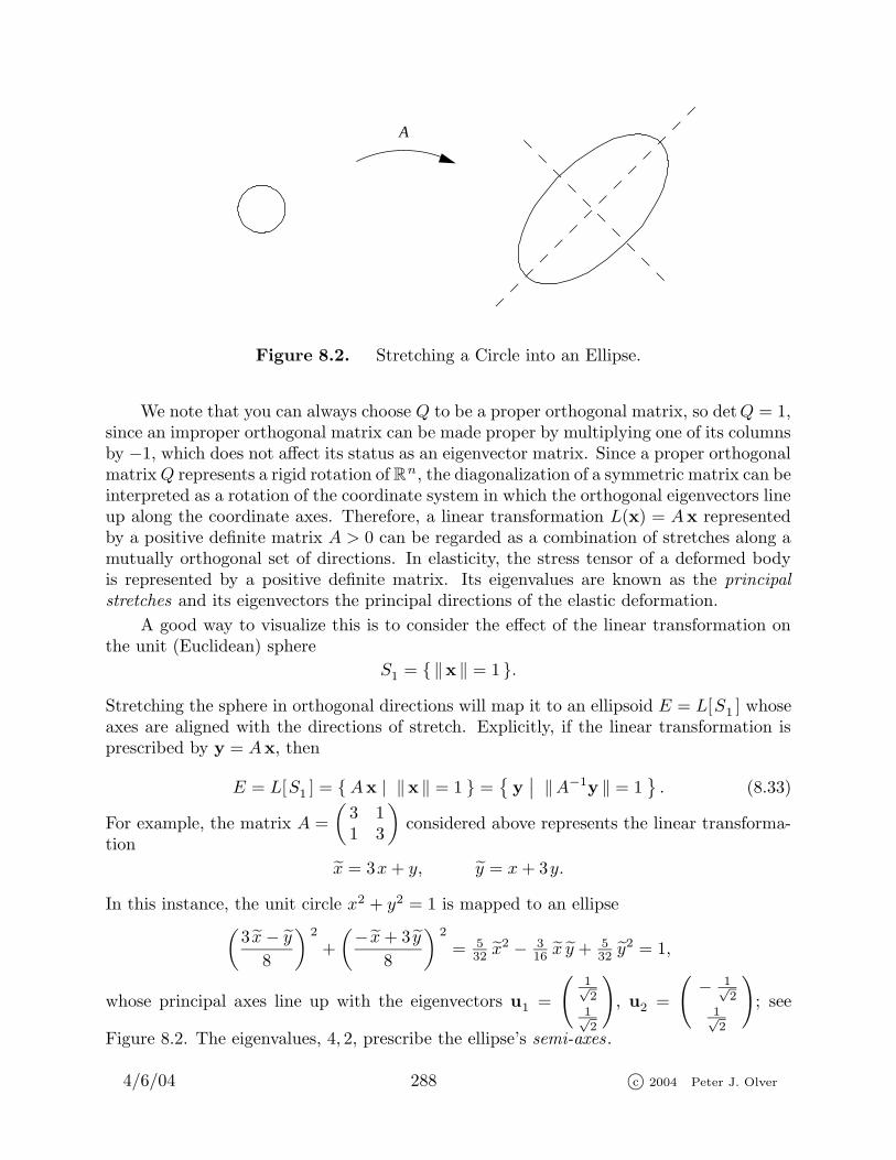
Figure 8.2. Stretching a Circle into an Ellipse.

We note that you can always choose Q to be a proper orthogonal matrix, so detQ = 1,since an improper orthogonal matrix can be made proper by multiplying one of its columnsby −1, which does not affect its status as an eigenvector matrix. Since a proper orthogonalmatrix Q represents a rigid rotation of R

n, the diagonalization of a symmetric matrix can beinterpreted as a rotation of the coordinate system in which the orthogonal eigenvectors lineup along the coordinate axes. Therefore, a linear transformation L(x) = Ax representedby a positive definite matrix A > 0 can be regarded as a combination of stretches along amutually orthogonal set of directions. In elasticity, the stress tensor of a deformed bodyis represented by a positive definite matrix. Its eigenvalues are known as the principal

stretches and its eigenvectors the principal directions of the elastic deformation.

A good way to visualize this is to consider the effect of the linear transformation onthe unit (Euclidean) sphere

S1 = { ‖x ‖ = 1 }.

Stretching the sphere in orthogonal directions will map it to an ellipsoid E = L[S1 ] whoseaxes are aligned with the directions of stretch. Explicitly, if the linear transformation isprescribed by y = Ax, then

E = L[S1 ] = { Ax | ‖x ‖ = 1 } ={

y∣∣ ‖A−1y ‖ = 1

}. (8.33)

For example, the matrix A =

(3 11 3

)considered above represents the linear transforma-

tion

x = 3x + y, y = x + 3y.

In this instance, the unit circle x2 + y2 = 1 is mapped to an ellipse(

3 x − y

8

)2

+

(− x + 3 y

8

)2

= 532 x2 − 3

16 x y + 532 y2 = 1,

whose principal axes line up with the eigenvectors u1 =

(1√2

1√2

), u2 =

(− 1√

2

1√2

); see

Figure 8.2. The eigenvalues, 4, 2, prescribe the ellipse’s semi-axes.

4/6/04 288 c© 2004 Peter J. Olver

Optimization Principles for Eigenvalues

As we learned in Chapter 4, the solution to a linear system with positive definitecoefficient matrix can be characterized by a minimization principle. Thus, it should come asno surprise that eigenvalues of positive definite, and even more general symmetric matrices,can also be characterized by some sort of optimization procedure. A number of basicnumerical algorithms for computing eigenvalues, of both matrices and, later on, differentialoperators are based on such optimization principles.

First consider the relatively simple case of a diagonal matrix Λ = diag (λ1, . . . , λn).We assume that the diagonal entries, which are the same as the eigenvalues, appear indecreasing order,

λ1 ≥ λ2 ≥ · · · ≥ λn, (8.34)

so λ1 is the largest eigenvalue, while λn is the smallest. The effect of Λ on a vector

y = ( y1, y2, . . . , yn )T ∈ R

n is to multiply its entries by the diagonal eigenvalues: Λy =

(λ1 y1, λ2 y2, . . . , λn yn )T. In other words, the linear transformation represented by the

coefficient matrix Λ has the effect of stretching† the ith coordinate direction by the factorλi. In particular, the maximal stretch occurs in the e1 direction, with factor λ1, while theminimal (or largest negative) stretch occurs in the en direction, with factor λn. The germof the optimization principles for characterizing the extreme eigenvalues is contained inthis geometrical observation.

Let us turn our attention to the associated quadratic form

q(y) = yT Λy = λ1 y21 + λ2 y2

2 + · · · + λn y2n. (8.35)

Note that q(t e1) = λ1 t2, and hence if λ1 > 0, then q(y) has no maximum; on the otherhand, if λ1 ≤ 0, so all eigenvalues are non-positive, then q(y) ≤ 0 for all y, and its maximalvalue is q(0) = 0. Thus, in either case, a strict maximization of q(y) is of no help.

Suppose, however, that we try to maximize q(y) but restrict y to be a unit vector (inthe Euclidean norm):

‖y ‖2 = y21 + · · · + y2

n = 1.

In view of (8.34),

q(y) = λ1 y21 +λ2 y2

2 + · · · +λn y2n ≤ λ1 y2

1 +λ1 y22 + · · · +λ1 y2

n = λ1

(y21 + · · · + y2

n

)= λ1.

Moreover, q(e1) = λ1. We conclude that the maximal value of q(y) over all unit vectors is

the largest eigenvalue of Λ:

λ1 = max { q(y) | ‖y ‖ = 1 } .

By the same reasoning, its minimal value equals the smallest eigenvalue:

λn = min { q(y) | ‖y ‖ = 1 }

† If λi < 0, then the effect is to stretch and reflect.

4/6/04 289 c© 2004 Peter J. Olver

Thus, we can characterize the two extreme eigenvalues by optimization principles, albeitof a slightly different character than we treated in Chapter 4.

Now suppose A is any symmetric matrix. We use the spectral decomposition (8.31)to diagonalize the associated quadratic form

q(x) = xT Ax = xT QΛQT x = yT Λy, where y = QT x = Q−1x,

as in (8.32). According to the preceding discussion, the maximum of yT Λy over all unitvectors ‖y ‖ = 1 is the largest eigenvalue λ1 of Λ, which is the same as the largesteigenvalue of A. Moreover, since Q is an orthogonal matrix, Proposition 7.24 tell us thatit maps unit vectors to unit vectors:

1 = ‖y ‖ = ‖QT x ‖ = ‖x ‖,

and so the maximum of q(x) over all unit vectors ‖x ‖ = 1 is the same maximum eigenvalueλ1. Similar reasoning applies to the smallest eigenvalue λn. In this fashion, we haveestablished the basic optimization principles for the extreme eigenvalues of a symmetricmatrix.

Theorem 8.27. If A is a symmetric matrix, then

λ1 = max{

xT Ax∣∣ ‖x ‖ = 1

}, λn = min

{xT Ax

∣∣ ‖x ‖ = 1}

, (8.36)

are, respectively its largest and smallest eigenvalues.

The maximal value is achieved when x = ±u1 is one of the unit eigenvectors corre-sponding to the largest eigenvalue; similarly, the minimal value is at x = ±un.

Remark : In multivariable calculus, the eigenvalue λ plays the role of a Lagrange mul-

tiplier for the constrained optimization problem. See [9] for details.

Example 8.28. The problem is to maximize the value of the quadratic form

q(x, y) = 3x2 + 2xy + 3y2

for all x, y lying on the unit circle x2 + y2 = 1. This maximization problem is precisely of

form (8.36). The coefficient matrix is A =

(3 11 3

), whose eigenvalues are, according to

Example 8.5, λ1 = 4 and λ2 = 2. Theorem 8.27 implies that the maximum is the largesteigenvalue, and hence equal to 4, while its minimum is the smallest eigenvalue, and henceequal to 2. Thus, evaluating q(x, y) on the unit eigenvectors, we conclude that

q(− 1√

2, 1√

2

)= 2 ≤ q(x, y) ≤ 4 = q

(− 1√

2, 1√

2

)for all x2 + y2 = 1.

In practical applications, the restriction of the quadratic form to unit vectors maynot be particularly convenient. One can, however, rephrase the eigenvalue optimizationprinciples in a form that utilizes general vectors. If v 6= 0 is any nonzero vector, thenx = v/‖v ‖ is a unit vector. Substituting this expression for x in the quadratic form

4/6/04 290 c© 2004 Peter J. Olver

q(x) = xT Ax leads to the following optimization principles for the extreme eigenvalues ofa symmetric matrix:

λ1 = max

{vT Av

‖v ‖2

∣∣∣∣ v 6= 0

}, λn = min

{vT Av

‖v ‖2

∣∣∣∣ v 6= 0

}. (8.37)

Thus, we replace optimization of a quadratic polynomial over the unit sphere by opti-mization of a rational function over all of R

n\{0}. Referring back to Example 8.28, themaximum value of

r(x, y) =3x2 + 2xy + 3y2

x2 + y2for all

(xy

)6=(

00

)

is equal to 4, the same maximal eigenvalue of the corresponding coefficient matrix.

What about characterizing one of the intermediate eigenvalues? Then we need tobe a little more sophisticated in designing the optimization principle. To motivate theconstruction, look first at the diagonal case. If we restrict the quadratic form (8.35) to

vectors y = ( 0, y2, . . . , yn )T

whose first component is zero, we obtain

q(y) = q(0, y2, . . . , yn) = λ2 y22 + · · · + λn y2

n.

The maximum value of q(y) over all such y of norm 1 is, by the same reasoning, the secondlargest eigenvalue λ2. Moreover, we can characterize such vectors geometrically by notingthat y · e1 = 0, and so they are orthogonal to the first standard basis vector, which alsohappens to be the eigenvector of Λ corresponding to the eigenvalue λ1. Similarly, if wewant to find the jth largest eigenvalue λj , we maximize q(y) over all unit vectors y whosefirst j−1 components vanish, y1 = · · · = yj−1 = 0, or, stated geometrically, over all vectorsy such that ‖ y ‖ = 1 and y · e1 = · · · = y · ej−1 = 0, i.e., over all vectors orthogonal tothe first j − 1 eigenvectors of Λ.

A similar reasoning based on the Spectral Theorem 8.25 and the orthogonality ofeigenvectors of symmetric matrices, leads to the general result.

Theorem 8.29. Let A be a symmetric matrix with eigenvalues λ1 ≥ λ2 ≥ · · · ≥λn and corresponding orthogonal eigenvectors v1, . . . ,vn. Then the maximal value of

the quadratic form xT Ax over all unit vectors which are orthogonal to the first j − 1eigenvectors is its jth eigenvalue:

λj = max{

xT Ax∣∣ ‖x ‖ = 1, x · v1 = · · · = x · vj−1 = 0

}. (8.38)

Thus, at least in principle, one can compute the eigenvalues and eigenvectors of asymmetric matrix by the following recursive procedure. First, find the largest eigenvalueλ1 by the basic maximization principle (8.36) and its associated eigenvector v1 by solvingthe eigenvector system (8.13). The next largest eigenvalue λ2 is then characterized by theconstrained minimization principle (8.38), and so on. Although of theoretical interest, thisalgorithm is not effective in practical numerical computations.

4/6/04 291 c© 2004 Peter J. Olver

8.5. Singular Values.

We have already indicated the central role played by the eigenvalues and eigenvectorsof a square matrix in both theory and applications. Much more evidence to this effectwill appear in the ensuing chapters. Alas, non-square matrices do not have eigenvalues(why?), and so, at first glance, do not appear to possess any quantities of comparablesignificance. However, our earlier treatment of least squares minimization problems aswell as the equilibrium equations for structures and circuits made essential use of thesymmetric, positive semi-definite square Gram matrix K = AT A — which can be naturallyformed even when A is rectangular. Perhaps the eigenvalues of K might play a comparablyimportant role for general matrices. Since they are not easily related to the eigenvalues ofA — which, in the truly rectangular case, don’t even exist — we shall endow them with anew name.

Definition 8.30. The singular values σ1, . . . , σn of an m × n matrix A are thesquare roots, σi =

√λi , of the eigenvalues of the associated Gram matrix K = AT A. The

corresponding eigenvectors of K are known as the singular vectors of A.

Since K is necessarily positive semi-definite, its eigenvalues are always non-negative,λi ≥ 0, and hence the singular values of A are also all non-negative†, σi ≥ 0 — no matterwhether A itself has positive, negative, or even complex eigenvalues, or is rectangular andhas no eigenvalues at all. However, for symmetric matrices, there is a direct connectionbetween the two quantities:

Proposition 8.31. If A = AT is a symmetric matrix, its singular values are the ab-

solute values of its eigenvalues: σi = |λi |; its singular vectors coincide with the associated

eigenvectors.

Proof : When A is symmetric, K = AT A = A2. So, if Av = λv, then Kv = A2v =λ2v. Thus, every eigenvector v of A is also an eigenvector of K with eigenvalue λ2.Therefore, the eigenvector basis of A is an eigenvector basis for K, and hence forms acomplete system of singular vectors for A also. Q.E.D.

The standard convention is to label the singular values in decreasing order, so thatσ1 ≥ σ2 ≥ · · · ≥ σn ≥ 0. Thus, σ1 will always denote the largest or dominant singularvalue. If AT A has repeated eigenvalues, the singular values of A are repeated with thesame multiplicities.

Example 8.32. Let A =

(3 54 0

). The associated Gram matrix is K = AT A =

(25 1515 25

), with eigenvalues λ1 = 40 and λ2 = 10. Thus, the singular values of A are

σ1 =√

40 ≈ 6.3246 . . . and σ2 =√

10 ≈ 3.1623 . . . . Note that these are not the same asits eigenvalues, namely λ1 = 1

2 (3 +√

89) ≈ 6.2170 . . . , λ2 = 12 (3 −

√89) ≈ −3.2170.

† Warning : Some authors, e.g., [123], only designate the nonzero σi’s as singular values.

4/6/04 292 c© 2004 Peter J. Olver

A rectangular matrix Σ will be called diagonal if its only nonzero entries are on themain diagonal starting in the upper left hand corner, and so σij = 0 for i 6= j. An exampleis the matrix

Σ =

5 0 0 00 3 0 00 0 0 0

whose only nonzero entries are in the diagonal (1, 1) and (2, 2) positions. (Its last diagonalentry happens to be 0.)

The generalization of the spectral factorization to non-symmetric matrices is knownas the singular value decomposition, commonly abbreviated as SVD. Unlike the spectraldecomposition, the singular value decomposition applies to arbitrary real rectangular ma-trices.

Theorem 8.33. Any real m × n matrix A can be factorized

A = P ΣQT (8.39)

into the product of an m × m orthogonal matrix P , the m × n diagonal matrix Σ that

has the first l = min{m,n} singular values of A as its diagonal entries, and an n × northogonal matrix QT .

Proof : Writing the factorization (8.39) as AQ = P Σ, and looking at the columns ofthe resulting matrix equation, we are led to the vector equations

Aui = σi vi, i = 1, . . . , n, (8.40)

relating the orthonormal columns of Q = (u1 u2 . . . un ) to the orthonormal columns ofP = (v1 v2 . . . vm ). The scalars σi in (8.40) are the diagonal entries of Σ or, if m < i ≤ n,equal to 0. The fact that P and Q are both orthogonal matrices means that their columnvectors form orthonormal bases for, respectively, R

m and Rn under the Euclidean dot

product. In this manner, the singular values indicate how far the linear transformationrepresented by the matrix A stretches a distinguished set of orthonormal basis vectors.

To construct the required bases, we prescribe u1, . . . ,un to be the orthonormal eigen-vector basis of the Gram matrix K = AT A; thus

AT Auj = Kuj = λj uj = σ2j uj .

We claim that the image vectors wi = Aui are automatically orthogonal. Indeed, in viewof the orthonormality of the ui,

wi · wj = wTi wj = (Aui)

T Auj = uTi AT Auj = σ2

j uTi uj = σ2

j ui · uj =

{0, i 6= j,

σ2i , i = j.

.

(8.41)Consequently, w1, . . . ,wn form an orthogonal system of vectors having respective norms

‖wi ‖ =√

wi · wi = σi.

Since u1, . . . ,un form a basis of Rn, their images w1 = Au1, . . . ,wn = Aun span

rng A. Suppose that A has r non-zero singular values, so σr+1 = · · · = σn = 0. Then

4/6/04 293 c© 2004 Peter J. Olver

the corresponding image vectors w1, . . . ,wr are non-zero, mutually orthogonal vectors,and hence form an orthogonal basis for rng A. Since the dimension of rng A is equal toits rank, this implies that the number of non-zero singular values is r = rank A. Thecorresponding unit vectors

vi =wi

σi

=Aui

σi

, i = 1, . . . , r, (8.42)

are an orthonormal basis for rng A. Let us further select an orthonormal basis vr+1, . . . ,vm

for its orthogonal complement coker A = (rng A)⊥. The combined set of vectors v1, . . . ,vm

clearly forms an orthonormal basis of Rm, and satisfies (8.40) as required. In this manner,

the resulting orthonormal bases u1, . . . ,un and v1, . . . ,vm form the respective columns ofthe orthogonal matrices Q,P in the singular value decomposition (8.39). Q.E.D.

Warning : If m < n, then only the first m singular values appear along the diagonalof Σ. It follows from the proof that the remaining n − m singular values are all zero.

Example 8.34. For the matrix A =

(3 54 0

)considered in Example 8.32, the

orthonormal eigenvector basis of K = AT A =

(25 1515 25

)is given by the unit singular

vectors u1 =

(1√2

1√2

)and u2 =

(− 1√

2

1√2

). Thus, Q =

(1√2

− 1√2

1√2

1√2

). On the other hand,

according to (8.42),

v1 =Au1

σ1

=1√40

(4√

2

2√

2

)=

(2√5

1√5

), v2 =

Au2

σ2

=1√10

( √2

− 2√

2

)=

(1√5

− 2√5

),

and thus P =

(2√5

1√5

1√5

− 2√5

). You may wish to validate the resulting singular value

decomposition

A =

(3 54 0

)=

(2√5

1√5

1√5

− 2√5

) (√40 0

0√

10

) (1√2

1√2

− 1√2

1√2

)= P ΣQT .

As their name suggests, the singular values can be used to detect singular matrices.Indeed, the singular value decomposition tells us some interesting new geometrical infor-mation about matrix multiplication, supplying additional details to the discussion begunin Section 2.5 and continued in Section 5.6. The next result follows directly from the proofof Theorem 8.33.

Theorem 8.35. Let σ1, . . . , σr > 0 be the non-zero singular values of the m × nmatrix A. Let v1, . . . ,vm and u1, . . . ,un be the orthonormal bases of, respectively, R

m and

Rn provided by the columns of P and Q in its singular value decomposition A = P ΣQT .

Then (i) r = rank A,

4/6/04 294 c© 2004 Peter J. Olver

(ii) u1, . . . ,ur form an orthonormal basis for corng A,

(iii) ur+1, . . . ,un form an orthonormal basis for ker A,

(iv) v1, . . . ,vr form an orthonormal basis for rng A,

(v) vr+1, . . . ,vm form an orthonormal basis for coker A.

We already noted in Section 5.6 that the linear transformation L: Rn → Rm defined by

matrix multiplication, L[x ] = Ax, can be interpreted as a projection from Rn to corng A

followed by an invertible map from corng A to rng A. The singular value decompostiontells us that not only is the latter map invertible, it is simply a combination of stretchesin the r mutually orthogonal singular directions u1, . . . ,ur, whose magnitudes equal thenonzero singular values. In this way, we have at last reached a complete understanding ofthe subtle geometry underlying the simple operation of matrix multiplication.

An alternative interpretation of the singular value decomposition is to view the twoorthogonal matrices in (8.39) as defining rigid rotations/reflections. Therefore, in all cases,a linear transformation from R

n to Rm is composed of three ingredients:

(i) A rotation/reflection of the domain space Rn, as prescribed by QT , followed by

(ii) a simple stretching map of the coordinate vectors e1, . . . , en of domain space, map-ping ei to σi ei in the target space R

m, followed by

(iii) a rotation/reflection of the target space, as prescribed by P .

In fact, in most cases we can choose both P and Q to be proper orthogonal matricesrepresenting rotations; see Exercise .

Condition Number, Rank, and Principal Component Analysis

The singular values not only provide a nice geometric interpretation of the action ofthe matrix, they also play a key role in modern computational algorithms. The relativemagnitudes of the singular values can be used to distinguish well-behaved linear systemsfrom ill-conditioned systems which are much trickier to solve accurately. Since the numberof nonzero singular values equals its rank, a square matrix that has one or more zerosingular values is singular. A matrix with one or more very small singular values shouldbe considered to be close to singular. Such ill-conditioning is traditionally quantified asfollows.

Definition 8.36. The condition number of an n × n matrix is the ratio between itslargest and smallest singular value: κ(A) = σ1/σn.

A matrix with a very large condition number is said to be ill-conditioned ; in practice,this occurs when the condition number is larger than the reciprocal of the machine’sprecision, e.g., 106 for most single precision arithmetic. As the name implies, it is muchharder to solve a linear system Ax = b when its coefficient matrix is ill-conditioned. Inthe extreme case when A has one or more zero singular values, so σn = 0, its conditionnumber is infinite, and the linear system is singular, with either no solution or infinitelymany solutions.

The accurate computation of the rank of a matrix can be a numerical challenge. Small

numerical errors in the entries can have a dramatic effect. For example, A =

1 1 −12 2 −23 3 −3

4/6/04 295 c© 2004 Peter J. Olver

has rank r = 1, but a tiny change, say to A =

1.00001 1 −12 2.00001 −23 3 −3.00001

, will

produce a nonsingular matrix with rank r = 3. The latter matrix, however, is very closeto singular, and this is highlighted by their respective singular values. For the first matrix,they are σ1 =

√42 ≈ 6.48 and σ2 = σ3 = 0, reconfirming that A has rank 1, whereas for

A we find σ1 ≈ 6.48075 while σ2 ≈ σ3 ≈ .000001. The fact that the second and third

singular values are very small indicates that A is very close to a matrix of rank 1 andshould be viewed as a numerical or experimental perturbation of such a matrix. Thus,the most effective practical method for computing the rank of a matrix is to first assigna threshhold, e.g., 10−5, for singular values, and then treat any small singular value lyingbelow the threshold as if it were zero.

This idea underlies the method of Principal Component Analysis that is playing anincreasingly visible role in modern statistics, data analysis and data mining, imaging,and a variety of other fields, [89]. The singular vectors associated with the larger singularvalues indicate the principal components of the matrix, while small singular values indicateunimportant directions. In applications, the columns of the matrix A represent the datavectors, which are normalized to have mean 0. The corresponding Gram matrix K = AT Acan be identified as the associated covariance matrix . Its eigenvectors are the principalcomponents that serve indicate directions of correlation and clustering to be found inthe data. Classification of patterns in images, sounds, semantics, and so on are beingsuccessfully handled by this powerful new approach.

The Pseudoinverse

With the singular value decomposition in hand, we are able to introduce a general-ization of the inverse that applies to cases when the matrix in question is singular or evenrectangular. We begin with the diagonal case. Let Σ be an m × n diagonal matrix withr nonzero diagonal entries σ1, . . . , σr. We define the pseudoinverse of Σ to be the n × mdiagonal matrix Σ+ whose nonzero diagonal entries are the reciprocals 1/σ1, . . . , 1/σr. Forexample, if

Σ =

5 0 0 00 3 0 00 0 0 0

, then Σ+ =

15 0 00 1

3 00 0 00 0 0

.

The zero diagonal entries are not inverted. In particular, if Σ is a nonsingular squarediagonal matrix, then its pseudoinverse and ordinary inverse are the same: Σ+ = Σ−1.

Definition 8.37. The pseudoinverse of an m × n matrix A with singular valuedecomposition A = P ΣQT is the n × m matrix A+ = QΣ+ PT .

Note that the latter equation is the singular value decomposition of the pseudoinverseA+, and hence its nonzero singular values are the reciprocals of the nonzero singular valuesof A. If A is a non-singular square matrix, then its pseudoinverse agrees with its ordinary

4/6/04 296 c© 2004 Peter J. Olver

inverse, since

A−1 = (P ΣQT )−1 = (Q−1)T Σ−1 P−1 = QΣ+ PT = A+,

where we used the fact that the inverse of an orthogonal matrix is equal to its transpose.

If A is square and nonsingular, then, as we know, the solution to the linear systemAx = b is given by x? = A−1b. For a general coefficient matrix, the vector x? = A+b

obtained by applying the pseudoinverse to the right hand side plays a distinguished role— it is the least squares soution to the system! In this manner, the pseudoinverse providesus with a direct route to least squares solutions to systems of linear equations.

Theorem 8.38. Consider the linear system Ax = b. Let x? = A+b, where A+ is

the pseudoinverse of A. If ker A = {0}, then x? ∈ corng A is the least squares solution to

the system. If, more generally, ker A 6= {0}, then x? is the least squares solution of minimal

Euclidean norm among all vectors that minimize the least squares error ‖Ax − b ‖.Proof : To show that x? = A+b is the least squares solution to the system, we must

check that it satisfies the normal equations AT Ax? = AT b. Using the definition of thepseudoinverse and the singular value decomposition (8.39), we find

AT Ax? = AT AA+b = (P ΣQT )T (P ΣQT )(QΣ+PT )b

= QΣT ΣΣ+PT b = QΣT PT b = AT b,

where the next to last equality is left as Exercise for the reader. This proves that x?

solves the normal equations, and hence minimizes the least squares error†.

Thus, when rank A = n, the vector x? is the unique least squares aolution to thesystem. More generally, if A has rank r < n, so, ker A 6= {0}, only the first r singularvalues are nonzero, and therefore the last n− r rows of Σ+ are all zero. This implies thatthe last n−r entries of the vector c = Σ+PT b are also all zero, so c = ( c1, . . . cr, 0, . . . , 0 )

T.

We conclude that

x? = A+b = QΣ+ PT b = Qc = c1u1 + · · · + cr ur

is a linear combination of the first r singular vectors, and hence, by Theorem 8.35, x? ∈corng A. The most general least squares solution has the form x = x? +z where z ∈ ker A,and the fact that ‖x? ‖ is minimized follows as in Theorem 5.57. Q.E.D.

When forming the pseudoinverse, we see see that very small singular values lead to verylarge entries in Σ+, which will cause numerical difficulties when computing the least squaressolution x? = A+b to the linear system. A common and effective computational strategyto avoid the effects of small singular values is to replace the corresponding diagonal entriesof the pseudoinverse Σ+ by 0. This has the effect of regularizing ill-conditioned matricesthat are very close to singular — rather than solve the system directly for x = A−1b, onewould employ the suitably regularized pseudoinverse.

Finally, we note that practical numerical algorithms for computing singular valuesand the singular value decomposition can be found in [68, 123]

† In Chapter 4, this was proved under the assumption that ker A = {0}. You are asked toestablish the general case in Exercise .

4/6/04 297 c© 2004 Peter J. Olver

8.6. Incomplete Matrices and the Jordan Canonical Form.

Unfortunately, not all matrices are complete. Matrices that do not have enough (com-plex) eigenvectors to form a basis are considerably less pleasant to work with. However, asthey occasionally appear in applications, it is worth learning how to handle them. We shallshow how to supplement the eigenvectors in order to obtain a basis in which the matrixassumes a simple, but now non-diagonal form. The resulting construction is named afterthe nineteenth century French mathematician Camille Jordan‡.

Throughout this section, A will be an n × n matrix, with either real or complexentries. We let λ1, . . . , λk denote the distinct eigenvalues of A. We recall that Theorem 8.10guarantees that every matrix has at least one (complex) eigenvalue, so k ≥ 1. Moreover,we are assuming that k < n, as otherwise A would be complete.

Definition 8.39. A Jordan chain of length j is a sequence of non-zero vectorsw1, . . . ,wj ∈ C

m that satisfies

Aw1 = λw1, Awi = λwi + wi−1, i = 2, . . . , j, (8.43)

where λ is an eigenvalue of A.

Note that the initial vector w1 in a Jordan chain is a genuine eigenvector, and soJordan chains only exist when λ is an eigenvalue. The other vectors, w2, . . . ,wj , aregeneralized eigenvectors, in accordance with the following definition.

Definition 8.40. A nonzero vector w 6= 0 that satisfies

(A − λ I )k w = 0 (8.44)

for some k > 0 and λ ∈ C is called a generalized eigenvector of the matrix A.

Note that every ordinary eigenvector is automatically a generalized eigenvector, sincewe can just take k = 1 in (8.44); the converse is not necessarily valid. We shall call theminimal value of k for which (8.44) holds the index of the generalized eigenvector. Thus,an ordinary eigenvector is a generalized eigenvector of index 1. Since A−λ I is nonsingularwhenever λ is not an eigenvalue of A, its kth power (A−λ I )k is also nonsingular. Therefore,generalized eigenvectors can only exist when λ is an ordinary eigenvalue of A — there areno additional “generalized eigenvalues”.

Lemma 8.41. The ith vector wi in a Jordan chain (8.43) is a generalized eigenvector

of index i.

Proof : By definition, (A − λ I )w1 = 0, and so w1 is an eigenvector. Next, we have(A − λ I )w2 = w1, and so (A − λ I )2w2 = (A − λ I )w1 = 0. Thus, w2 a generalizedeigenvector of index 2. A simple induction proves that (A − λ I )i wi = 0. Q.E.D.

‡ No relation to Wilhelm Jordan of Gauss–Jordan fame.

4/6/04 298 c© 2004 Peter J. Olver

Example 8.42. Consider the 3× 3 Jordan block A =

2 1 00 2 10 0 2

. The only eigen-

value is λ = 2, and A − 2 I =

0 1 00 0 10 0 0

. We claim that the standard basis vectors

e1, e2 and e3 form a Jordan chain. Indeed, Ae1 = 2e1, and hence e1 ∈ ker(A − 2 I ) isa genuine eigenvector. Furthermore, Ae2 = 2e2 + e1, and Ae3 = 2e3 + e2, as you caneasily check. Thus, e1, e2 and e3 satisfy the Jordan chain equations for the eigenvalue

λ = 2. Note that e2 lies in the kernel of (A− 2 I )2 =

0 0 10 0 00 0 0

, and so is a generalized

eigenvector of index 2. Indeed, every vector of the form w = ae1 + be2 with b 6= 0 is ageneralized eigenvector of index 2. (When b = 0, a 6= 0, the vector w = ae1 is an ordinaryeigenvector of index 1.) Finally, (A− 2 I )3 = O, and so every vector v ∈ R

3, including e3,is a generalized eigenvector of index 3 (or less).

A basis of Rn or C

n is called a Jordan basis for the matrix A if it consists of one ormore Jordan chains that have no elements in common. Thus, for the Jordan matrix inExample 8.42, the standard basis e1, e2, e3 is, in fact, a Jordan basis. An eigenvector basisqualifies as a Jordan basis, since each eigenvector belongs to a Jordan chain of length 1.Jordan bases are the desired extension of eigenvector bases, and every square matrix hasone.

Theorem 8.43. Every n×n matrix admits a Jordan basis of Cn. The first elements

of the Jordan chains form a maximal system of linearly independent eigenvectors. More-

over, the number of generalized eigenvectors in the Jordan basis that belong to the Jordan

chains associated with the eigenvalue λ is the same as the eigenvalue’s multiplicity.

Example 8.44. Consider the matrix

A =

−1 0 1 0 0−2 2 −4 1 1−1 0 −3 0 0−4 −1 3 1 04 0 2 −1 0

.

With some work, its characteristic equation is found to be

pA(λ) = det(A − λ I ) = λ5 + λ4 − 5λ3 − λ2 + 8λ − 4 = (λ − 1)3(λ + 2)2 = 0,

and hence A has two eigenvalues: λ1 = 1, which is a triple eigenvalue, and λ2 = −2, whichis double. Solving the associated homogeneous systems (A−λj I )v = 0, we discover that,

up to constant multiple, there are only two eigenvectors: v1 = ( 0, 0, 0,−1, 1 )T

for λ1 = 1

and, anticipating our final numbering, v4 = (−1, 1, 1,−2, 0 )T

for λ2 = −2. Thus, A is farfrom complete.

To construct a Jordan basis, we first note that since A has 2 linearly independenteigenvectors, the Jordan basis will contain two Jordan chains; the one associated with the

4/6/04 299 c© 2004 Peter J. Olver

triple eigenvalue λ1 = 1 has length 3, while λ2 = −2 admits a Jordan chain of length2. To construct the former, we need to first solve the system (A − I )w = v1. Notethat the coefficient matrix is singular — it must be since 1 is an eigenvalue — and thegeneral solution is w = v2+tv1 where v2 = ( 0, 1, 0, 0,−1 )

T, and t is the free variable. The

appearance of an arbitrary multiple of the eigenvector v1 in the solution is not unexpected;indeed, the kernel of A− I is the eigenspace for λ1 = 1. We can choose any solution, e.g.,v2 as the second element in the Jordan chain. To find the last element of the chain, we

solve (A − I )w = v2 to find w = v3 + tv1 where v3 = ( 0, 0, 0, 1, 0 )T

can be used as thelast element of this Jordan chain. Similarly, to construct the Jordan chain for the secondeigenvalue, we solve (A+2 I )w = v4 and find w = v5 + tv4 where v5 = (−1, 0, 0,−2, 1 )

T.

Thus, the desired Jordan basis is

v1 =

000−11

, v2 =

0100−1

, v3 =

00010

, v4 =

−111−20

, v5 =

−100−21

,

with Av1 = v1, Av2 = v1 + v2, Av3 = v2 + v2, Av4 = −2v4, Av5 = v4 − 2v5.

To prove Theorem 8.43, we begin with a simple lemma.

Lemma 8.45. If v1, . . . ,vn forms a Jordan basis for the matrix A, it also forms a

Jordan basis for B = A − c I , for any scalar c.

Proof : We note that the eigenvalues of B are of the form λ−c, where λ is an eigenvalueof A. Moreover, given a Jordan chain w1, . . . ,wj of A, we have

Bw1 = (λ − c)w1, Bwi = (λ − c)wi + wi−1, i = 2, . . . , j,

so w1, . . . ,wj is also a Jordan chain for B corresponding to the eigenvalue λ − c. Q.E.D.

The proof of Theorem 8.43 will be done by induction on the size n of the matrix. Thecase n = 1 is trivial, since any nonzero element of C is a Jordan basis for a 1 × 1 matrixA = (a). To perform the induction step, we assume that the result is valid for all matricesof size ≤ n− 1. Let A be an n×n matrix. According to Theorem 8.10, A has at least onecomplex eigenvalue λ. Let B = A − λ I . Since λ is an eigenvalue of A, we know that 0 isan eigenvalue of B. This means that ker B 6= {0}, and so r = rank B < n. Moreover, byLemma 8.45, any Jordan basis of B is also a Jordan basis for A, and so we can concentrateall our attention on the singular matrix B from now on.

We note that W = rng B ⊂ Cn is an invariant subspace, i.e., Bw ∈ W whenever

w ∈ W , cf. Exercise . Moreover, since B is singular, dim W = r = rank B < n. Thus, byfixing a basis of W , we can realize the restriction B:W → W as multiplication by an r× rmatrix. The fact that r < n allows us to invoke the induction hypothesis, and deduce theexistence of a Jordan basis w1, . . . ,wr ∈ W ⊂ C

n for the action of B on the subspace W .Our goal is to complete this collection to a full Jordan basis on C

n.

To this end, we append two additional kinds of vectors. Suppose that the Jordan basisof W contains k null Jordan chains associated with its zero eigenvalue. Each null Jordan

4/6/04 300 c© 2004 Peter J. Olver

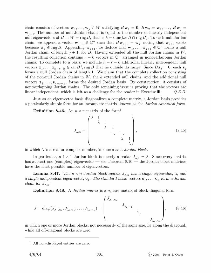
chain consists of vectors w1, . . . ,wj ∈ W satisfying Bw1 = 0, Bw2 = w1, . . . , Bwj =wj−1. The number of null Jordan chains is equal to the number of linearly independentnull eigenvectors of B in W = rng B, that is k = dim(ker B ∩ rng B). To each null Jordanchain, we append a vector wj+1 ∈ C

n such that Bwj+1 = wj , noting that wj+1 existsbecause wj ∈ rng B. Appending wj+1, we deduce that w1, . . . ,wj+1 ∈ C

n forms a nullJordan chain, of length j + 1, for B. Having extended all the null Jordan chains in W ,the resulting collection contains r + k vectors in C

n arranged in nonoverlapping Jordanchains. To complete to a basis, we include n − r − k additional linearly independent nullvectors z1, . . . , zn−r−k ∈ ker B \ rng B that lie outside its range. Since B zj = 0, each zj

forms a null Jordan chain of length 1. We claim that the complete collection consistingof the non-null Jordan chains in W , the k extended null chains, and the additional nullvectors z1, . . . , zn−r−k, forms the desired Jordan basis. By construction, it consists ofnonoverlapping Jordan chains. The only remaining issue is proving that the vectors arelinear independent, which is left as a challenge for the reader in Exercise . Q.E.D.

Just as an eigenvector basis diagonalizes a complete matrix, a Jordan basis providesa particularly simple form for an incomplete matrix, known as the Jordan canonical form.

Definition 8.46. An n × n matrix of the form†

Jλ,n =

λ 1λ 1

λ 1. . .

. . .

λ 1λ

, (8.45)

in which λ is a real or complex number, is known as a Jordan block .

In particular, a 1 × 1 Jordan block is merely a scalar Jλ,1 = λ. Since every matrixhas at least one (complex) eigenvector — see Theorem 8.10 — the Jordan block matriceshave the least possible number of eigenvectors.

Lemma 8.47. The n × n Jordan block matrix Jλ,n has a single eigenvalue, λ, and

a single independent eigenvector, e1. The standard basis vectors e1, . . . , en form a Jordan

chain for Jλ,n.

Definition 8.48. A Jordan matrix is a square matrix of block diagonal form

J = diag (Jλ1,n1, Jλ2,n2

, . . . , Jλk,nk) =

Jλ1,n1

Jλ2,n2

. . .

Jλk,nk

, (8.46)

in which one or more Jordan blocks, not necessarily of the same size, lie along the diagonal,while all off-diagonal blocks are zero.

† All non-displayed entries are zero.

4/6/04 301 c© 2004 Peter J. Olver

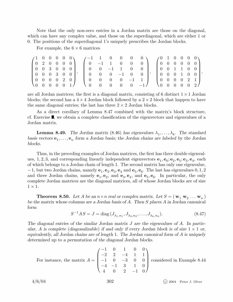
Note that the only non-zero entries in a Jordan matrix are those on the diagonal,which can have any complex value, and those on the superdiagonal, which are either 1 or0. The positions of the superdiagonal 1’s uniquely prescribes the Jordan blocks.

For example, the 6 × 6 matrices

1 0 0 0 0 00 2 0 0 0 00 0 3 0 0 00 0 0 3 0 00 0 0 0 2 00 0 0 0 0 1

,

−1 1 0 0 0 00 −1 1 0 0 00 0 −1 1 0 00 0 0 −1 0 00 0 0 0 −1 10 0 0 0 0 −1

,

0 1 0 0 0 00 0 0 0 0 00 0 1 1 0 00 0 0 1 0 00 0 0 0 2 10 0 0 0 0 2

,

are all Jordan matrices; the first is a diagonal matrix, consisting of 6 distinct 1× 1 Jordanblocks; the second has a 4× 4 Jordan block followed by a 2× 2 block that happen to havethe same diagonal entries; the last has three 2 × 2 Jordan blocks.

As a direct corollary of Lemma 8.47 combined with the matrix’s block structure,cf. Exercise , we obtain a complete classification of the eigenvectors and eigenvalues of aJordan matrix.

Lemma 8.49. The Jordan matrix (8.46) has eigenvalues λ1, . . . , λk. The standard

basis vectors e1, . . . , en form a Jordan basis; the Jordan chains are labeled by the Jordan

blocks.

Thus, in the preceding examples of Jordan matrices, the first has three double eigenval-ues, 1, 2, 3, and corresponding linearly independent eigenvectors e1, e6; e2, e5; e3, e4, eachof which belongs to a Jordan chain of length 1. The second matrix has only one eigenvalue,−1, but two Jordan chains, namely e1, e2, e3, e4 and e5, e6. The last has eigenvalues 0, 1, 2and three Jordan chains, namely e1, e2, and e3, e4, and e5, e6. In particular, the onlycomplete Jordan matrices are the diagonal matrices, all of whose Jordan blocks are of size1 × 1.

Theorem 8.50. Let A be an n×n real or complex matrix. Let S = (w1 w2 . . . wn )be the matrix whose columns are a Jordan basis of A. Then S places A in Jordan canonicalform

S−1AS = J = diag (Jλ1,n1, Jλ2,n2

, . . . , Jλk,nk). (8.47)

The diagonal entries of the similar Jordan matrix J are the eigenvalues of A. In partic-

ular, A is complete (diagonalizable) if and only if every Jordan block is of size 1 × 1 or,

equivalently, all Jordan chains are of length 1. The Jordan canonical form of A is uniquely

determined up to a permutation of the diagonal Jordan blocks.

For instance, the matrix A =

−1 0 1 0 0−2 2 −4 1 1−1 0 −3 0 0−4 −1 3 1 04 0 2 −1 0

considered in Example 8.44

4/6/04 302 c© 2004 Peter J. Olver

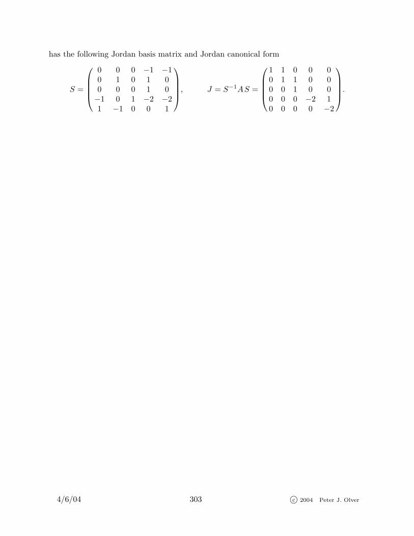
has the following Jordan basis matrix and Jordan canonical form

S =

0 0 0 −1 −10 1 0 1 00 0 0 1 0−1 0 1 −2 −21 −1 0 0 1

, J = S−1AS =

1 1 0 0 00 1 1 0 00 0 1 0 00 0 0 −2 10 0 0 0 −2

.

4/6/04 303 c© 2004 Peter J. Olver