Chapter 8: Long-Term Dynamics or Equilibrium 1.(8.1) Equilibrium 2.(8.2) Eigenvectors 3.(8.3) Stability 1.(8.1) Equilibrium 2.(8.2) Eigenvectors 3.(8.3)

Chapter 8: Long-Term Dynamics or Equilibrium

1. (8.1) Equilibrium2. (8.2) Eigenvectors3. (8.3) Stability

Notion of a Long-Term Equilibrium State

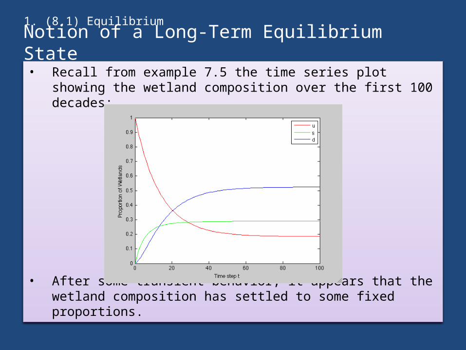
• Recall from example 7.5 the time series plot showing the wetland composition over the first 100 decades:

• After some transient behavior, it appears that the wetland composition has settled to some fixed proportions.

1. (8.1) Equilibrium


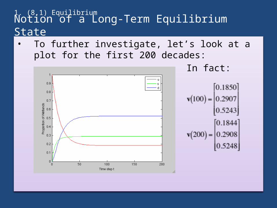
• To further investigate, let’s look at a plot for the first 200 decades:

In fact:



• We see that each class of the system approaches some fixed fraction/proportion

• What we want to do now is define a mathematical method to find this long-term state– It turns out that this long-term steady state is represented by an

eigenvector of the transfer matrix– In the models presented in this chapter**, the eigenvector is a

vector whose elements tell us what fraction of the system each class will have (well, the fraction that each class will approach) after a long time. This is also called the long-term equilibrium (or steady) state of the system.

– (**) Recall that the matrices we are working with right now all have a special form- they are transfer matrices; we will soon see that this particular definition for eigenvector applies only to this special case and will need to be generalized


Motivating Example

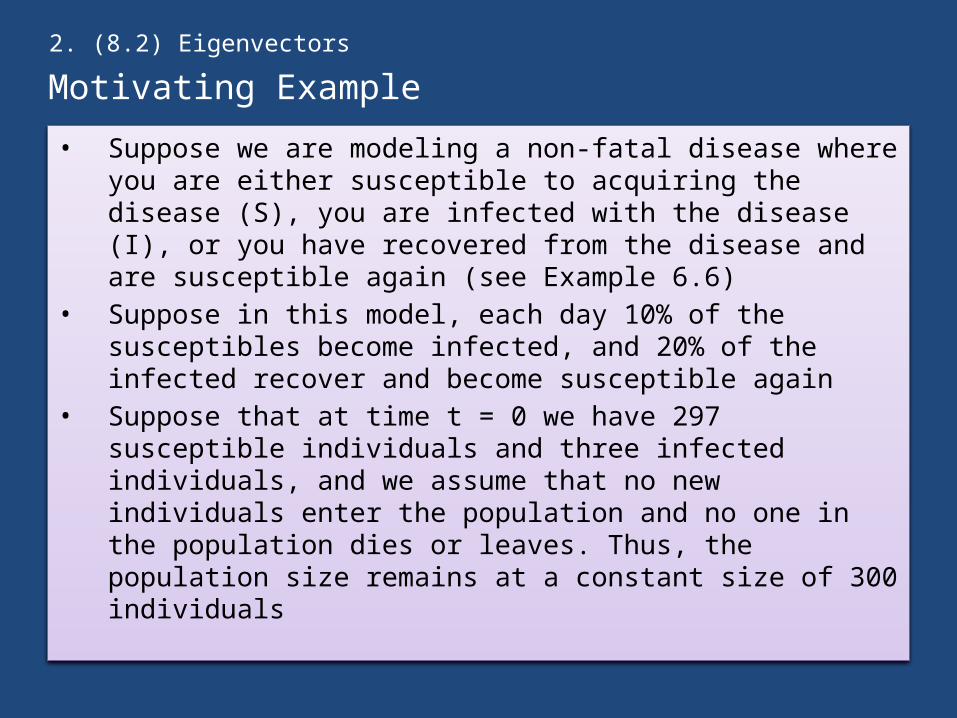
• Suppose we are modeling a non-fatal disease where you are either susceptible to acquiring the disease (S), you are infected with the disease (I), or you have recovered from the disease and are susceptible again (see Example 6.6)

• Suppose in this model, each day 10% of the susceptibles become infected, and 20% of the infected recover and become susceptible again

• Suppose that at time t = 0 we have 297 susceptible individuals and three infected individuals, and we assume that no new individuals enter the population and no one in the population dies or leaves. Thus, the population size remains at a constant size of 300 individuals

2. (8.2) Eigenvectors

Motivating Example

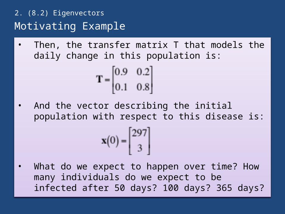
• Then, the transfer matrix T that models the daily change in this population is:

• And the vector describing the initial population with respect to this disease is:

• What do we expect to happen over time? How many individuals do we expect to be infected after 50 days? 100 days? 365 days?


Motivating Example

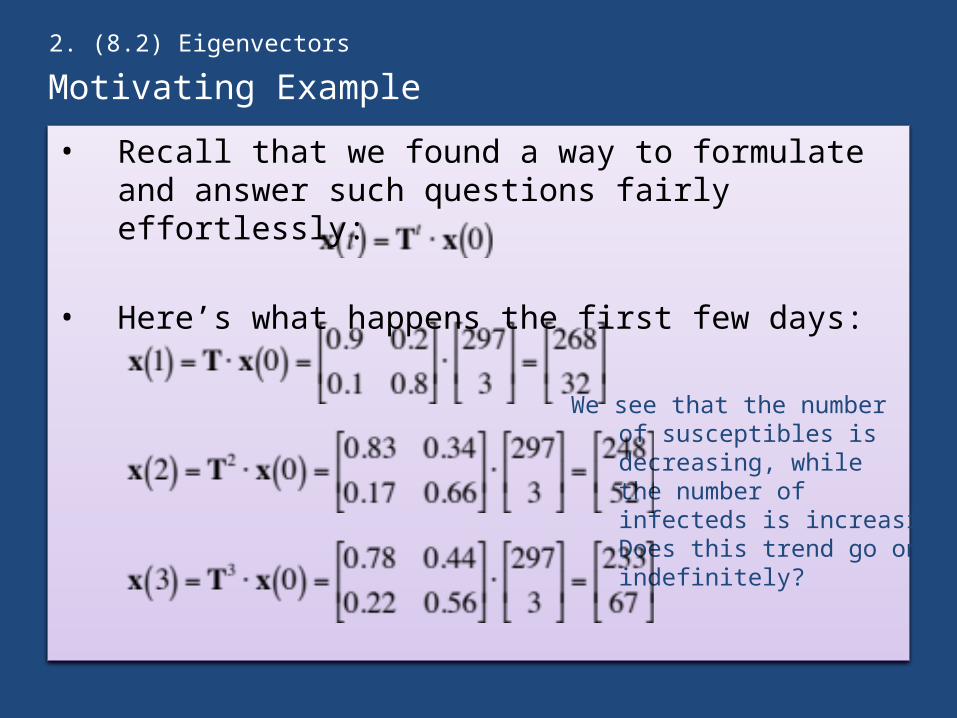
• Recall that we found a way to formulate and answer such questions fairly effortlessly:

• Here’s what happens the first few days:


We see that the numberof susceptibles isdecreasing, whilethe number ofinfecteds is increasing.Does this trend go onindefinitely?

Motivating Example

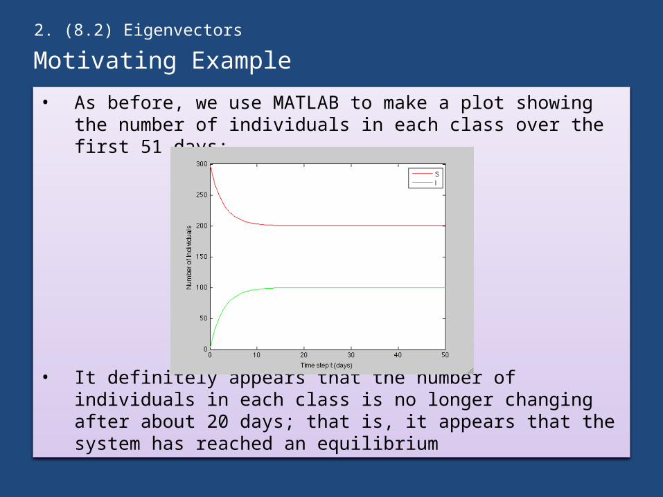
• As before, we use MATLAB to make a plot showing the number of individuals in each class over the first 51 days:

• It definitely appears that the number of individuals in each class is no longer changing after about 20 days; that is, it appears that the system has reached an equilibrium


Motivating Example

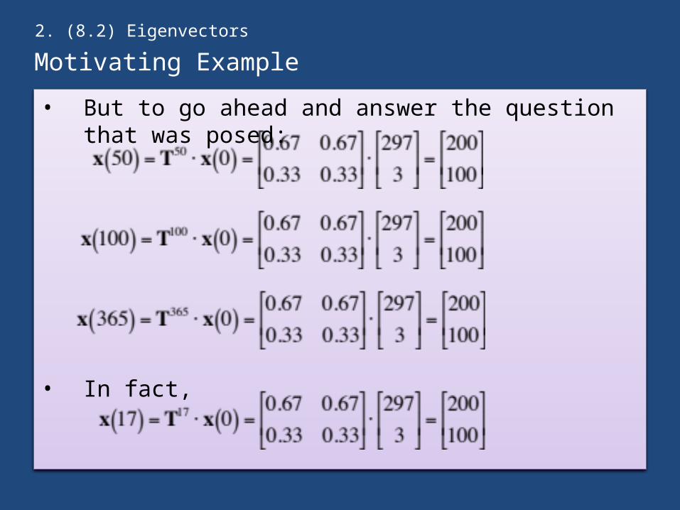
• But to go ahead and answer the question that was posed:

• In fact,


Motivating Example

• So, the vector [200 100]T is an eigenvector for the given transfer matrix.

• While the population structure is at equilibrium, this does not mean that individuals are no longer moving between the susceptible and infected classes

• There is still movement between the classes, however, the movement is such that the number in each class remains constant

• While looking at such a plot is helpful, we need to develop a mathematical method for determining this eigenvector

• Suppose, then, that we don’t know the equilibrium distribution


Motivating Example

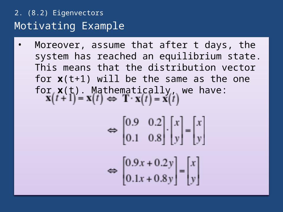
• Moreover, assume that after t days, the system has reached an equilibrium state. This means that the distribution vector for x(t+1) will be the same as the one for x(t). Mathematically, we have:


Motivating Example

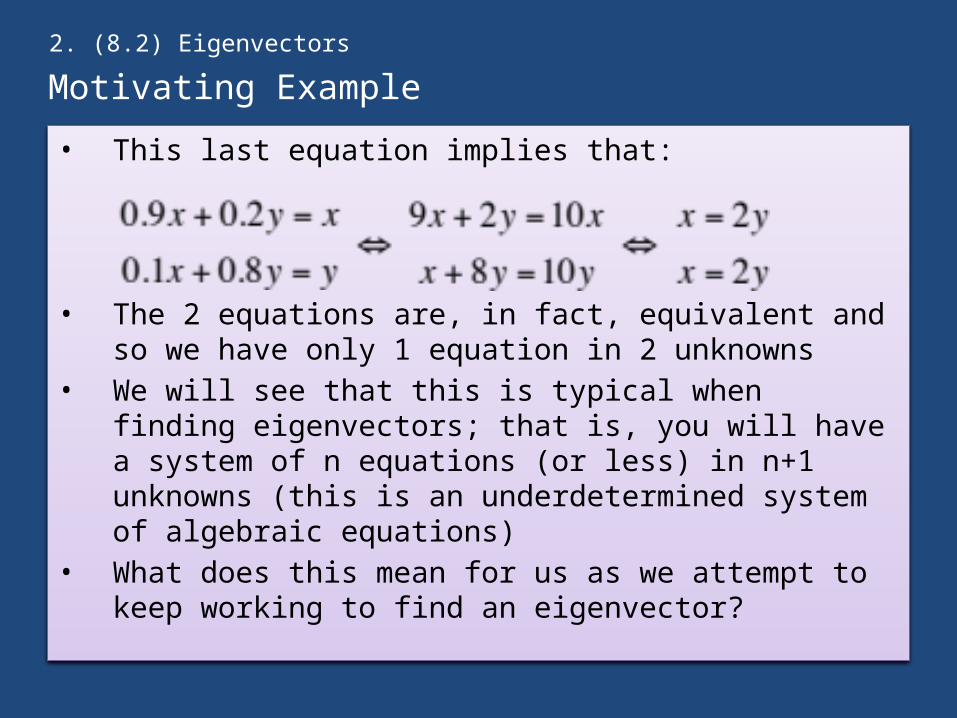
• This last equation implies that:

• The 2 equations are, in fact, equivalent and so we have only 1 equation in 2 unknowns

• We will see that this is typical when finding eigenvectors; that is, you will have a system of n equations (or less) in n+1 unknowns (this is an underdetermined system of algebraic equations)

• What does this mean for us as we attempt to keep working to find an eigenvector?


Motivating Example

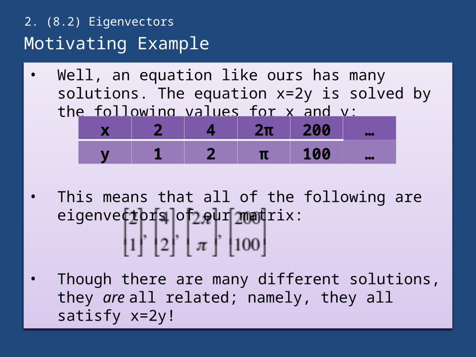
• Well, an equation like ours has many solutions. The equation x=2y is solved by the following values for x and y:

• This means that all of the following are eigenvectors of our matrix:

• Though there are many different solutions, they are all related; namely, they all satisfy x=2y!


x 2 4 2π 200 …y 1 2 π 100 …

Motivating Example

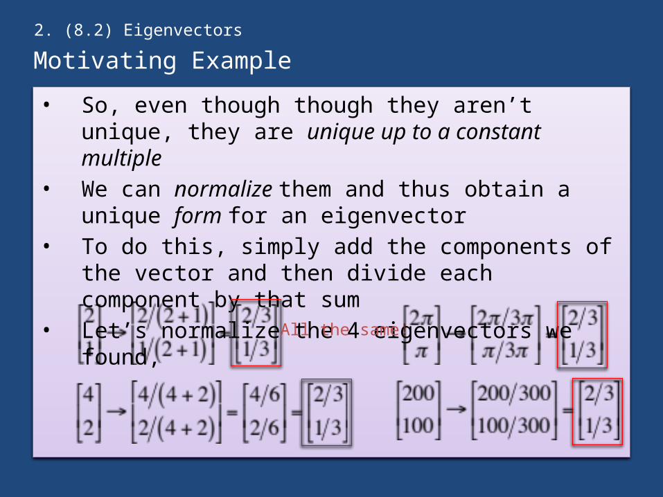
• So, even though though they aren’t unique, they are unique up to a constant multiple

• We can normalize them and thus obtain a unique form for an eigenvector

• To do this, simply add the components of the vector and then divide each component by that sum

• Let’s normalize the 4 eigenvectors we found,


All the same!

Motivating Example

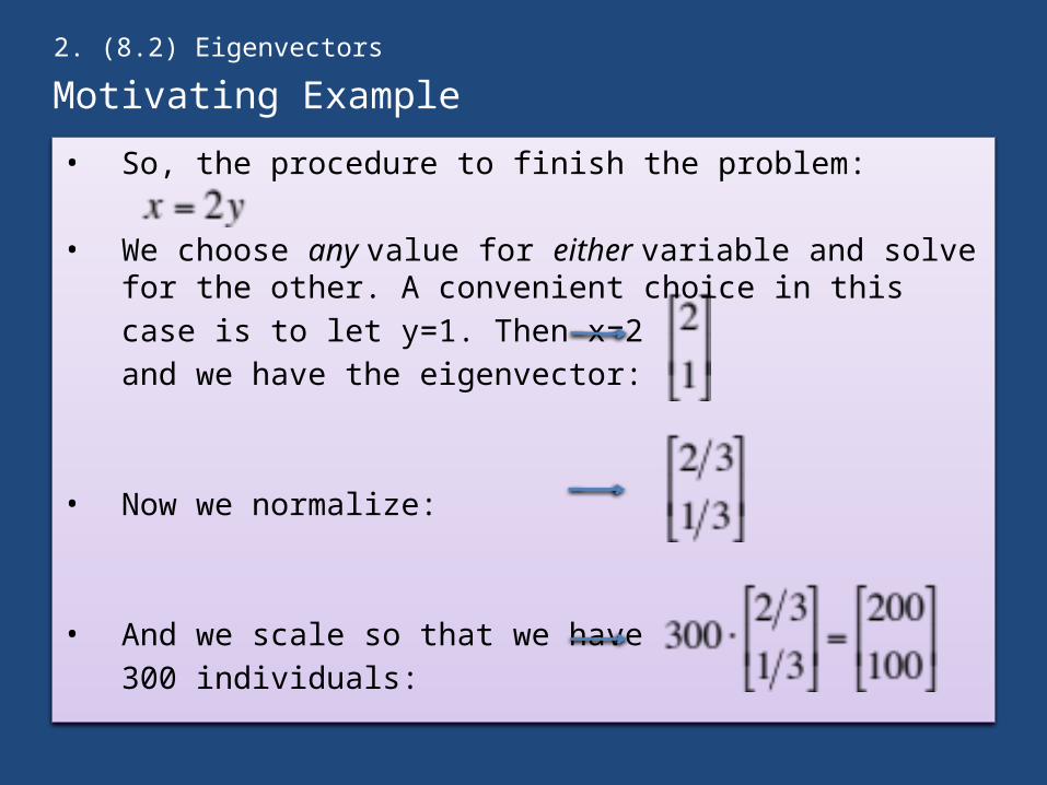
• So, the procedure to finish the problem:

• We choose any value for either variable and solve for the other. A convenient choice in this case is to let y=1. Then x=2and we have the eigenvector:

• Now we normalize:

• And we scale so that we have300 individuals:


Homework Exercise 8.8

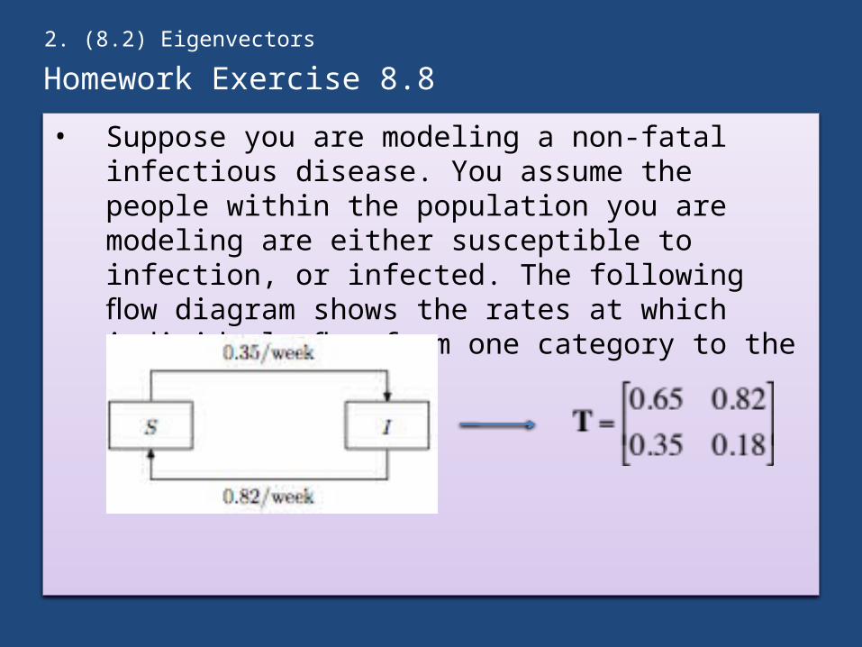
• Suppose you are modeling a non-fatal infectious disease. You assume the people within the population you are modeling are either susceptible to infection, or infected. The following flow diagram shows the rates at which individuals flow from one category to the other:



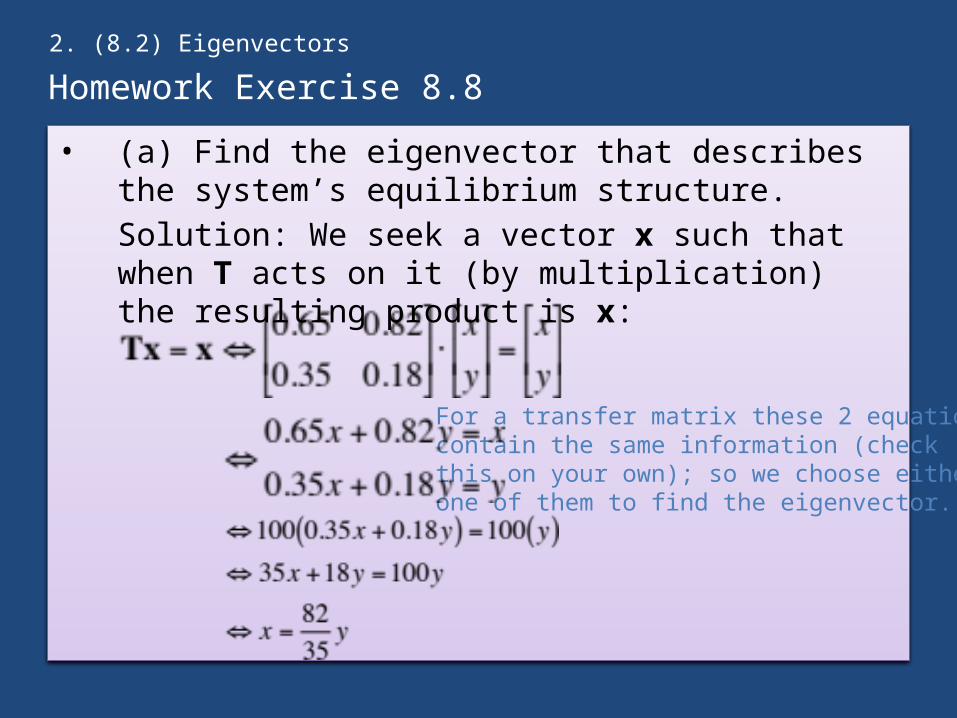
• (a) Find the eigenvector that describes the system’s equilibrium structure.Solution: We seek a vector x such that when T acts on it (by multiplication) the resulting product is x:


For a transfer matrix these 2 equationscontain the same information (checkthis on your own); so we choose eitherone of them to find the eigenvector.


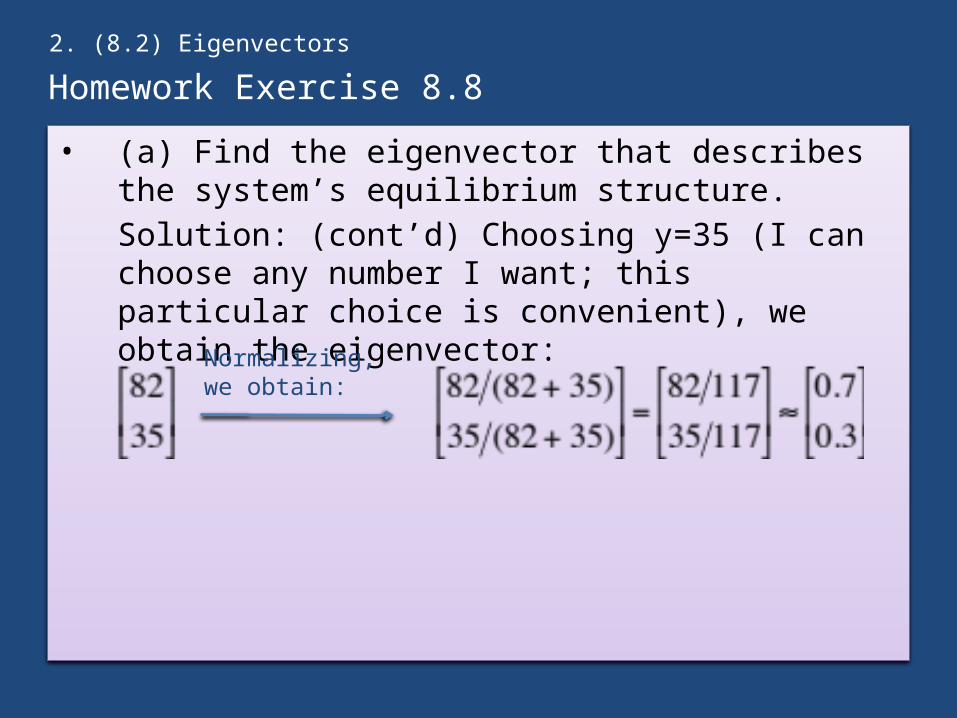
• (a) Find the eigenvector that describes the system’s equilibrium structure.Solution: (cont’d) Choosing y=35 (I can choose any number I want; this particular choice is convenient), we obtain the eigenvector:


Normalizing, we obtain:


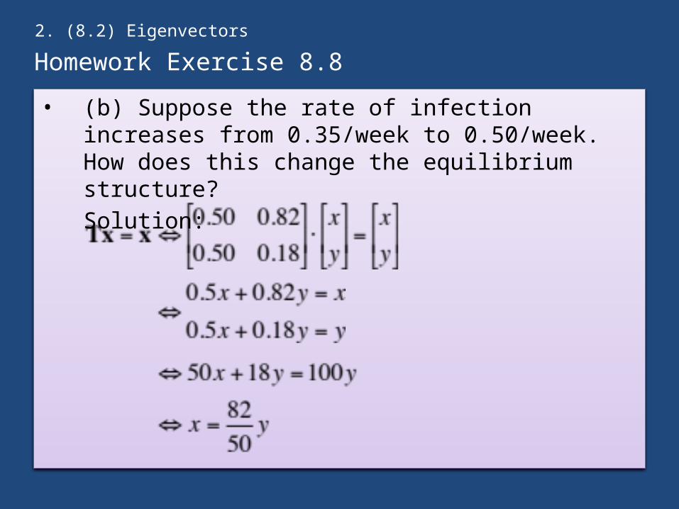
• (b) Suppose the rate of infection increases from 0.35/week to 0.50/week. How does this change the equilibrium structure?Solution:



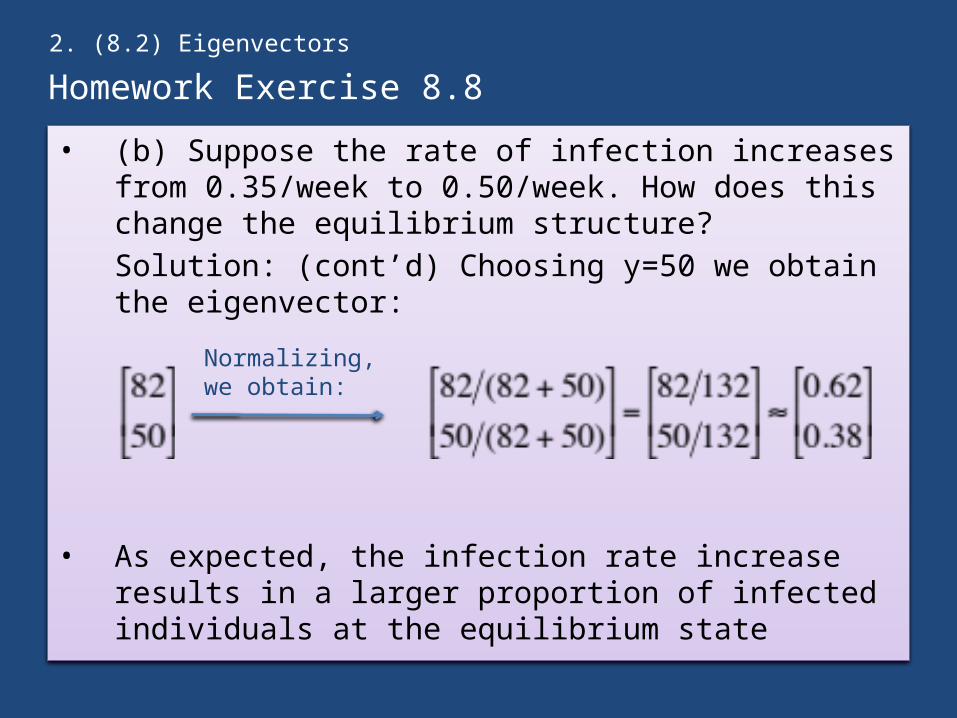
• (b) Suppose the rate of infection increases from 0.35/week to 0.50/week. How does this change the equilibrium structure?Solution: (cont’d) Choosing y=50 we obtain the eigenvector:

• As expected, the infection rate increase results in a larger proportion of infected individuals at the equilibrium state




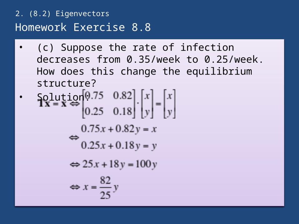
• (c) Suppose the rate of infection decreases from 0.35/week to 0.25/week. How does this change the equilibrium structure?

• Solution:



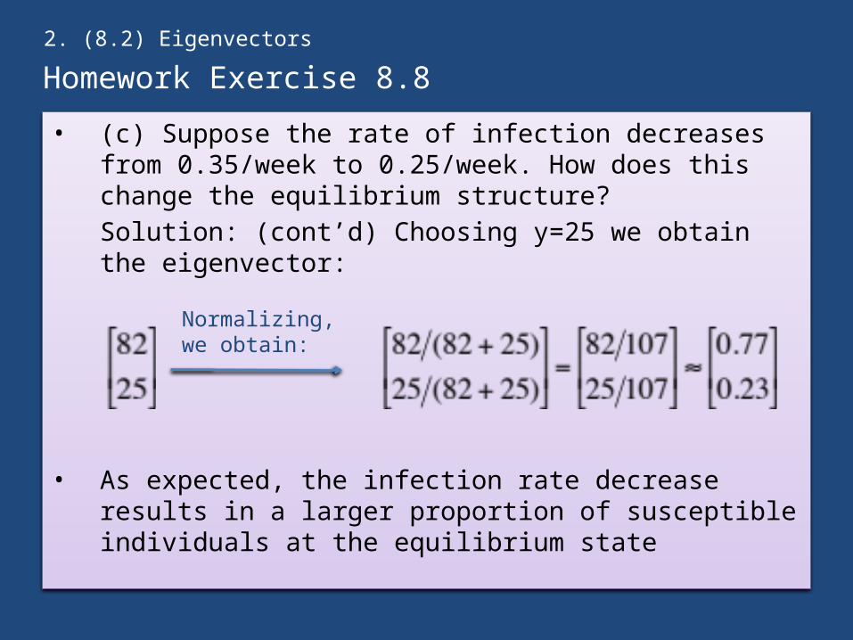
• (c) Suppose the rate of infection decreases from 0.35/week to 0.25/week. How does this change the equilibrium structure?Solution: (cont’d) Choosing y=25 we obtain the eigenvector:

• As expected, the infection rate decrease results in a larger proportion of susceptible individuals at the equilibrium state



Example 7.5

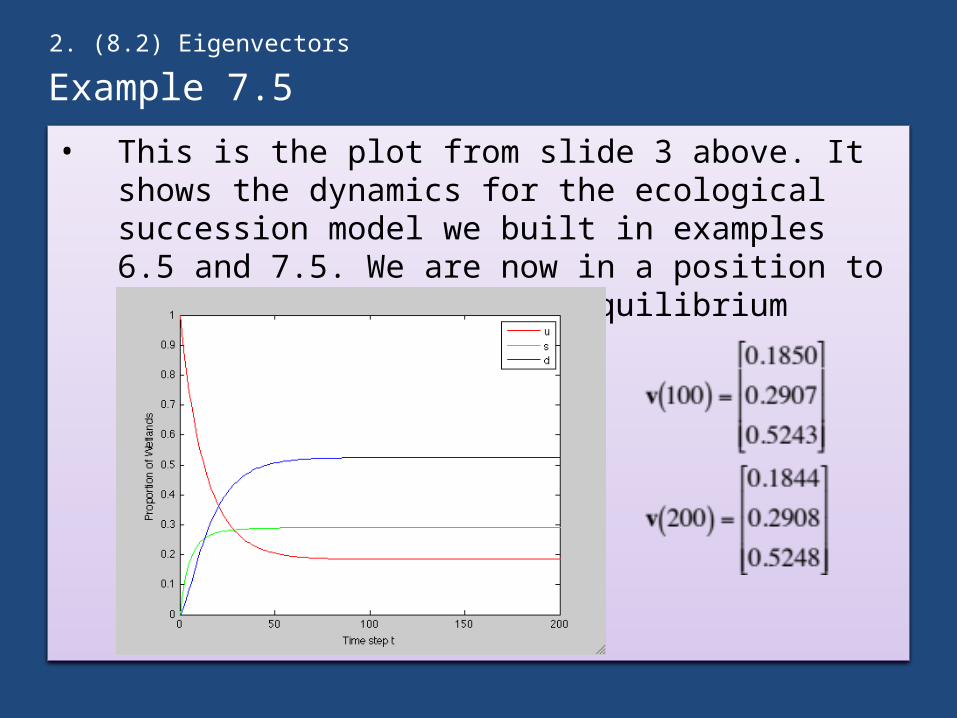
• This is the plot from slide 3 above. It shows the dynamics for the ecological succession model we built in examples 6.5 and 7.5. We are now in a position to determine the long term equilibrium structure mathematically.


Example 7.5


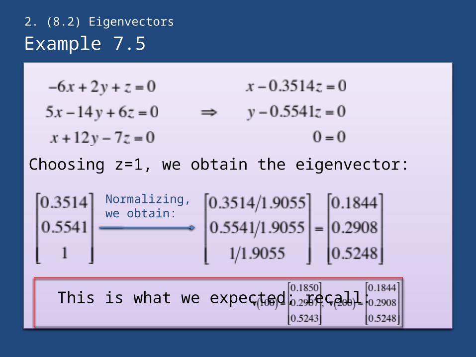
Example 7.5

Choosing z=1, we obtain the eigenvector:

This is what we expected; recall:



What about different initial conditions?

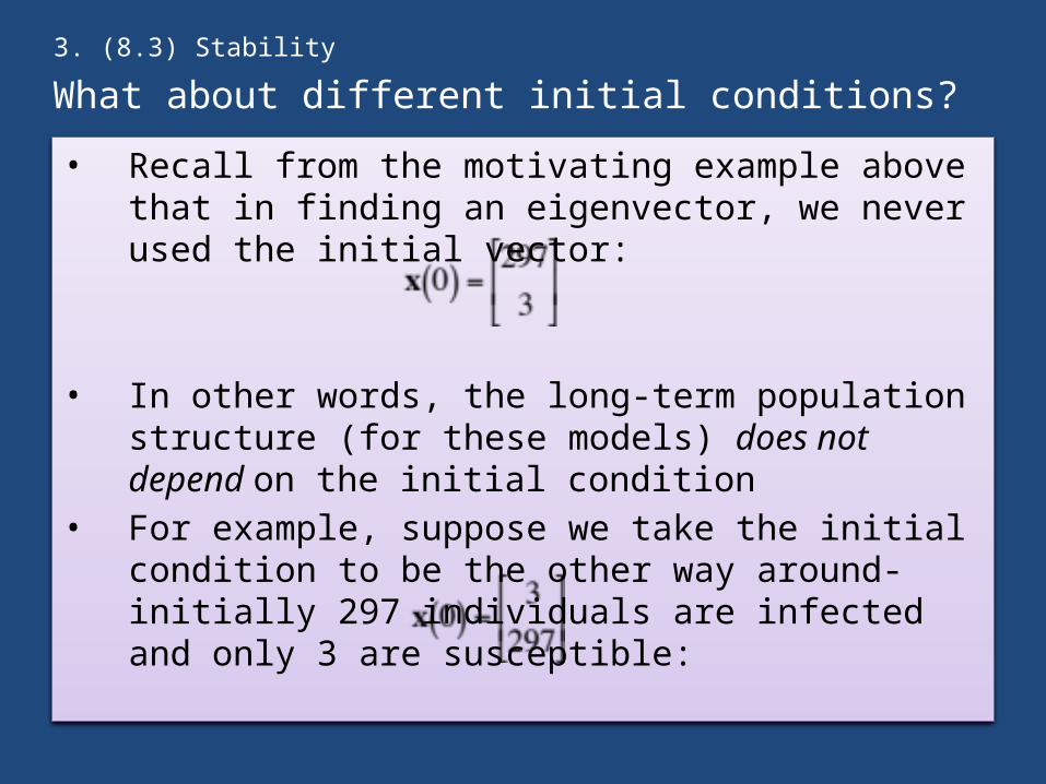
• Recall from the motivating example above that in finding an eigenvector, we never used the initial vector:

• In other words, the long-term population structure (for these models) does not depend on the initial condition

• For example, suppose we take the initial condition to be the other way around- initially 297 individuals are infected and only 3 are susceptible:

3. (8.3) Stability


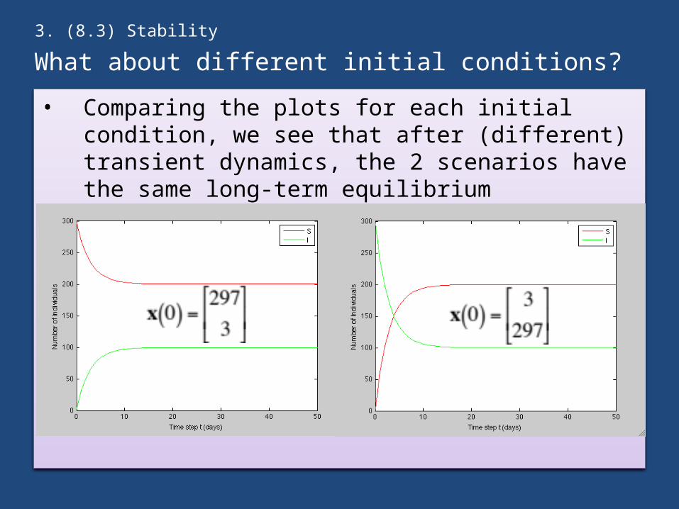
• Comparing the plots for each initial condition, we see that after (different) transient dynamics, the 2 scenarios have the same long-term equilibrium structure:

3. (8.3) Stability


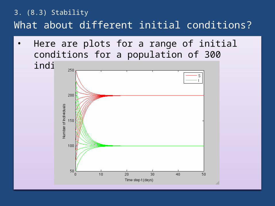
• Here are plots for a range of initial conditions for a population of 300 individuals:

3. (8.3) Stability


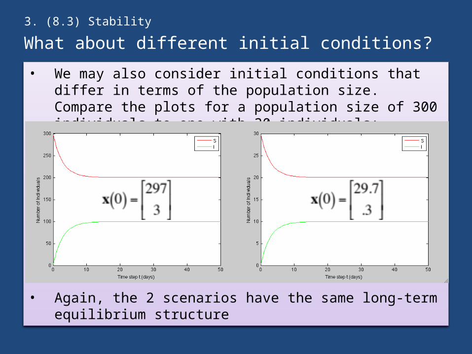
• We may also consider initial conditions that differ in terms of the population size. Compare the plots for a population size of 300 individuals to one with 30 individuals:

• Again, the 2 scenarios have the same long-term equilibrium structure

3. (8.3) Stability

Homework

• Chapter 8: 8.1-8.10

Documents

Chapter 8: Long-Term Dynamics or Equilibrium 1.(8.1) Equilibrium 2.(8.2) Eigenvectors 3.(8.3) Stability 1.(8.1) Equilibrium 2.(8.2) Eigenvectors 3.(8.3)