Chapter 8 Dynamic stability analysis II Longitudinal …...Flight dynamics –II Prof. E.G. Tulapurkara Stability and control Dept. of Aerospace Engg., IIT Madras 1 Chapter 8 Dynamic

Flight dynamics –II Prof. E.G. Tulapurkara

Stability and control

Dept. of Aerospace Engg., IIT Madras 1

Chapter 8

Dynamic stability analysis – II – Longitudinal motion - 2

Lecture 29

Topics

8.5 Iterative solution of characteristic equation

Example 8.2

8.6 Routh’s criteria

8.7 Damping and rate of divergence when root is real

Example 8.3

8.8 Damping, rate of divergence, period of oscillation and number of cycles

for halving or doubling the amplitude when roots constitute a complex

pair

8.9 Modes of longitudinal motion – short period oscillation (SPO) and long

period oscillation (LPO) or phugoid

8.9.1 Phugoid as slow interchange of kinetic energy and potential energy

8.5 Iterative solution of the characteristic equation

The characteristic equation for the stick-fixed longitudinal motion, given

above, is a fourth degree polynomial. It may be noted that the exact solutions for

polynomial equations are available only up to polynomials of degree three.

Hence, in the present case, with fourth degree polynomial, an iterative procedure

is adopted to obtain the solution. Further, the iterative technique, to be used for a

fourth degree polynomial, depends on the relative magnitudes of the coefficients

of the terms in the polynomial. The characteristic equation of the longitudinal

motion generally has the following features.

(a) The coefficient of λ4 is unity.

(b) The coefficients of λ3 and λ2 are much larger than the coefficient of the λ and

the constant term (see values of B, C, D and E in Eq.8.18).

Reference1.5 Appendix 4, gives the following iterative procedure for solving

polynomial like in Eq.(8.18).




Let, 4 3 2f(λ) = λ + Bλ + Cλ + Dλ + E (8.19)

Now, f(λ) can be expressed as a product of two quadratics i.e.:

2 2f(λ) = (λ + bλ + c) (λ + λ + δ) (8.20)

Expanding R.H.S. of Eq.(8.20) and comparing coefficients of terms in Eqs.

(8.19) and (8.20) gives the following equations.

b + = B

c + b + δ = C

bδ + c = D

cδ = E

(8.21)

Since, the coefficients D and E are generally much smaller than ‘B’ and ‘C’ , the

quantities and δ in Eq.(8.21) are much smaller than ‘b’ and ‘c’ . Hence, the first

approximations of b,c,δ and , denoted by b1, c2, 1δ and 1 are written as :

1

1

1

1 2 2

b B

c C

E Eδ =

c C

cD - bE CD - BE=

c C

(8.22)

Hence, 2 2

2

CD - BE Ef(λ) (λ + Bλ + C) (λ + λ + ) 0

C C (8.23)

The roots of the two quadratics in Eq.(8.23) are obtained.

For the second approximation, b2, c2 , 2δ , and 2 are expressed as:

2 1

2 1 1 1

2 22 2

2

2

2

b B -

c C - b - δ

c D - b E

c

Eδ =

c

(8.24)

The roots of the quadratics obtained using b2 , c2, 2 and δ2 are also worked

out.The procedure is continued till the roots obtained in the two consecutive

approximations do not change significantly in their values.




Example 8.2

An application of the iterative procedure for the characteristic equation for

the case considered in example 8.1 is described below.

From Eq.(8.18): A = 1, B = 5.05, C = 13.15, D = 0.6735 and E = 0.593.

From the set of equations in Eq.(8.22) the first approximation is :

b1 = 5.05, c1 = 13.15, δ1 = (0.593/13.15) = 0.0451, and

γ1 = (13.15 x 0.6735 - 5.05x0.593) / 13.152 = 0.0339

Thus, f(λ) ≈ (λ2+5.05λ+13.15) (λ2 + 0.0339λ + 0.0451)

The roots of the two quadratics are:

λ1,2 = -2.525 ± i 2.602, λ3,4 = -0.01695 ± i 0.2117

From the set of equations in Eq.(8.24) the second approximation is:

b2 = B - γ1 = 5.05 – 0.0339 = 5.0161.

Similarly, c2=12.934, γ2 = 0.0343 and δ2 = 0.0458.

The roots of the quadratic obtained using b2, c2, γ2 and δ2 are:

λ1,2 = -2.508 ± i 2.578 , λ3,4 = -0.01715 ± i 0.213

Carrying out the iteration once more, the roots after the third approximation are:

λ1,2 = -2.508 ± i 2.577,

λ3,4 = -0.01715 ± i 0.2135.

The values of the roots do not seem to change significantly from the second to

the third iteration and the iterative procedure can be stopped.

Remarks:

i) In section 8.10 the equations of motion are expressed in state space

variable form and then the roots of the characteristics equation are

obtained by using commercially available computational packages like

Matlab.

ii) It is observed that the four roots of the characteristic equation for the

given flight condition, consist of two pairs of complex roots. The real parts

of both the roots are negative and hence the airplane has dynamic

stability for the given flight conditions and configuration. A discussion on

the modes of longitudinal motion is given in section 8.9.




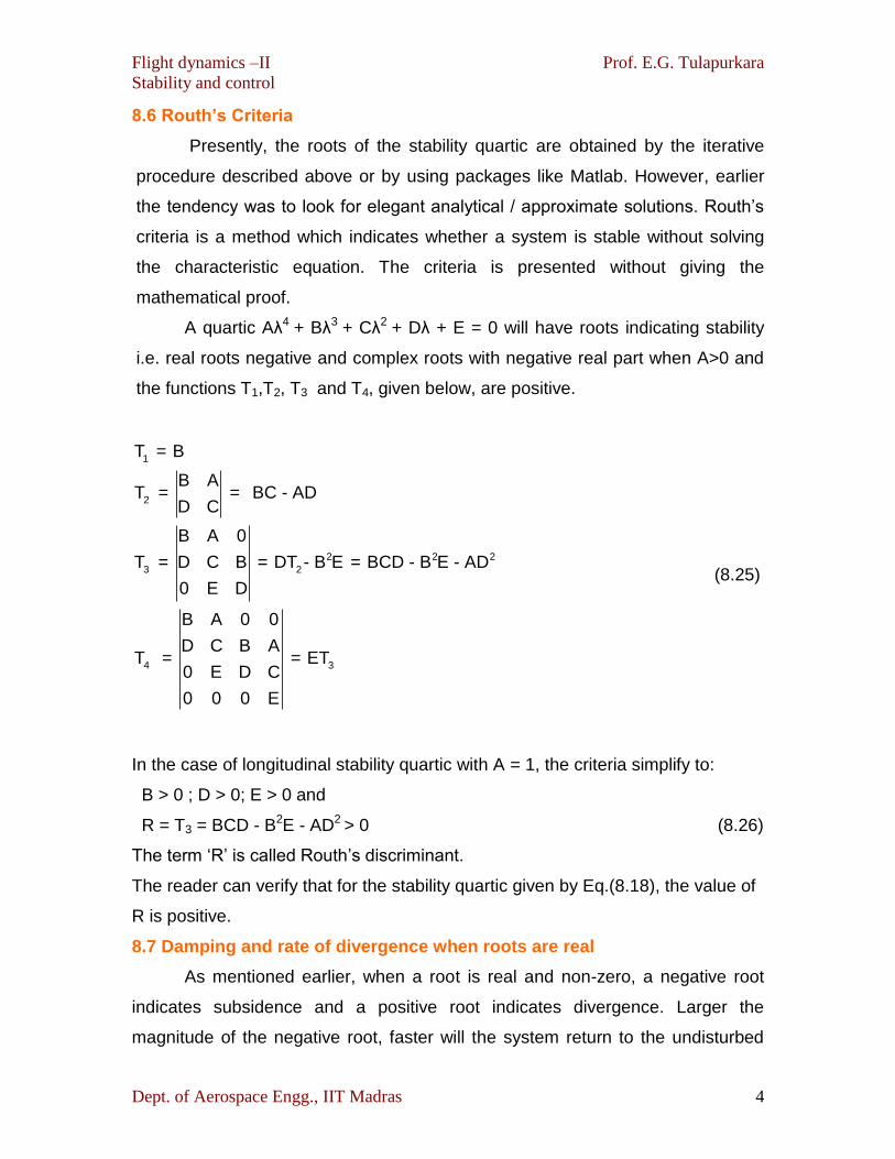
8.6 Routh’s Criteria

Presently, the roots of the stability quartic are obtained by the iterative

procedure described above or by using packages like Matlab. However, earlier

the tendency was to look for elegant analytical / approximate solutions. Routh’s

criteria is a method which indicates whether a system is stable without solving

the characteristic equation. The criteria is presented without giving the

mathematical proof.

A quartic Aλ4 + Bλ3 + Cλ2 + Dλ + E = 0 will have roots indicating stability

i.e. real roots negative and complex roots with negative real part when A>0 and

the functions T1,T2, T3 and T4, given below, are positive.

1

2

2 2 2

3 2

4 3

T = B

B AT = = BC - AD

D C

B A 0

T = D C B = DT - B E = BCD - B E - AD

0 E D

B A 0 0

D C B AT = = ET

0 E D C

0 0 0 E

(8.25)

In the case of longitudinal stability quartic with A = 1, the criteria simplify to:

B > 0 ; D > 0; E > 0 and

R = T3 = BCD - B2E - AD2 > 0 (8.26)

The term ‘R’ is called Routh’s discriminant.

The reader can verify that for the stability quartic given by Eq.(8.18), the value of

R is positive.

8.7 Damping and rate of divergence when roots are real

As mentioned earlier, when a root is real and non-zero, a negative root

indicates subsidence and a positive root indicates divergence. Larger the

magnitude of the negative root, faster will the system return to the undisturbed




position. This is clear from Eq.(8.15), which shows that the response of the

system corresponding to the root λ1 is 11 1λ te . At t = 0, the amplitude of the

response is 11 . Further, when 1λ is negative, the term 1λ te indicates that the

amplitude would decrease exponentially with time (Fig 8.1b). The time when the

amplitude decreases to half of its value at t = 0, is a measure of the damping.

This time is denoted by t1/2. This quantity (t1/2) is obtained from the following

equation.

For the sake of generality the root is denoted by λ instead of 1λ .

1/2t λ 1e =

2

Or 1/2t = (ln2) / λ = 0.693 / λ (8.27)

When the root is positive, the amplitude increases exponentially with time

(Fig 8.1a). The time when the amplitude is twice the value at t = 0, is a measure

of divergence. This time is denoted by t2. This quantity (t2) is obtained from the

following equation.

2t λe = 2; ; Note λ is positive

Or t2 = (ln 2) / λ = 0.693 / λ (8.28)

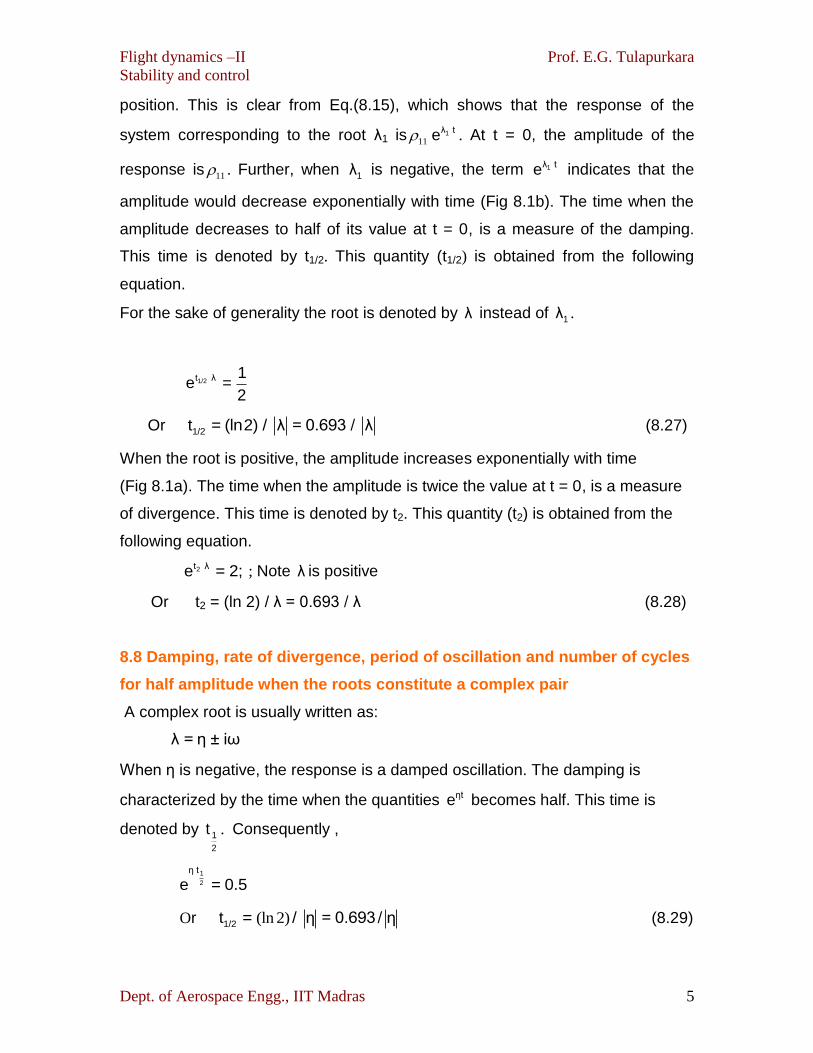
8.8 Damping, rate of divergence, period of oscillation and number of cycles

for half amplitude when the roots constitute a complex pair

A complex root is usually written as:

λ = η ± iω

When η is negative, the response is a damped oscillation. The damping is

characterized by the time when the quantities ηte becomes half. This time is

denoted by 1

2

t . Consequently ,

1

2

η t

e = 0.5

Or (ln 2)1/2t = / η = 0.693/ η (8.29)




When η is positive, the response is a divergent oscillation. The time when the

term ηte equals two is a measure of the rate of divergence. This time is denoted

by t2. It is easy to show that :

2t = ln 2 /η = 0.693/η (8.30)

The time period of the oscillation (P) is given by

P = 2π / ω (8.31)

When η is negative, the number of cycles from t = 0 to t1/2 is denoted by N1/2

and equals:

1/2 1/2N = t / P (8.32)

Similarly, when η is positive, the number of cycles from t = 0 to t2 is denoted by

N2 and equals:

2 2N = t / P (8.33)

Example 8.3

Applying the above formulae, the quantities t1/2 , P, N1/2 corresponding to the

two roots obtained in example 8.2 are:

a) λ1,2 = -2.508 ± i 2.578:

t1/2 = 0.693/2.508 = 0.276 s,

P = 2π /2.578 = 2.436 s, N1/2 = 0.276 / 2.436 = 0.113 cycles

b) λ3,4 = - 0.01715 ± i 0.2135:

t1/2 = 0.693 / 0.01715 = 40.4s

P = 2π / 0.2135 = 29.4 s, N1/2 = 40.4 / 29.4 = 1.37 cycles

8.9 Modes of longitudinal motion – short period oscillation (SPO) and long

period oscillation (LPO) / phugoid

The motions represented by the different roots of the characteristic

equation are called the corresponding modes. For the longitudinal motion the

characteristic equation generally has two complex roots. One of them has a short

time period and is heavily damped (refer to examples 8.2 and 8.3). This mode is

called short period oscillation (SPO). The other mode has a long time period and

low damping (refer to examples 8.2 and 8.3).This mode is called long period




oscillation(LPO). Because of low damping it takes a long time to subside or die

down. However, when the period is long, the pilot has enough time to take

corrective action to restore equilibrium. This mode is also called phugoid. To

appreciate the features of these two modes, the response of Navion to a

disturbance, as given in Reference 1.12, chapter 6 is presented in Figs.8.3a & b

and 8.4 a & b.The disturbance consists of Δα = 50 and 0Δu = 0.1u = 17.6 ft s -1 or

5.364 ms-1.

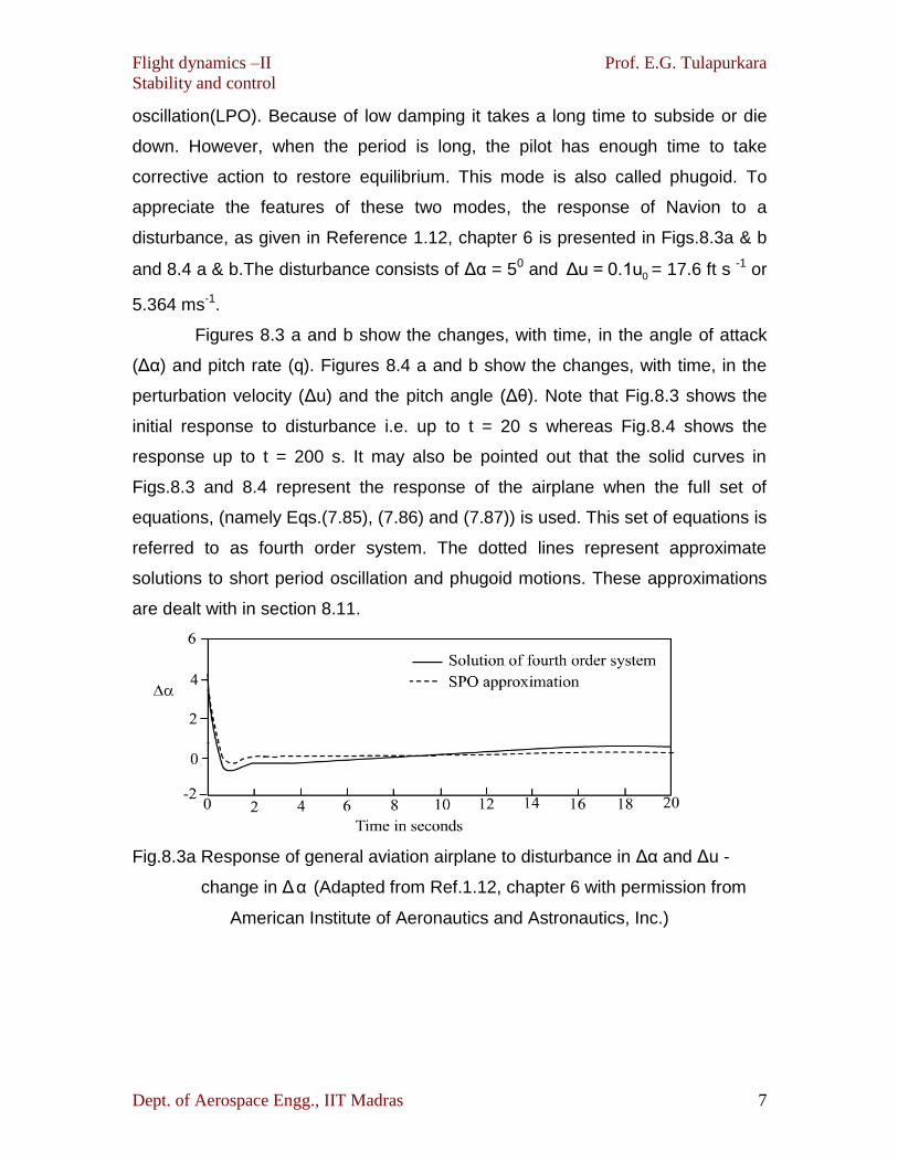
Figures 8.3 a and b show the changes, with time, in the angle of attack

(Δα) and pitch rate (q). Figures 8.4 a and b show the changes, with time, in the

perturbation velocity (Δu) and the pitch angle (Δθ). Note that Fig.8.3 shows the

initial response to disturbance i.e. up to t = 20 s whereas Fig.8.4 shows the

response up to t = 200 s. It may also be pointed out that the solid curves in

Figs.8.3 and 8.4 represent the response of the airplane when the full set of

equations, (namely Eqs.(7.85), (7.86) and (7.87)) is used. This set of equations is

referred to as fourth order system. The dotted lines represent approximate

solutions to short period oscillation and phugoid motions. These approximations

are dealt with in section 8.11.

Fig.8.3a Response of general aviation airplane to disturbance in Δα and Δu -

change in Δα (Adapted from Ref.1.12, chapter 6 with permission from

American Institute of Aeronautics and Astronautics, Inc.)




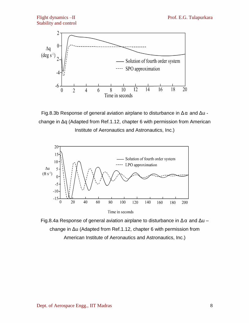
Fig.8.3b Response of general aviation airplane to disturbance in Δα and Δu -

change in Δq (Adapted from Ref.1.12, chapter 6 with permission from American

Institute of Aeronautics and Astronautics, Inc.)

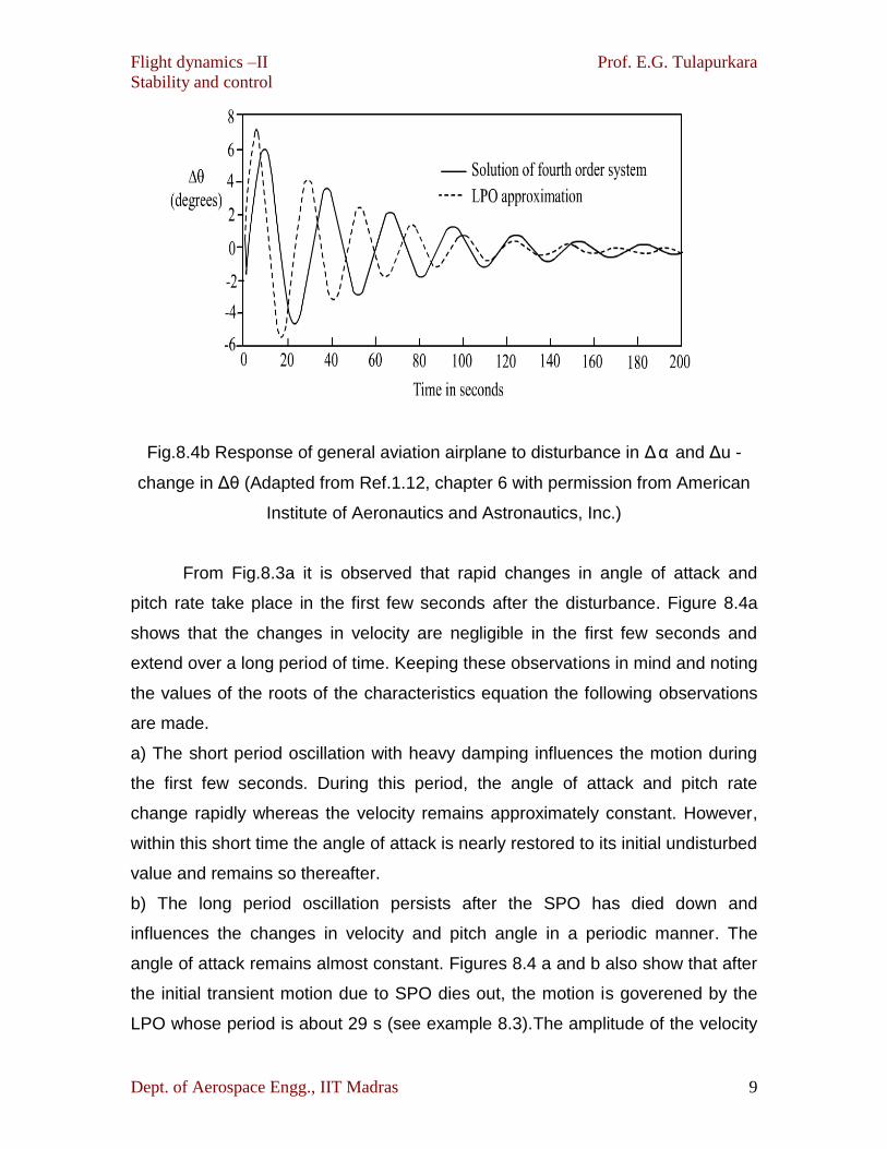
Fig.8.4a Response of general aviation airplane to disturbance in Δα and Δu –

change in Δu (Adapted from Ref.1.12, chapter 6 with permission from

American Institute of Aeronautics and Astronautics, Inc.)




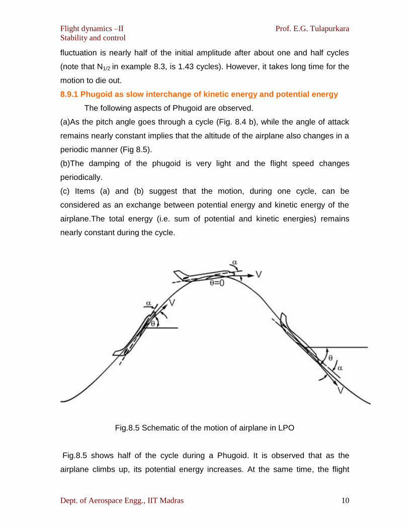
Fig.8.4b Response of general aviation airplane to disturbance in Δα and Δu -

change in Δθ (Adapted from Ref.1.12, chapter 6 with permission from American

Institute of Aeronautics and Astronautics, Inc.)

From Fig.8.3a it is observed that rapid changes in angle of attack and

pitch rate take place in the first few seconds after the disturbance. Figure 8.4a

shows that the changes in velocity are negligible in the first few seconds and

extend over a long period of time. Keeping these observations in mind and noting

the values of the roots of the characteristics equation the following observations

are made.

a) The short period oscillation with heavy damping influences the motion during

the first few seconds. During this period, the angle of attack and pitch rate

change rapidly whereas the velocity remains approximately constant. However,

within this short time the angle of attack is nearly restored to its initial undisturbed

value and remains so thereafter.

b) The long period oscillation persists after the SPO has died down and

influences the changes in velocity and pitch angle in a periodic manner. The

angle of attack remains almost constant. Figures 8.4 a and b also show that after

the initial transient motion due to SPO dies out, the motion is goverened by the

LPO whose period is about 29 s (see example 8.3).The amplitude of the velocity




fluctuation is nearly half of the initial amplitude after about one and half cycles

(note that N1/2 in example 8.3, is 1.43 cycles). However, it takes long time for the

motion to die out.

8.9.1 Phugoid as slow interchange of kinetic energy and potential energy

The following aspects of Phugoid are observed.

(a)As the pitch angle goes through a cycle (Fig. 8.4 b), while the angle of attack

remains nearly constant implies that the altitude of the airplane also changes in a

periodic manner (Fig 8.5).

(b)The damping of the phugoid is very light and the flight speed changes

periodically.

(c) Items (a) and (b) suggest that the motion, during one cycle, can be

considered as an exchange between potential energy and kinetic energy of the

airplane.The total energy (i.e. sum of potential and kinetic energies) remains

nearly constant during the cycle.

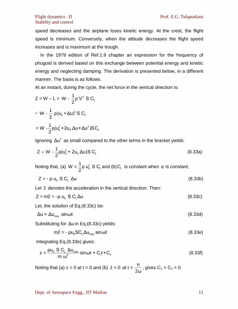
Fig.8.5 Schematic of the motion of airplane in LPO

Fig.8.5 shows half of the cycle during a Phugoid. It is observed that as the

airplane climbs up, its potential energy increases. At the same time, the flight




speed decreases and the airplane loses kinetic energy. At the crest, the flight

speed is minimum. Conversely, when the altitude decreases the flight speed

increases and is maximum at the trough.

In the 1979 edition of Ref.1.9 chapter an expression for the frequency of

phugoid is derived based on this exchange between potential energy and kinetic

energy and neglecting damping. The derivation is presented below, in a different

manner. The basis is as follows.

At an instant, during the cycle, the net force in the vertical direction is:

Z = W – L = 2

L

1W - ρ V S C

2

= 2

0 L

1W - ρ(u +Δu) S C

2

2 2

0 0 L

1= W - ρ(u +2u Δu+Δu )SC

2

Ignoring 2Δu as small compared to the other terms in the bracket yields:

2

0 0 L

1Z W - ρ(u + 2u Δu)S C

2 (8.33a)

Noting that, (a) 2

0 L

1W = ρ u S C

2and (b) LC is constant when α is constant,

0 LZ = - ρ u S C Δu (8.33b)

Let z denotes the acceleration in the vertical direction. Then:

0 LZ = mz = -ρ u S C Δu (8.33c)

Let, the solution of Eq.(8.33c) be:

maxΔu = Δu sinωt (8.33d)

Substituting for Δu in Eq.(8.33c) yields:

0 L maxmz = - ρu SC Δu sinωt (8.33e)

Integrating Eq.(8.33e) gives:

0 L max1 22

ρu S C Δuz = sinωt + C t+C

m ω (8.33f)

Noting that (a) z = 0 at t = 0 and (b) z = 0 at t = π

2ω, gives C1 = C2 = 0




Or 0 L max

2

ρ u S C Δuz =

m ω (8.33g)

Now, the altitude changes as z changes and the potential energy changes with it.

The maximum change in potential energy max

ΔPE is mg (zmax – zmin). From

Eq.(8.33g)

0 L max

2max

2 g ρ u S C ΔuΔPE =

ω (8.33h)

The maximum change in the kinetic energy max

ΔKE is:

22

0 max 0 maxmax

1 1ΔKE = m (u +Δu ) - m u -Δu

2 2 0 max= 2mu Δu (8.33i)

Since, the phugoid is approximated as an exchange between PE and KE,

max max

ΔPE = ΔKE

Or 0 L max

2

2gρu SC Δu

ω = 0 max2mu Δu (8.33j)

Substituting L 2

0

2mgC =

ρu S in Eq.(8.33j) yields:

0

gω = 2 rad/s

u (8.33 k)

This interesting result shows that the frequency of phugoid is inversely

proportional to u0 or the time period of the oscillation is proportional to u0. The

result is independent of the airplane characteristics because the damping (which

depends on CD) has been ignored in the analysis.

In subsection 8.11.2 the same expression for ω is obtained by simplifying

the equations of motion.

Remark: The website: www.youtube.com has many videos on Phugoid. One of

them ( PH-Lab (3/7)) indicates phugoid motion as the movement of horizon when

photographed from inside the airplane. See also videos on short period

oscillation.

http://www.youtube.com/

Documents

Chapter 8 Dynamic stability analysis II Longitudinal …...Flight dynamics –II Prof. E.G. Tulapurkara Stability and control Dept. of Aerospace Engg., IIT Madras 1 Chapter 8 Dynamic