Embed Size (px)
Citation preview
Chapter 8
Discrete probability and the laws ofchance
8.1 Introduction
In this chapter we lay the groundwork for calculations and rules governing simple discrete probabil-ities. These steps will be essential to developing the skills to analyzing and understanding problemsof genetic diseases, genetic codes, and a vast array of other phenomena where the laws of chanceintersect the the processes of biological systems. To gain experience with probability, it is importantto see simple examples. We start this introduction with experiments that can be easily reproducedand tested by the reader.
8.2 Simple experiments
Consider the following experiment: We flip a coin and observe any one of two possible results:“heads” (H) or “tails” (T). A fair coin is one for which these results are equally likely. Similarly,consider the experiment of rolling a dice: A six-sided dice can land on any of its six faces, sothat a “single experiment” has six possible outcomes. We anticipate getting each of the resultswith an equal probability, i.e. if we were to repeat the same experiment many many times, wewould expect that, on average, the six possible events would occur with similar frequencies. Wesay that the events are random and unbiased for “fair” dice. How likely are we to roll a 5 anda 6 in successive experiments? A five or a six? If we toss a coin ten times, how probable is itthat we get 8 out of ten heads? For a given experiment such as the one described here, we areinterested in quantifying how likely it is that a certain event is obtained. Our goal in this chapter isto make more precise our notion of probability, and to examine ways of quantifying and computingprobabilities for experiments such as these. To motivate this investigation, we first look at resultsof a real experiment performed in class by students.
v.2005.1 - January 5, 2009 1
Math 103 Notes Chapter 8
8.3 Empirical probability
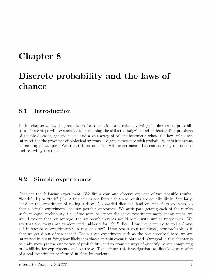
Each student in a class of N = 121 individuals was asked to toss a penny 10 times. The studentswere then asked to record their results and to indicate how many heads they had obtained in thissequence of tosses. (Note that the order of the heads was not taken into account, only how manywere obtained out of the 10 tosses.) The table shown below specifies the number, k, of heads(column 1), the number, xk, of students who responded that they had obtained that many heads(column 2). In column (4) we compute the fraction of the class p(xk) = xk/N who got exactly kheads. In column (3) we display a cumulative number of students who got any number up to andincluding k heads, and then in column (5) we compute the cumulative fraction of the class whogot any number up to and including k heads. We will henceforth associate the fraction with theempirical probability of k heads. In the last column we include the cumulative probability, i.e. thesum of the probabilities of getting any number up to k heads.
Number of heads frequency Cumulative probability cumulative probability
k xk
k∑
i
xi p(xk) = xk/N
k∑
i
p(xi)
0 0 0 0.00 0.001 1 1 0.0083 0.00832 2 3 0.0165 0.02483 10 13 0.0826 0.10744 27 40 0.2231 0.33065 26 66 0.2149 0.54556 34 100 0.2810 0.82647 14 114 0.1157 0.94218 7 121 0.0579 1.009 0 121 0.00 1.0010 0 121 0.00 1.00
Table 8.1: Results of a real experiment carried out by 121 students in this mathematics course.Each student tossed a coin 10 times. We recorded the number of students who got 0, 1, 2, etcheads. The fraction of the class that got each outcome is identified with the (empirical) probabilityof that outcome. See Figure 8.1 for the same data presented graphically.
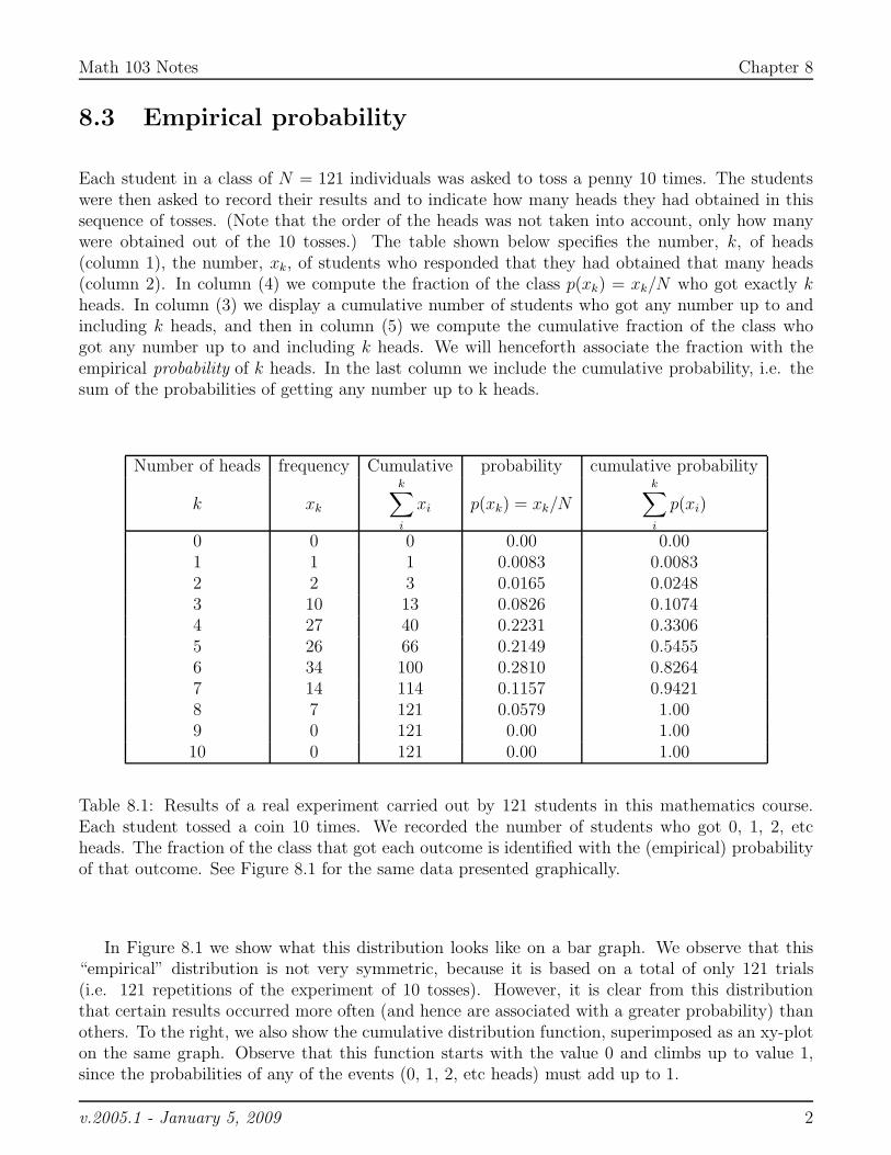
In Figure 8.1 we show what this distribution looks like on a bar graph. We observe that this“empirical” distribution is not very symmetric, because it is based on a total of only 121 trials(i.e. 121 repetitions of the experiment of 10 tosses). However, it is clear from this distributionthat certain results occurred more often (and hence are associated with a greater probability) thanothers. To the right, we also show the cumulative distribution function, superimposed as an xy-ploton the same graph. Observe that this function starts with the value 0 and climbs up to value 1,since the probabilities of any of the events (0, 1, 2, etc heads) must add up to 1.
v.2005.1 - January 5, 2009 2
Math 103 Notes Chapter 8
number of heads (k)
empirical probability of k heads in 10 tosses
0.0 10.0
0.0
0.4
number of heads (k)
Cumulative distribution
0.0 10.0
0.0
1.0
Figure 8.1: The data from Table 8.1 is shown plotted on this graph. A total of N = 121 people wereasked to toss a coin n = 10 times. In the bar graph (left), the horizontal axis reflects k, the number,of heads (H) that came up during those 10 coin tosses. The vertical axis reflects the fraction p(xk)of the class that achieved that particular number of heads. The same bar graph is shown on theright, together with the cumulative function that sums up the values from left to right.
v.2005.1 - January 5, 2009 3
Math 103 Notes Chapter 8
8.4 Mean and variance of a probability distribution
In a previous chapter, we considered distributions of grades and computed a mean (also calledaverage) of that distribution. The identical concept applies in the distributions discussed in thecontext of probability, but here we interchangeably use the terminology mean or average valueor expected value.
Suppose we toss a coin n times and let xi stand for the number of heads that are obtained inthose n tosses. Then xi can take on the values xi = 0, 1, 2, 3, . . . n. Let p(xi) be the probability ofobtaining exactly xi heads. By analogy to ideas in a previous chapter, we would define the mean(or average or expected value), x̄ of the probability distribution by the ratio
x̄ =
∑ni=0
xip(xi)∑n
i=0p(xi)
.
However, this expression can be simplified by observing that, according to property (2) of discreteprobability, the denominator is just
n∑
i=0
p(xi) = 1
This explains the following definition of the expected value.
Definition
The expected value x̄ of a probability distribution (also called the mean or average value) is
x̄ =
n∑
i=0
xip(xi) .
It is important to keep in mind that the expected value or mean is a kind of “average x co-ordinate”, where values of x are weighted by their frequency of occurrence. This is similar to theidea of a center of mass (x positions weighted by masses associated with those positions). Themean is a point on the x axis, representing the “average” outcome of an experiment. (Recall thatin the distributions we are describing, the possible outcomes of some observation or measurementprocess are depicted on the x axis of the graph.) The mean is not the same as the average value ofa function, discussed in an earlier chapter. (In that case, the average is an average y coordinate.)
We also define a numerical quantity that represents the width of the distribution. We define thevariance, V and standard deviation, σ as follows:
v.2005.1 - January 5, 2009 4
Math 103 Notes Chapter 8
The variance, V , of a distribution is
V =n
∑
i=0
(xi − x̄)2p(xi).
where x̄ is the mean. The standard deviation, σ is
σ =√
V .
In the problem sets, we show that the variance can also be expressed in the form
V = M2 − x̄2
where M2 is the second moment of the distribution. Moments of a distribution are defined as thenumbers obtained by summing up products of the probability weighted by powers of x. The j’thmoment, Mj of a distribution is
Mj =n
∑
i=0
(xi)jp(xi).
8.4.1 Example
For the empirical probability distribution shown in Figure 8.1, the mean (expected value) is calcu-lated by performing the following sum, based on the table of events shown above:
x̄ =
10∑
k=0
xkp(xk) = 0(0) + 1(0.0083) + 2(0.0165) + · · · + 8(0.0579) + 9(0) + 10(0) = 5.2149
The mean number of heads in this set of experiments is about 5.2. Intuitively, we would expectthat in a fair coin, half the tosses should produce heads, i.e. on average 5 heads would be obtainedout of 10 tosses. We see from the fact that the empirical distribution is slightly biased, that themean is close to, but not equal to this intuitive theoretical result.
To compute the variance we form the sum
V =10
∑
k=0
(xk − x̄)2p(xk) =10
∑
k=0
(k − 5.2149)2p(k).
Here we have used the mean calculated above and the fact that xk = k. We obtain
V = (0 − 5.2149)2(0) + (1 − 5.2149)2(0.0083) + · · ·+ (9 − 5.2149)2(0) + (10 − 5.2149)2(0) = 2.0530
The standard deviation is then σ =√
V = 1.4328.
v.2005.1 - January 5, 2009 5
Math 103 Notes Chapter 8
8.5 Theoretical probability
Our motivation in what follows it to put results of an experiment into some rational context. Wewould like to be able to predict the distribution of outcomes based on underlying “laws of chance”.Here we will formalize the basic rules of probability, and learn how to assign probabilities to eventsthat consist of repetitions of some basic, simple experiment like the coin toss. Intuitively, we expectthat in tossing a fair coin, half the time we should get H and half the time T. But as seen in ourexperimental results, there can be long repetitions that result in very few H or very many H, farfrom the mean or expected value. How do we assign a theoretical probability to the event that only1 head is obtained in 10 tosses of a coin? This motivates our more detailed study of the laws ofchance and theoretical probability.
As we have seen in our previous example, the probability p assigns a number to the likelihoodof an outcome of an experiment. In the experiment discussed above, that number was the fractionof the students who got a certain number of heads in a coin toss repetition.
8.5.1 Basic definitions of probability
Suppose we label the possible results of the experiment by symbols e1, e2, e3, . . . ek, . . . em where mis the number of possible events (e.g. m = 2 for a coin flip, m = 6 for a dice toss). We will referto these as events, and our purpose here will be to assign numbers, called probabilities, p, to theseevents that indicate how likely it is that they occur. Then the following two conditions are requiredfor p to be a probability:
1. The following inequality must be satisfied:
0 ≤ p(ek) ≤ 1 for all events ek .
Here p(ek) = 0 is interpreted to mean that this event never happens, and p(ek) = 1 meansthat this event always happens. The probability of each (discrete) event is a number between0 and 1.
2. If {e1, e2, e3 . . . ek, . . . em} is a list of all the possible events then
p(e1) + p(e2) + p(e3) + · · ·+ p(ek) + . . . p(em) = 1
or simply
m∑
k=1
p(ek) = 1
That is, the probabilities of any of the events occurring sum up to one, since one or anotherof the events must always occur.
v.2005.1 - January 5, 2009 6
Math 103 Notes Chapter 8
Definition
The list of all possible “events” {e1, e2, e3 . . . ek, . . . em} is called the sample space.
8.6 Multiple events and combined probabilities
We here consider an “experiment” that consists of more than one repetition. For example, eachplayer tossed a coin 10 times to generate data used earlier. We aim to have a way of describing thenumber of possible events as well as the likelihood of getting any one or another of these events.
First multiplication principle
If there are N1 possible events in experiment 1 and N2 possible events in experiment2, then there are N1 · N2 possible events of the combined set of experiments.
In the above multiplication principle we assume that the order of the events is important.
Example 1
Each flip of a coin has two events. Flipping two coins can give rise to 2 · 2 = 4 possible events(where we distinguish between the result TH and HT, i.e. order of occurrence is important.)
Example 2
Rolling a dice twice gives rise to 6 · 6 = 36 possible events.
Example 3
A sequence of three letters is to be chosen from a 4-letter alphabet consisting of the letters T, A,G, C. (For example, TTT, TAG, GCT, and GGA are all examples of this type.) The number ofways of choosing such 3-letter “words” is 4× 4× 4 = 64 since we can pick any of the four letters inany of the three positions of the sequence.
8.7 Calculating the theoretical probability
How do we assign a probability to a given set of events? In the first example in this chapter, weused data to do this, i.e. we repeated an experiment many times, and observed the fraction oftimes of occurrence of each event. The resulting distribution of outcomes was used to determineempirical probability. Here we take the alternate approach: we make some simplifying assumptionsabout each elementary event and use the rules of probability to compute a theoretical probability.
v.2005.1 - January 5, 2009 7
Math 103 Notes Chapter 8
Equally likely assumption
One of the most common assumptions is that each event occurs with equal likelihood. Suppose thatthere are m possible events and that each is equally likely. Then the probability of each event is1/m, i.e.
P(ei) =1
mfor i = 1 . . .m
Example 1
For a fair coin tossed one time, we expect that the probability of getting H or T is equal. In thatcase,
P(H) + P(T ) = 1
P(H) = P(T )
Together these imply that
P(H) = P(T ) =1
2.
Example 2
For a fair 6-sided die, the same assumption leads to the conclusion that the probability of gettingany one of the six faces as a result of a roll is P(ek) = 1/6 for k = 1 . . . 6.
Independent events
In order to combine results of several experiments, we need to discuss the notion of independence
of events. Essentially, independent events are those that are not correlated or linked with oneanother. For example, we assume in general that the result of one toss of a coin does not influencethe result of a second toss. All theoretical probability calculated in this chapter will be based onthis important assumption.
Second multiplication principle
Suppose events e1 and e2 are independent. Then, if the probability of event e1 isP(e1) = p1 and the probability of event e2 is P(e2) = p2, the probability of event e1
and event e2 both occurring is
P(e1 and e2) = p1 · p2.
v.2005.1 - January 5, 2009 8
Math 103 Notes Chapter 8
We also say that this is the probability of event e1 AND event e2. This is sometimes written asP(e1 ∩ e2).
If the two events e1 and e2 are not independent, the probability of both occuring is
P(e1 ∩ e2) = P(e1) · P(e2 assuming that e1 happened) = P(e2) · P(e1 assuming that e2 happened)
Example 3
The probability of tossing a coin to get H and rolling a dice to get a 6 is the product of the individualprobabilities of each of these events, i.e.
P(H and 6) =1
2· 1
6=
1
12.
Example 4
The probability of rolling a dice twice, to get a 3 followed by a 4, is
P(3 and 4) =1
6· 1
6=
1
36.
Addition principle
Suppose events e1 and e2 are mutually exclusive. Then the probability of gettingevent e1 OR event e2 is given by
P(e1 ∪ e2) = p1 + p2.
In general, i.e. the events e1 and e2 are not necessarily mutually exclusive, the following equationholds:
P(e1 ∪ e2) = P(e1) + P(e2) − P(e1 ∩ e2).
Example 5
When we roll a dice once, assuming that each face has equal probability of occurring, the chancesof getting either a 1 or a 2 (i.e. any of these two possibilities out of a total of six) is
P({1} ∪ {2}) =1
6+
1
6=
1
3.
v.2005.1 - January 5, 2009 9
Math 103 Notes Chapter 8
Example 6
When we flip a coin, the probability of getting either heads or tails is
P({H} ∪ {T}) =1
2+
1
2= 1.
This makes sense since there are only 2 possible events (N = 2), and we said earlier that∑N
k=1p(ek) =
1, i.e. one of the 2 events must always occur.
Subtraction principle
If the probability of event ek is P(ek) then the probability of NOT getting event ek isP(not ek) = 1 − P(ek).
Example 7
When we roll a dice once, the probability of NOT getting the value 2 is
P(not 2) = 1 − 1
6=
5
6.
Alternatively, we can add up the probabilities of getting all the results other than a 2, i.e. 1, 3, 4,5, or 6, and arrive at the same answer.
P({1} ∪ {3} ∪ {4} ∪ {5} ∪ {6}) =1
6+
1
6+
1
6+
1
6+
1
6=
5
6.
Example 8
A box of jelly beans contains a mixture of 10 red, 18 blue, and 12 green jelly beans. Suppose thatthese are well-mixed and that the probability of pulling out any one jelly bean is the same.
(a) What is the probability of randomly selecting two blue jelly beans from the box? (b) Whatis the probability of randomly selecting two beans that have similar colors?
(c) What is the probability of randomly selecting two beans that have different colors?
Solution
There are a total of 40 jelly beans in the box. In a random selection, we are assuming that eachjelly bean has equal likelihood of being selected.
(a) Suppose we take out one jelly bean and then a second. Once we take out the first, therewill be 39 left. If the first one was blue (with probability 18/40), then there will be 17 blueones left in the box. Thus, the probability of selecting a blue bean AND another blue bean is:P(2 blue) = 18
40· 17
39= 0.196.
v.2005.1 - January 5, 2009 10
Math 103 Notes Chapter 8
The same answer is obtained by considering pairs of jelly beans. There are a total of (40×39)/2pairs and out of these, only (18× 17)/2 pairs are pure blue. Thus the probability of getting a bluepair is
(18 × 17)/2
(40 × 39)/2= 0.196
(The result is the same whether we select both simultaneously or one at a time.)
(b) Two beans will have similar colors if they are both blue OR both red OR both green. We haveto add the corresponding probabilities, that is P(same color) = (18
40· 17
39)+(10
40· 9
39)+(12
40· 11
39) = 0.338.
(c) Two beans will have different colors if we DO NOT get the case that the two beans will havethe same color. Thus P(not same color) = 1 − P(same color) = 1 − 0.338 = 0.662.
Example 9
(a) How many different ways are there of rolling a pair of dice to get the total score of 7? (By totalscore we mean the sum of both faces.)
(b) What is the probability of rolling the total score 7 with a pair of fair dice ?
(c) What is the probability of rolling the total score 8 with a pair of dice?
(d) What is the probability of getting a total of 13 by rolling three fair dice?
Solution
(a) We can think of the result as
+ = 7.
Then for the first die we could have any value, j = 1, 2, . . . 6 (i.e. a total of 6 possibilities) but thenthe second die must be 7 − j, which means that there is no choice for the second die. Thus thereare 6 ways of obtaining a total of 7. (We do not need to list those ways, here, since the argumentestablishes an unambiguous answer, but here is that list anyway, showing the face value of eachpair of events that totals 7: (1, 6); (2, 5); (3, 4); (4, 3); (5, 2); (6, 1)).
(b) There are a total of 6× 6 = 36 possibilities for the outcomes of rolling two dice, and we sawabove that 6 of these will add up to 7. Assuming all possibilities are equally likely (for fair dice),this means that the probability of a total of 7 for the pair is 6/36 = 1/6.
(c) Here we must be more careful, since the previous argument will not quite work: We need
+ = 8.
For example, if the first dice comes up 1, then there is no way to get a total of 8 for the pair. Thesmallest value that would work on the “first die” is 2, so that we have only 5 possible choices forthe first die, and then the second has to make up the difference. There are only 5 such possibilities.These are: (2, 6); (3, 5); (4, 4); (5, 3); (6, 2). Therefore the probability of such an event is 5/36.
v.2005.1 - January 5, 2009 11
Math 103 Notes Chapter 8
(d) To get 13 by rolling three fair dice, we need
+ + = 13.
We consider the possibilities: If the first dice comes up a 6, then we need, for the other pair
+ = 13 − 6 = 7.
We already know this can be done in six ways. If the first dice comes up a 5, then we need, forother pair
+ = 13 − 5 = 8.
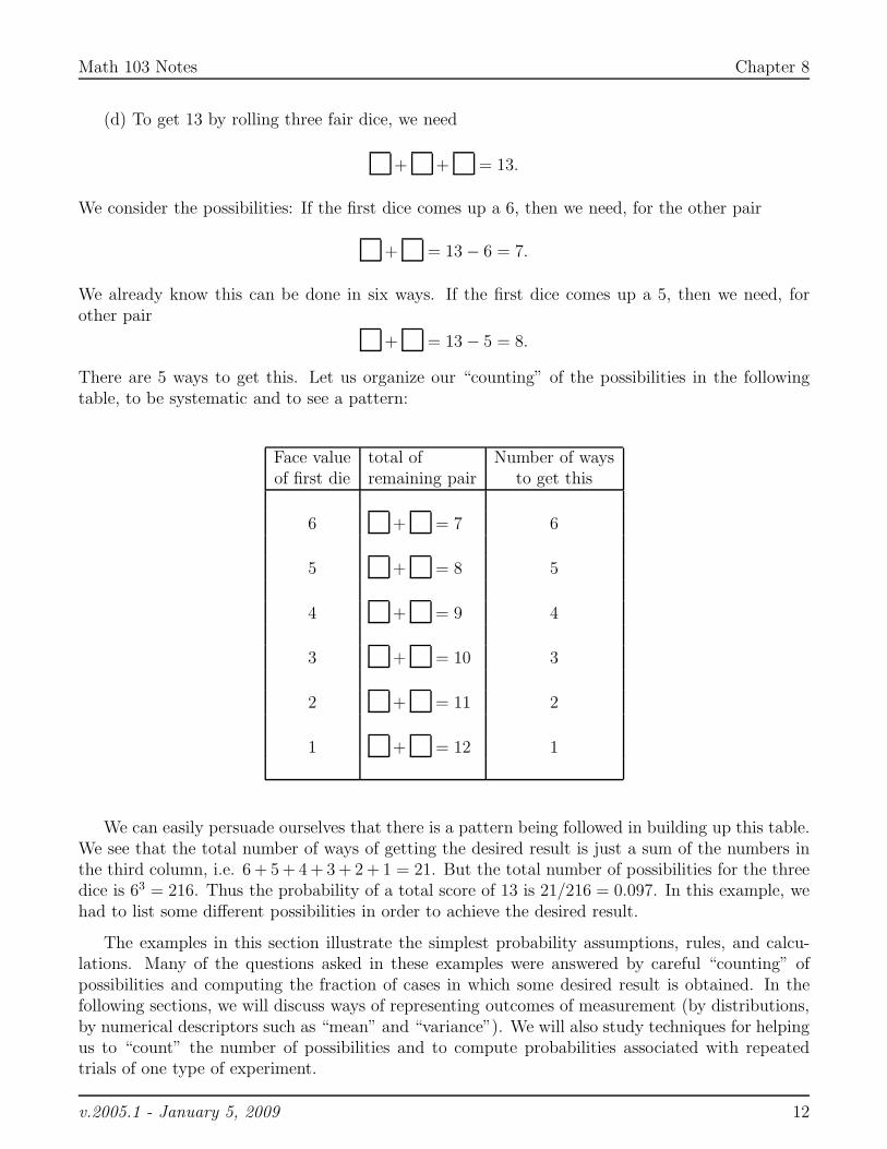
There are 5 ways to get this. Let us organize our “counting” of the possibilities in the followingtable, to be systematic and to see a pattern:
Face value total of Number of waysof first die remaining pair to get this
6 + = 7 6
5 + = 8 5
4 + = 9 4
3 + = 10 3
2 + = 11 2
1 + = 12 1
We can easily persuade ourselves that there is a pattern being followed in building up this table.We see that the total number of ways of getting the desired result is just a sum of the numbers inthe third column, i.e. 6 + 5 + 4 + 3 + 2 + 1 = 21. But the total number of possibilities for the threedice is 63 = 216. Thus the probability of a total score of 13 is 21/216 = 0.097. In this example, wehad to list some different possibilities in order to achieve the desired result.
The examples in this section illustrate the simplest probability assumptions, rules, and calcu-lations. Many of the questions asked in these examples were answered by careful “counting” ofpossibilities and computing the fraction of cases in which some desired result is obtained. In thefollowing sections, we will discuss ways of representing outcomes of measurement (by distributions,by numerical descriptors such as “mean” and “variance”). We will also study techniques for helpingus to “count” the number of possibilities and to compute probabilities associated with repeatedtrials of one type of experiment.
v.2005.1 - January 5, 2009 12
Math 103 Notes Chapter 8
8.8 Theoretical probability of coin tossing
Earlier in this chapter, we studied the results of a coin-tossing experiment. Now we turn to atheoretical investigation of the same type of experiment to understand predictions of the basic rulesof probability. We would like to quantify the probability of getting some number, k, of heads whenthe coin is tossed n times. We start with an elementary example when the coin is tossed only threetimes (N = 3) to build up intuition. Let us use the notation p=P(H) and q=P(T) to represent theprobabilities of each outcome.
For our theoretical probability investigation, we will make the simplest assumption about eachelementary event, i.e. that it is equally likely to obtain a head (H) and tail (T) in one repetition.Then the probabilities of event H and event T in a single toss are the same, i.e. 1/2:
P (H) = P (T ) = 1/2 i.e. p = q = 1/2.
A new feature of this section is that we will summarize the probability using a frequency distri-bution. In this important type of plot, the horizontal axis represents some observed or measuredvalue in an experiment (for example, the number of heads in a coin toss experiment). The verticalaxis represents how often that outcome is obtained (i.e. the frequency, or probability of the event.)
(b) three coin tosses
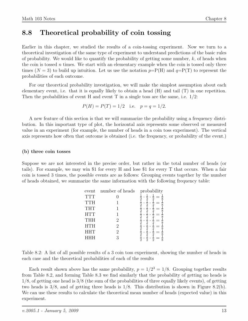
Suppose we are not interested in the precise order, but rather in the total number of heads (ortails). For example, we may win $1 for every H and lose $1 for every T that occurs. When a faircoin is tossed 3 times, the possible events are as follows: Grouping events together by the numberof heads obtained, we summarize the same information with the following frequency table:
event number of heads probabilityTTT 0 1
2· 1
2· 1
2= 1
8
TTH 1 1
2· 1
2· 1
2= 1
8
THT 1 1
2· 1
2· 1
2= 1
8
HTT 1 1
2· 1
2· 1
2= 1
8
THH 2 1
2· 1
2· 1
2= 1
8
HTH 2 1
2· 1
2· 1
2= 1
8
HHT 2 1
2· 1
2· 1
2= 1
8
HHH 3 1
2· 1
2· 1
2= 1
8
Table 8.2: A list of all possible results of a 3 coin toss experiment, showing the number of heads ineach case and the theoretical probabilities of each of the results
Each result shown above has the same probability, p = 1/23 = 1/8. Grouping together resultsfrom Table 8.2, and forming Table 8.3 we find similarly that the probability of getting no heads is1/8, of getting one head is 3/8 (the sum of the probabilities of three equally likely events), of gettingtwo heads is 3/8, and of getting three heads is 1/8. This distribution is shown in Figure 8.2(b).We can use these results to calculate the theoretical mean number of heads (expected value) in thisexperiment.
v.2005.1 - January 5, 2009 13
Math 103 Notes Chapter 8
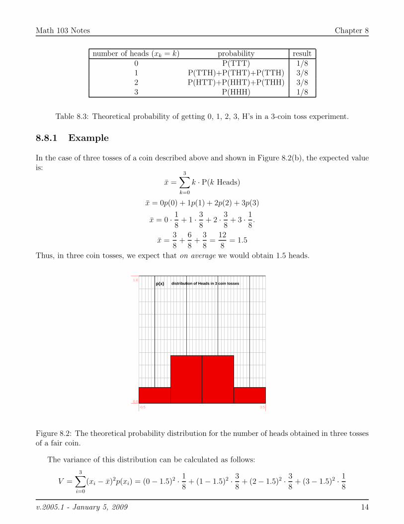
number of heads (xk = k) probability result0 P(TTT) 1/81 P(TTH)+P(THT)+P(TTH) 3/82 P(HTT)+P(HHT)+P(THH) 3/83 P(HHH) 1/8
Table 8.3: Theoretical probability of getting 0, 1, 2, 3, H’s in a 3-coin toss experiment.
8.8.1 Example
In the case of three tosses of a coin described above and shown in Figure 8.2(b), the expected valueis:
x̄ =3
∑
k=0
k · P(k Heads)
x̄ = 0p(0) + 1p(1) + 2p(2) + 3p(3)
x̄ = 0 · 1
8+ 1 · 3
8+ 2 · 3
8+ 3 · 1
8.
x̄ =3
8+
6
8+
3
8=
12
8= 1.5
Thus, in three coin tosses, we expect that on average we would obtain 1.5 heads.
p(x) distribution of Heads in 3 coin tosses
-0.5 3.5
0.0
1.0
Figure 8.2: The theoretical probability distribution for the number of heads obtained in three tossesof a fair coin.
The variance of this distribution can be calculated as follows:
V =
3∑
i=0
(xi − x̄)2p(xi) = (0 − 1.5)2 · 1
8+ (1 − 1.5)2 · 3
8+ (2 − 1.5)2 · 3
8+ (3 − 1.5)2 · 1
8
v.2005.1 - January 5, 2009 14
Math 103 Notes Chapter 8
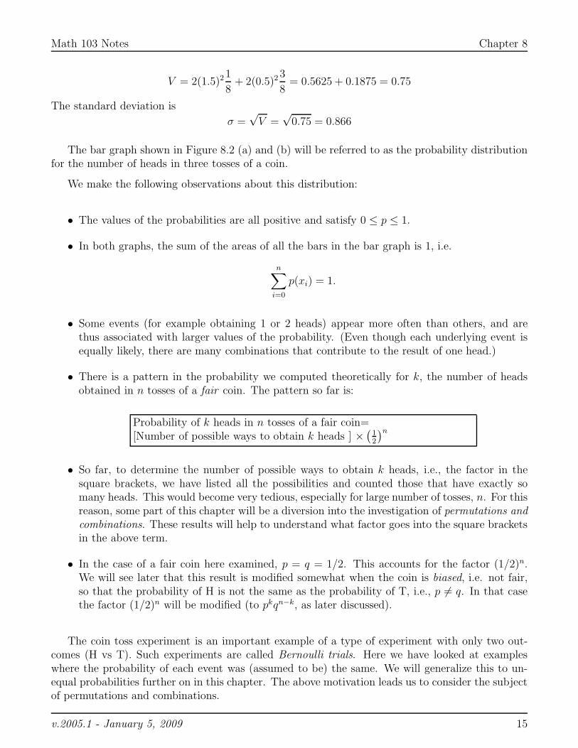
V = 2(1.5)21
8+ 2(0.5)2
3
8= 0.5625 + 0.1875 = 0.75
The standard deviation is
σ =√
V =√
0.75 = 0.866
The bar graph shown in Figure 8.2 (a) and (b) will be referred to as the probability distributionfor the number of heads in three tosses of a coin.
We make the following observations about this distribution:
• The values of the probabilities are all positive and satisfy 0 ≤ p ≤ 1.
• In both graphs, the sum of the areas of all the bars in the bar graph is 1, i.e.
n∑
i=0
p(xi) = 1.
• Some events (for example obtaining 1 or 2 heads) appear more often than others, and arethus associated with larger values of the probability. (Even though each underlying event isequally likely, there are many combinations that contribute to the result of one head.)
• There is a pattern in the probability we computed theoretically for k, the number of headsobtained in n tosses of a fair coin. The pattern so far is:
Probability of k heads in n tosses of a fair coin=[Number of possible ways to obtain k heads ] ×
(
1
2
)n
• So far, to determine the number of possible ways to obtain k heads, i.e., the factor in thesquare brackets, we have listed all the possibilities and counted those that have exactly somany heads. This would become very tedious, especially for large number of tosses, n. For thisreason, some part of this chapter will be a diversion into the investigation of permutations and
combinations. These results will help to understand what factor goes into the square bracketsin the above term.
• In the case of a fair coin here examined, p = q = 1/2. This accounts for the factor (1/2)n.We will see later that this result is modified somewhat when the coin is biased, i.e. not fair,so that the probability of H is not the same as the probability of T, i.e., p 6= q. In that casethe factor (1/2)n will be modified (to pkqn−k, as later discussed).
The coin toss experiment is an important example of a type of experiment with only two out-comes (H vs T). Such experiments are called Bernoulli trials. Here we have looked at exampleswhere the probability of each event was (assumed to be) the same. We will generalize this to un-equal probabilities further on in this chapter. The above motivation leads us to consider the subjectof permutations and combinations.
v.2005.1 - January 5, 2009 15
Math 103 Notes Chapter 8
8.9 How many possible ways are there of getting k heads
in n tosses? permutations and combinations
In computing theoretical probability, we often have to “count” the number of possible ways thereare of obtaining a given type of outcome. So far, it has been relatively easy to simply display allthe possibilities and group them into classes (0, 1, 2, etc heads out of n tosses, etc.). This is notalways the case. When the number of repetitions of an experiment grows, it may be very difficultand boring to list all possibilities. We develop some shortcuts to figure out, in general, how manyways there are of getting each type of outcome. This will make the job of computing theoreticalprobability easier. In this section we introduce some notation and then summarize general featuresof combinations and permutations to help in “counting” the possibilities.
8.9.1 Factorial notation
Let n be an integer, n ≥ 0. Then n!, called “n factorial”, is defined as the following product ofintegers:
n! = n(n − 1)(n − 2) . . . (2)(1)
Example
1! = 1
2! = 2 · 1 = 2
3! = 3 · 2 · 1 = 6
4! = 4 · 3 · 2 · 1 = 24
5! = 5 · 4 · 3 · 2 · 1 = 120
We also define
0! = 1
8.9.2 Permutations
A permutation is a way of arranging objects, where the order of appearance of the objects isimportant.
v.2005.1 - January 5, 2009 16
Math 103 Notes Chapter 8
(c)
n distinct objects n slots
n distinct objects k slots
n distinct objects k objects n n−1 ... n−k+1
n n−1 n−2 ... 2 1
n n−1 ... n−k+1
k slots
n!
(n−k)!
n!P(n,k)=
k!C(n,k)
(a)
(b)
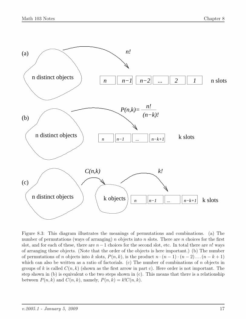
Figure 8.3: This diagram illustrates the meanings of permutations and combinations. (a) Thenumber of permutations (ways of arranging) n objects into n slots. There are n choices for the firstslot, and for each of these, there are n−1 choices for the second slot, etc. In total there are n! waysof arranging these objects. (Note that the order of the objects is here important.) (b) The numberof permutations of n objects into k slots, P (n, k), is the product n · (n − 1) · (n − 2) . . . (n − k + 1)which can also be written as a ratio of factorials. (c) The number of combinations of n objects ingroups of k is called C(n, k) (shown as the first arrow in part c). Here order is not important. Thestep shown in (b) is equivalent o the two steps shown in (c). This means that there is a relationshipbetween P (n, k) and C(n, k), namely, P (n, k) = k!C(n, k).
v.2005.1 - January 5, 2009 17
Math 103 Notes Chapter 8
Example 6
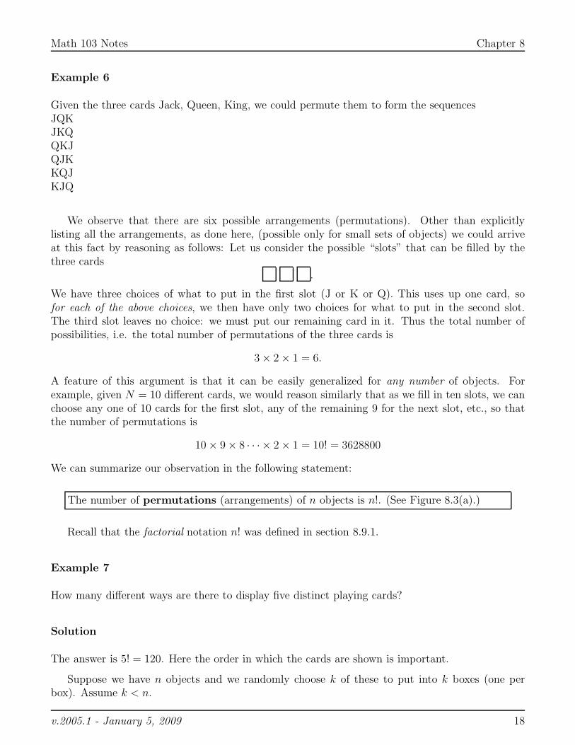
Given the three cards Jack, Queen, King, we could permute them to form the sequencesJQKJKQQKJQJKKQJKJQ
We observe that there are six possible arrangements (permutations). Other than explicitlylisting all the arrangements, as done here, (possible only for small sets of objects) we could arriveat this fact by reasoning as follows: Let us consider the possible “slots” that can be filled by thethree cards
.
We have three choices of what to put in the first slot (J or K or Q). This uses up one card, sofor each of the above choices, we then have only two choices for what to put in the second slot.The third slot leaves no choice: we must put our remaining card in it. Thus the total number ofpossibilities, i.e. the total number of permutations of the three cards is
3 × 2 × 1 = 6.
A feature of this argument is that it can be easily generalized for any number of objects. Forexample, given N = 10 different cards, we would reason similarly that as we fill in ten slots, we canchoose any one of 10 cards for the first slot, any of the remaining 9 for the next slot, etc., so thatthe number of permutations is
10 × 9 × 8 · · · × 2 × 1 = 10! = 3628800
We can summarize our observation in the following statement:
The number of permutations (arrangements) of n objects is n!. (See Figure 8.3(a).)
Recall that the factorial notation n! was defined in section 8.9.1.
Example 7
How many different ways are there to display five distinct playing cards?
Solution
The answer is 5! = 120. Here the order in which the cards are shown is important.
Suppose we have n objects and we randomly choose k of these to put into k boxes (one perbox). Assume k < n.
v.2005.1 - January 5, 2009 18
Math 103 Notes Chapter 8
For example, the objects are
♣♦♥♠ ⋆ • ◦ ⊕
and we must choose some of them (in order) so as to fill up the 4 slots:
We ask ”how many ways there are of arranging n objects taken k at a time?” As in our previousargument, the first slot to fill comes with a choice of n objects (for n possibilities). This “uses up”one object leaving (n − 1) to choose from in the next stage. (For each of the n first choices thereare (n − 1) choices for slot 2, forming the product n · (n − 1)). In the third slot, we have to chooseamong (n − 2) remaining objects, etc. By the time we arrive at the k’th slot, we have (n − k + 1)choices. Thus, in total, the number of ways that we can form such arrangements of n objects intok slots, represented by the notation P (n, k) is
P (n, k) = n · (n − 1) · (n − 2) . . . (n − k + 1).
We can also express this in the form of factorial notation:
P (n, k) =n · (n − 1) · (n − 2) . . . (n − k + 1) · (n − k) · · · · 3 · 2 · 1
(n − k) . . . (n − k − 1) · · · · 3 · 2 · 1 =n!
(n − k)!.
These remarks motivate the following observation:
The number of permutations of n objects taken k at a time is
P (n, k) =n!
(n − k)!.
(See Figure 8.3(b).)
8.9.3 Combinations and binomial coefficients
How many ways are there to choose k objects out of a set of n objects if the order of the selectiondoes not matter? For example, if we have a class of 10 students, how many possible pairs of studentscan be formed for a team project? In the case that the order of the objects is not important, werefer to the number of possible combinations of n objects taken k at a time by the notation C(n, k)or, more commonly, by
C(n, k) =
(
nk
)
=n!
(n − k)!k!
Note that two notations are commonly used to refer to the same concept. We will henceforth usemainly the notation C(n, k). We can read this notation as “n choose k”. The values C(n, k) arealso called the binomial coefficients for reasons that will shortly become apparent.
As shown in Figure 8.3(b,c), combinations are related to permutations in the following way: Tofind the number of permutations of n objects taken k at a time, P (n, k), we would
v.2005.1 - January 5, 2009 19
Math 103 Notes Chapter 8
• Choose k out of n objects. But the number of ways of doing this is C(n, k), i.e.,
C(n, k) =
(
nk
)
• Find all the permutations of the k chosen objects. We have discussed that there are k! waysof arranging (i.e. permuting) k objects.
Thus
P (n, k) =
(
nk
)
· k!
The above remarks lead to the following conclusion:
The number of combinations of n objects taken k at a time, sometimes called “n choosek”, (also called the binomial coefficient, C(n, k)) is:
C(n, k) =
(
nk
)
=P (n, k)
k!=
n!
k!(n − k)!.
We can observe an interesting symmetry property, namely that(
nk
)
=
(
nn − k
)
or C(n, k) = C(n, n − k).
It is worth noting that the binomial coefficients are entries that occur in Pascal’s triangle:
1
1 1
1 2 1
1 3 3 1
1 4 6 4 1
1 5 10 10 5 1
Each term in Pascal’s triangle is obtained by adding the two diagonally above it. The top of thetriangle represents C(0, 0) and is associated with n = 0. The next row represents C(1, 0) andC(1, 1). For row number n, terms along the row are the binomial coefficients C(n, k), starting withk = 0 at the beginning of the row and and going to k = n at the end of the row. For example,we see above that the value of C(5, 2) = C(5, 3) = 10 The triangle can be continued, by includingsubsequent rows; this is left as an exercise for the reader.
8.9.4 Example
How many ways are there of getting k heads in n tosses of a fair coin?
v.2005.1 - January 5, 2009 20
Math 103 Notes Chapter 8
Solution
This problem motivated the discussion of permutations and combinations. We can now answer thisquestion.
The number of possible ways of obtaining k heads in n tosses is
C(n, k) =n!
k!(n − k)!.
Thus the probability of getting any outcome consisting of k heads when a fair coin is tossed n times,is
For a fair coin, P(k heads in n tosses)=n!
k!(n − k)!
(
1
2
)n
.
The term containing the power (1/2)n is the probability of any one specific sequence of possibleH’s and T’s. The multiplier in front, which as we have seen is the binomial coefficient C(n, k), ishow many such sequences have exactly k H’s and all the rest (i.e., n − k) T’s. (The greater thenumber of possible combinations, the more likely it is that any one of them would occur.)
8.9.5 Example
How many combinations can be made out of of 5 objects if we take 1, or 2 or 3 etc objects at atime?
Solution
Here the order of the objects is not important. The number of ways of taking 5 objects k at a time(where 0 ≤ k ≤ 5) is C(5, k). For example, the number of combinations of 5 objects taken 3 at atime is
C(5, 3) =5!
3!(5 − 3)!=
5 · 4 · 3 · 2 · 1(3 · 2 · 1)(2 · 1)
=5 · 42
= 10.
The list of all the coefficients C(5, k) appears as the last row displayed above in Pascal’s triangle.
8.9.6 Example
How many different 5-card hands can be formed from a deck of 52 ordinary playing cards?
v.2005.1 - January 5, 2009 21
Math 103 Notes Chapter 8
Solution
We are not concerned here with the order of appearance of the cards that are dealt, only withthe “hand” (i.e. composition of the final collection of 5 cards). Thus we are asking how manycombinations of 5 cards there are from a set of 52 cards. The solution is
C(52, 5) =52!
5!(52 − 5)!=
52 · 51 · 50 · 49 · 48
5 · 4 · 3 · 2 · 1 = 2, 598, 960.
8.9.7 The binomial theorem
An interesting application of combinations is the formula for the product of terms of the form(a + b)n known as the Binomial expansion. Consider the simple example
(a + b)2 = (a + b) · (a + b).
We expand this by multiplying each of the terms in the first factor by each of the terms in thesecond factor:
(a + b)2 = a2 + ab + ba + b2.
However, the order of factors ab or ba does not matter, so we count these as two identical terms,and express our result as
(a + b)2 = a2 + 2ab + b2.
Similarly, consider the product
(a + b)3 = (a + b)(a + b)(a + b).
Now, to form the expansion, each term in the first factor is multiplied by two other terms (onechosen from each of the other factors). This leads to an expansion of the form
(a + b)3 = a3 + 3a2b + 3ab2 + b3.
More generally, consider a product of the form
(a + b)n = (a + b) · (a + b) · · · · (a + b).
By analogy, we expect to see terms of the form shown below in the expansion for this binomial, i.e.
(a + b)n = an + an−1b + an−2b2 + · · · + an−kbk + · · · + abn−1 + bn.
The first and last terms are accompanied by the “coefficients” 1, since such terms can occur in onlyone way each. However, we must still “fill in the boxes” with coefficients that reflect the number oftimes that terms of the given form an−kbk occur. But this product is made by choosing k a’s out ofa total of n factors (and picking b’s from all the rest of the factors). We already know how manyways there are of selecting k items out of a collection of n, namely, the binomial coefficients. Thus
(a+b)n = an+C(n, 1)an−1b+C(n, 2)an−2b2+· · ·+C(n, k)akbn−k+· · ·+C(n, 2)a2bn−2+C(n, 1)abn−1+bn
where the binomial coefficients are as defined in section 8.9.3. We have used the symmetry propertyC(n, k) = C(n, n − k) in the coefficients in this expansion.
v.2005.1 - January 5, 2009 22
Math 103 Notes Chapter 8
8.9.8 Example
Find the expansion of the expression (a + b)5.
Solution
The coefficients we need in this expansion are formed from C(5, k). We have already calculated thebinomial coefficients for the required expansion in example 8.9.5, namely, 1 5 10 10 5 1. Thus thedesired expansion is
(a + b)5 = a5 + 5a4b + 10a3b2 + 10a2b3 + 5ab4 + b5.
8.10 A coin toss experiment and binomial distribution
A Bernoulli Trial is an experiment that has only two possible results. A typical example of this typeis the coin toss. We have already studied examples of results of a Bernoulli trial in this chapter.Here we expand our investigation to consider more general cases and their distributions.
We have already examined in detail an example of a Bernoulli trial in which each outcome isequally likely, i.e. a coin toss with P(H) = P(T). In this section we will drop the assumption thateach event is equally likely, and examine a more general case.
If we do not know that the coin is fair, we might assume that the probability that it lands on His p and on T is q. That is
p(H) = p, p(T ) = q
In general, p and q may not be exactly equal. By the property of probabilities,
p + q = 1
Consider the following specific outcome of an experiment in which an (unfair) coin is tossed 10times:TTHTHHTTTHAssuming that each toss is independent of the other tosses, we find that the probability of thisevent is: q · q · p · q · p · p · q · q · q · p = p4q6. The probability of this specific event is the sameas the probability of the specific event HHHHTTTTTT (Since each event has the same number ofH’s and T’s). The probability of each event is a product of factors of p and q (one for each of Hor T that appear). Further, the number of ways of obtaining an outcome with a specific numberof H’s (for example, four H’s as in this illustration) is the same whether the coin is fair or not.(That number is a combination, i.e. the binomial coefficient C(n, k) as before.) The probability ofgetting any outcome with k heads when the (possibly unfair) coin is tossed n times is thus a simplegeneralization of the probability for a fair coin:
v.2005.1 - January 5, 2009 23
Math 103 Notes Chapter 8
The binomial distribution
Given a (possibly unfair) coin with P(H)= p, and P(T)=q, where p + q = 1, if the coin istossed n times, the probability of getting exactly k heads is given by
P (k heads out of n tosses) = C(n, k)pkqn−k =n!
k!(n − k)!pkqn−k.
We refer to this distribution as the Binomial distribution. In the case of a fair coin,p = q = 1/2 and the factor pkqn−k is replaced by (1/2)n.
Having obtained the form of the binomial distribution, we wish to show that the probability ofobtaining any of the possible outcomes, i.e. P(1 or 2 or . . . n Heads out of n tosses)=1. We canshow this with the following calculation.
For each toss,(p + q) = 1.
Then raising each side to the power n,
(p + q)n = 1n = 1,
but by the Binomial theorem, the expression on the left can be expanded, to form,
(p+q)n = pn+C(n, 1)pn−1q+C(n, 2)pn−2q2+· · ·+C(n, k)pkqn−k+· · ·+C(n, 2)p2qn−2+C(n, 1)pqn−1+qn,
that is,
(p + q)n =n
∑
k=0
C(n, k)pkqn−k
Therefore, since (p + q)n = 1, it follows that
n∑
k=0
C(n, k)pkqn−k = 1
Thus∑n
k=0P(k Heads out of n tosses)=1, verifying the desired relationship.
Remark: Each term in the above expansion can be interpreted as the probability of a certaintype of event. The first term is the probability of tossing exactly n heads: there is only one way thiscan happen, accounting for the coefficient 1. The last term is the probability of tossing exactly nTails. The product pkqn−k reflects the probability of a particular sequence containing k Heads andthe rest (n − k) Tails: but there are many ways of generating that type of sequence: C(n, k) is thenumber of distinct combinations that are all counted as k heads. Thus the combined probability ofgetting any of the events in which there are k Heads is given by C(n, k)pkqn−k.
8.10.1 Example
Suppose P(H)=p = 0.1. What is the probability of getting 3 Heads if this unfair coin is tossed 5times?
v.2005.1 - January 5, 2009 24
Math 103 Notes Chapter 8
Solution
¿From the above results, P (3 heads out of 5 tosses) = p3q2C(5, 3). But p = 0.1 and q = 1−p =0.9, so P(3 heads out of 5 tosses)= 0.130.92C(5, 3) = (0.001)(.81)10 = 0.0081
8.11 Mean of a binomial distribution
A binomial distribution has a particularly simple mean. An important result, established in thecalculations in this section is as follows:
Consider a Bernoulli trial in which the probability of event e1 is p. Then if this trial isrepeated n times, the mean of the resulting binomial distribution, i.e. expected number oftimes that event e1 occurs is
x̄ = np.
Thus the mean of a binomial distribution is the number of repetitions multiplied by theprobability of the event in a single trial.
We here verify the simple formula for the mean of a binomial distribution. The calculationsuse many properties of series that were established in Chapter 1. The calculation is presented forcompleteness, rather than importance but the result (in the box above) is very useful and important.
By definition of the mean,
x̄ =n
∑
k=0
xkp(xk)
But here xk = k is the number of heads obtained, and p(xk)=P(k heads in n tosses)= C(n, k)pkqn−k
is the distribution of k heads in n tosses computed in this chapter. Then
x̄ =n
∑
k=0
k · C(n, k)pkqn−k =n
∑
k=1
kn!
k!(n − k)!pkqn−k
where in the last sum we have dropped the k = 0 term, since it makes no contribution to the total.The numerators in the sum are of the form k · n · (n − 1) . . . (n − k + 1) and the denominators arek · (k − 1) . . . 2 · 1. We can cancel one factor of k from top and bottom. We can also take onecommon factor of n out of the sum:
x̄ =n
∑
k=1
n(n − 1) . . . (n − k + 1)
(k − 1) . . . 2 · 1 pkqn−k = nn
∑
k=1
(n − 1) . . . (n − k + 1)
(k − 1) . . . 2 · 1 pkqn−k
We now shift the sum by defining the following replacement index: let ℓ = k − 1 then k = ℓ + 1 sowhen k = 1, ℓ = 0 and when k = n, ℓ = n − 1. We replace the indices and take one common factorof p out of the sum:
x̄ = n
n−1∑
ℓ=0
(n − 1) . . . (n − ℓ)
ℓ!pℓ+1qn−ℓ−1 = np
n−1∑
ℓ=0
(n − 1)!
ℓ!(n − ℓ − 1)!pℓqn−ℓ−1
v.2005.1 - January 5, 2009 25
Math 103 Notes Chapter 8
Let m = n − 1, then
x̄ = np
m∑
ℓ=0
m!
ℓ!(n − m)!pℓqm−ℓ = np,
where in the last step we have used the fact that∑n
k=0p(xk) = 1. This verifies the result.
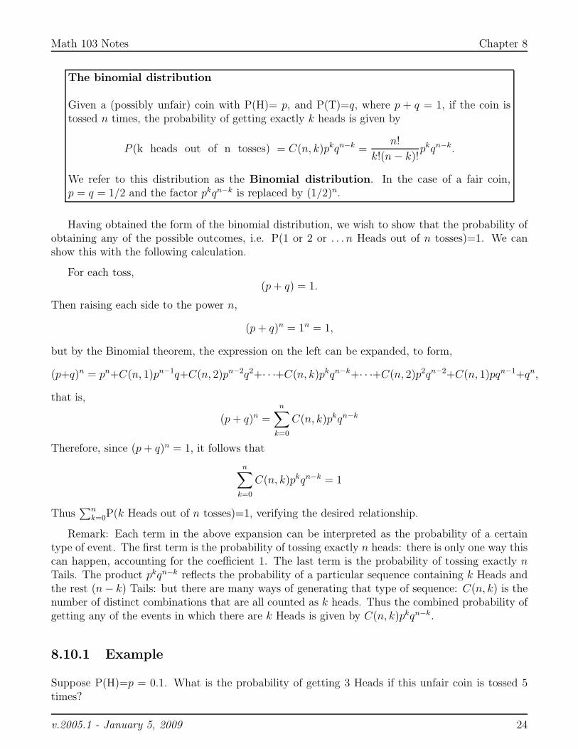
8.12 A continuous distribution
The Normal distribution
-4.0 4.0
0.0
0.4
Figure 8.4: The Normal (or Gaussian) distribution is given by equation (8.1) and has the distributionshown in this figure.
If we were to repeat the number of coin tosses a large number of times, n, we would see a certaintrend: There would be a peak in the distribution at the probability of getting heads 50% of thetime, i.e. at N/2 heads.
A fact which we state but do not prove here is that the probability of N/2 heads, p(N/2) behaveslike
p(N/2) ≈√
2
πN=
√
1
2π
√
4
N.
This can also be written in the form√
N
4p(N/2) ≈
√
1
2π= Const.
v.2005.1 - January 5, 2009 26
Math 103 Notes Chapter 8
One finds that the shapes of the various distributions is similar, but that a scale factor of√
N/2 isapplied to stretch the graph horizontally, while compressing it vertically to preserve its total area.The graph is also shifted so that its peak occurs at N/2.
As the number of Bernoulli trials grows, i.e. as we toss our imaginary coin in longer and longersets (N → ∞), a remarkable thing happens to the binomial distribution: it becomes smootherand smoother, until it grows to resemble a continuous distribution that looks like a “Bell curve”.That curve is known as the Gaussian or Normal distribution. If we scale this curve vertically andhorizontally (stretch vertically and compress horizontally by the factor
√N/2) and shift its peak
to x = 0, then we find a distribution that describes the deviation from the expected value of 50%heads. The resulting function is of the form
p(x) =1√2π
e−x2/2 (8.1)
We will study properties of this (and other) such continuous distributions in a later section. Weshow a typical example of the Normal distribution in Figure 8.4. Its cumulative distribution is thenshown (without and with the original distribution superimposed) in Figure 8.5.
The cumulative distribution
-4.0 4.0
0.0
1.0
The cumulative distribution
The normal distribution
-4.0 4.0
0.0
1.0
Figure 8.5: The Normal probability density with its corresponding cumulative distribution.
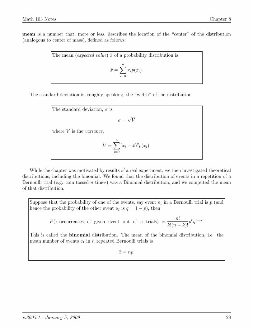
8.13 Summary
In this chapter, we introduced the notion of probability of elementary events. We learned that aprobability is always a number between 0 and 1, and that the sum of (discrete) probabilities of allpossible (discrete) outcomes is 1. We then described how to combine probabilities of elementaryevents to calculate probabilities of compound independent events in a variety of simple experiments.We defined the notion of a Bernoulli trial, such as tossing of a coin, and studied this in detail.
We investigated a number of ways of describing results of experiments, whether in tabular orgraphical form, and we used the distribution of results to define simple numerical descriptors. The
v.2005.1 - January 5, 2009 27
Math 103 Notes Chapter 8
mean is a number that, more or less, describes the location of the “center” of the distribution(analogous to center of mass), defined as follows:
The mean (expected value) x̄ of a probability distribution is
x̄ =n
∑
i=0
xip(xi).
The standard deviation is, roughly speaking, the “width” of the distribution.
The standard deviation, σ is
σ =√
V
where V is the variance,
V =n
∑
i=0
(xi − x̄)2p(xi).
While the chapter was motivated by results of a real experiment, we then investigated theoreticaldistributions, including the binomial. We found that the distribution of events in a repetition of aBernoulli trial (e.g. coin tossed n times) was a Binomial distribution, and we computed the meanof that distribution.
Suppose that the probability of one of the events, say event e1 in a Bernoulli trial is p (andhence the probability of the other event e2 is q = 1 − p), then
P (k occurrences of given event out of n trials) =n!
k!(n − k)!pkqn−k.
This is called the binomial distribution. The mean of the binomial distribution, i.e. themean number of events e1 in n repeated Bernoulli trials is
x̄ = np.
v.2005.1 - January 5, 2009 28