Chapter 7 Water Flow in Open Channels

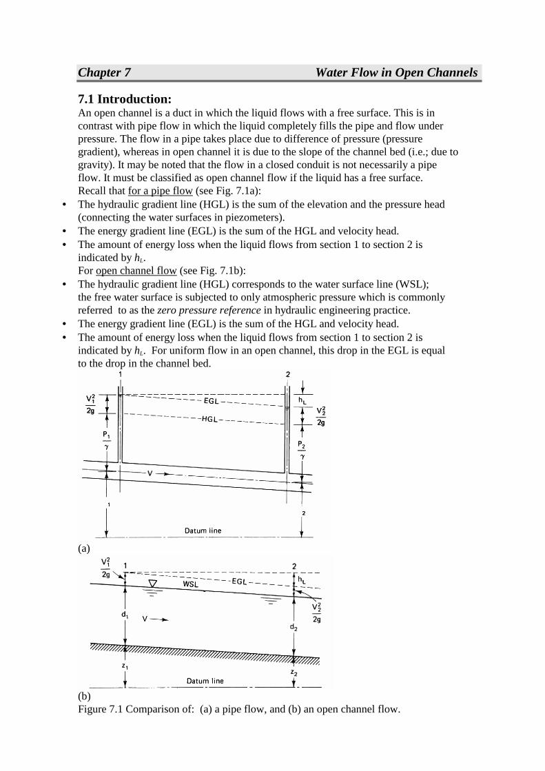
7.1 Introduction: An open channel is a duct in which the liquid flows with a free surface. This is in contrast with pipe flow in which the liquid completely fills the pipe and flow under pressure. The flow in a pipe takes place due to difference of pressure (pressure gradient), whereas in open channel it is due to the slope of the channel bed (i.e.; due to gravity). It may be noted that the flow in a closed conduit is not necessarily a pipe flow. It must be classified as open channel flow if the liquid has a free surface. Recall that for a pipe flow (see Fig. 7.1a):

• The hydraulic gradient line (HGL) is the sum of the elevation and the pressure head (connecting the water surfaces in piezometers).

• The energy gradient line (EGL) is the sum of the HGL and velocity head. • The amount of energy loss when the liquid flows from section 1 to section 2 is

indicated by hL. For open channel flow (see Fig. 7.1b):

• The hydraulic gradient line (HGL) corresponds to the water surface line (WSL); the free water surface is subjected to only atmospheric pressure which is commonly referred to as the zero pressure reference in hydraulic engineering practice.

• The energy gradient line (EGL) is the sum of the HGL and velocity head. • The amount of energy loss when the liquid flows from section 1 to section 2 is

indicated by hL. For uniform flow in an open channel, this drop in the EGL is equal to the drop in the channel bed.

(a)

(b) Figure 7.1 Comparison of: (a) a pipe flow, and (b) an open channel flow.

7.2 Type of Open Channels: Based on their existence, an open channel can be natural or artificial:

One)Natural channels such as streams, rivers, valleys , etc. These are generally irregular in shape, alignment and roughness of the surface.

Two)Artificial channels are built for some specific purpose, such as irrigation, water supply, wastewater, water power development, and rain collection channels. These are regular in shape and alignment with uniform roughness of the boundary surface. Based on their shape, an open channel can be prismatic or non-prismatic:

One)Prismatic channels: a channel is said to be prismatic when the cross section is uniform and the bed slop is constant.

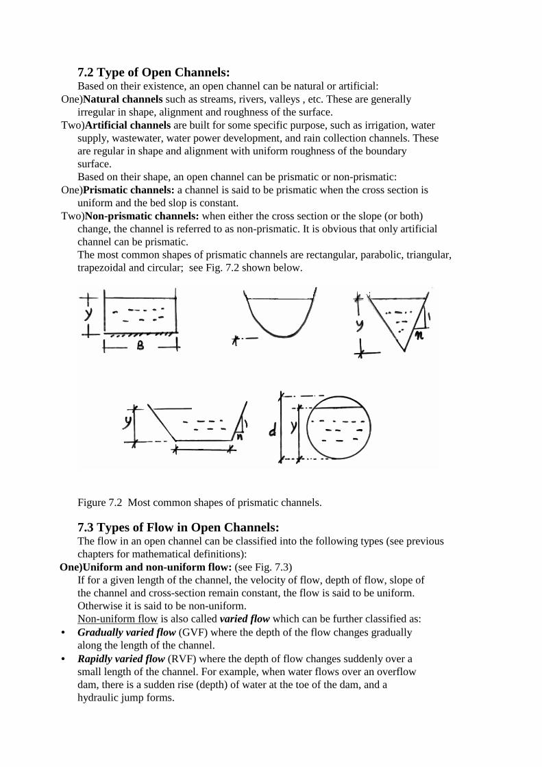
Two)Non-prismatic channels: when either the cross section or the slope (or both) change, the channel is referred to as non-prismatic. It is obvious that only artificial channel can be prismatic. The most common shapes of prismatic channels are rectangular, parabolic, triangular, trapezoidal and circular; see Fig. 7.2 shown below.

Figure 7.2 Most common shapes of prismatic channels.

7.3 Types of Flow in Open Channels: The flow in an open channel can be classified into the following types (see previous chapters for mathematical definitions):

One)Uniform and non-uniform flow: (see Fig. 7.3) If for a given length of the channel, the velocity of flow, depth of flow, slope of the channel and cross-section remain constant, the flow is said to be uniform. Otherwise it is said to be non-uniform. Non-uniform flow is also called varied flow which can be further classified as:

• Gradually varied flow (GVF) where the depth of the flow changes gradually along the length of the channel.

• Rapidly varied flow (RVF) where the depth of flow changes suddenly over a small length of the channel. For example, when water flows over an overflow dam, there is a sudden rise (depth) of water at the toe of the dam, and a hydraulic jump forms.

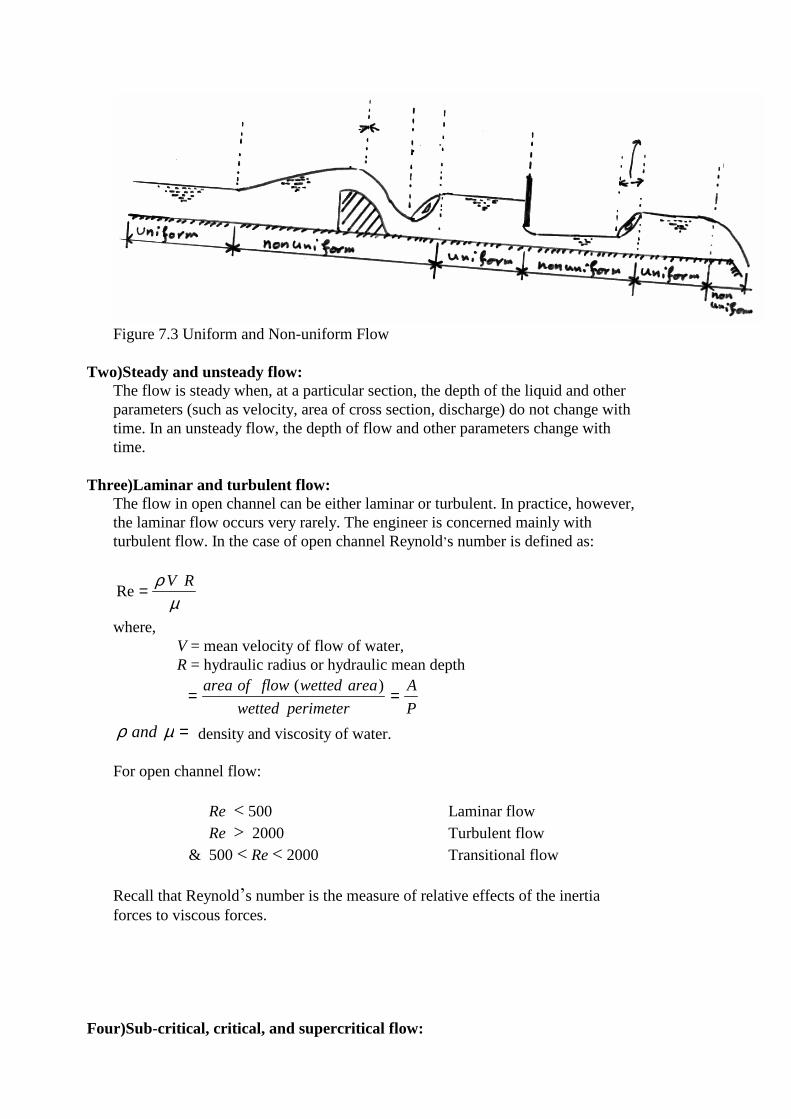
Figure 7.3 Uniform and Non-uniform Flow

Two)Steady and unsteady flow: The flow is steady when, at a particular section, the depth of the liquid and other parameters (such as velocity, area of cross section, discharge) do not change with time. In an unsteady flow, the depth of flow and other parameters change with time.

Three)Laminar and turbulent flow: The flow in open channel can be either laminar or turbulent. In practice, however, the laminar flow occurs very rarely. The engineer is concerned mainly with turbulent flow. In the case of open channel Reynold’s number is defined as:

Re=ρ

µV R

where, V = mean velocity of flow of water, R = hydraulic radius or hydraulic mean depth

= =area of flow wetted area

wetted perimeter

A

P

( )

ρ µand = density and viscosity of water. For open channel flow: Re < 500 Laminar flow Re > 2000 Turbulent flow & 500 < Re < 2000 Transitional flow Recall that Reynold’s number is the measure of relative effects of the inertia forces to viscous forces.

Four)Sub-critical, critical, and supercritical flow:

The criterion used in this classification is what is known by Froude number, Fr, which is the measure of the relative effects of inertia forces to gravity force:

FrV

g Dh

=

where, V = mean velocity of flow of water, Dh = hydraulic depth of the channel

= =area of flow wetted area

water surface width

A

T

( )

For open channel flow: Fr < 1 Sub-critical flow Fr = 1 Critical flow & Fr > 1 Supercritical flow 7.4 Flow Formulas in Open Channels (steady-uniform flow): In the case of steady-uniform flow in an open channel, the following main features must be satisfied:

• The water depth, water area, discharge, and the velocity distribution at all sections throughout the entire channel length must remain constant, i.e.; Q , A , y , V remain constant through the channel length.

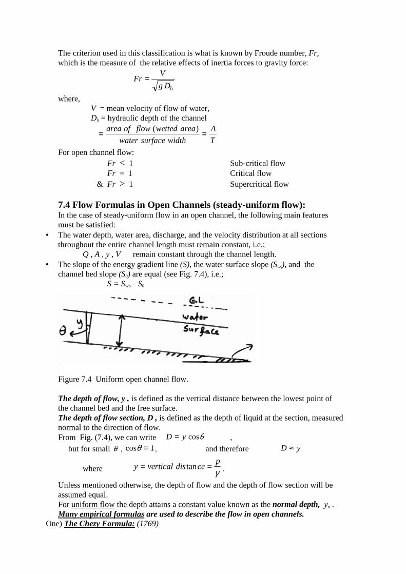
• The slope of the energy gradient line (S), the water surface slope (Sws), and the channel bed slope (S0) are equal (see Fig. 7.4), i.e.; S = Sws = S0

Figure 7.4 Uniform open channel flow. The depth of flow, y , is defined as the vertical distance between the lowest point of the channel bed and the free surface. The depth of flow section, D , is defined as the depth of liquid at the section, measured normal to the direction of flow. From Fig. (7.4), we can write D y= cosθ ,

but for small θ , cosθ = 1, and therefore D y≈

where y vertical dis cep

= =tanγ .

Unless mentioned otherwise, the depth of flow and the depth of flow section will be assumed equal. For uniform flow the depth attains a constant value known as the normal depth, yn . Many empirical formulas are used to describe the flow in open channels.

One) The Chezy Formula: (1769)

The Chezy formula is probably the first formula derived for uniform flow. It may be expressed in the following form:

V C R Sh= (7.1)

where C = Chezy coefficient (Chezy’s resistance factor), m1/2/s.

Two) The Manning Formula: (1895) Using the analysis performed on his own experimental data and on those of others, Manning derived the following empirical relation:

Cn

Rh=1 1 6/

(7.2)

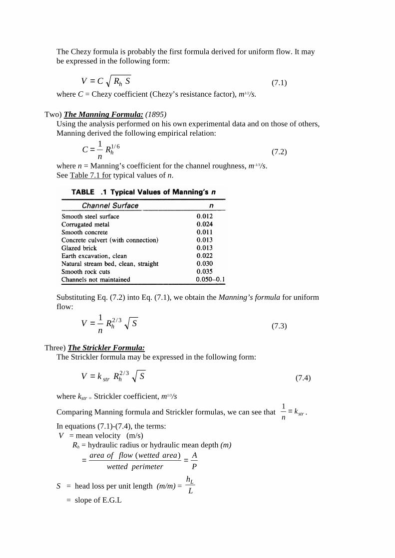
where n = Manning’s coefficient for the channel roughness, m-1/3/s. See Table 7.1 for typical values of n.

Substituting Eq. (7.2) into Eq. (7.1), we obtain the Manning’s formula for uniform flow:

Vn

R Sh=1 2 3/

(7.3)

Three) The Strickler Formula:

The Strickler formula may be expressed in the following form:

V k R Sstr h= 2 3/ (7.4)

where kstr = Strickler coefficient, m1/3/s

Comparing Manning formula and Strickler formulas, we can see that 1

nkstr= .

In equations (7.1)-(7.4), the terms: V = mean velocity (m/s) Rh = hydraulic radius or hydraulic mean depth (m)

= =area of flow wetted area

wetted perimeter

A

P

( )

S = head loss per unit length (m/m) = h

LL

= slope of E.G.L

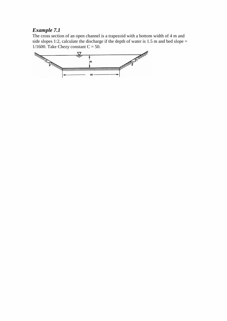
Example 7.1 The cross section of an open channel is a trapezoid with a bottom width of 4 m and side slopes 1:2, calculate the discharge if the depth of water is 1.5 m and bed slope = 1/1600. Take Chezy constant C = 50.

7.5 Most Economical Section of Channels: A section of a channel is said to be most economical when the cost of construction of the channel is minimum. But the cost of construction of a channel depends on excavation and the lining. To keep the cost down or minimum, the wetted perimeter, for a given discharge, should be minimum. This condition is utilized for determining the dimensions of economical sections of different forms of channels. Most economical section is also called the best section or most efficient section as the discharge, passing through a most economical section of channel for a given cross-sectional area A, slope of the bed S0 and a resistance coefficient, is maximum. But the discharge

Q AV A C R S A CA

PS const

Ph= = = = .*

1

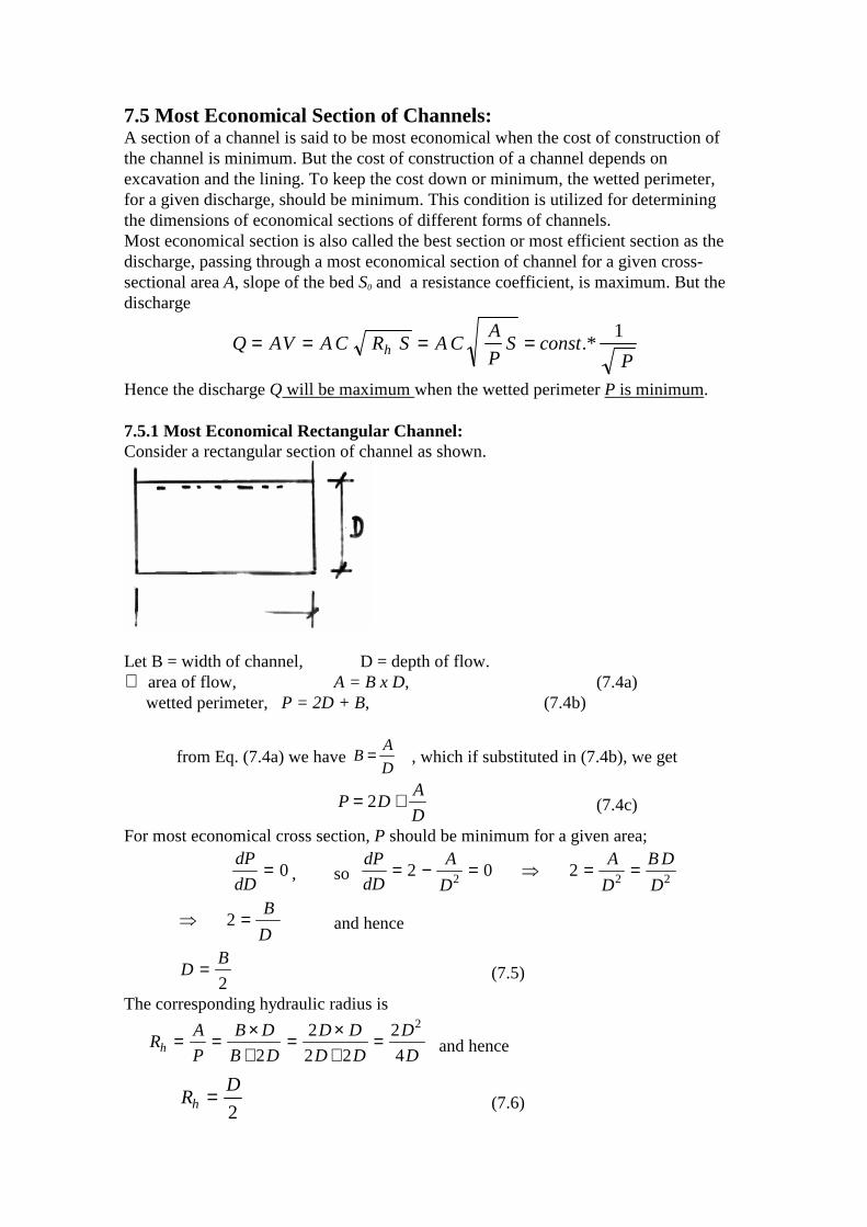
Hence the discharge Q will be maximum when the wetted perimeter P is minimum. 7.5.1 Most Economical Rectangular Channel: Consider a rectangular section of channel as shown.

Let B = width of channel, D = depth of flow. ∴ area of flow, A = B x D, (7.4a) wetted perimeter, P = 2D + B, (7.4b)

from Eq. (7.4a) we have BA

D= , which if substituted in (7.4b), we get

P DA

D= +2 (7.4c)

For most economical cross section, P should be minimum for a given area;

dP

dD= 0 , so

dP

dD

A

D

A

D

B D

D= − = ⇒ = =2 0 2

2 2 2

⇒ =2B

D and hence

DB

=2

(7.5)

The corresponding hydraulic radius is

RA

P

B D

B D

D D

D D

D

Dh = =×

+=

×+

=2

2

2 2

2

4

2

and hence

RD

h =2 (7.6)

From equations (7.5) and (7.6), it is clear that rectangular channel will be most economical when either:

(a) the depth of the flow is half the width (Eq. 7.5), or (b) the hydraulic radius is half the depth of flow (eq. 7.6).

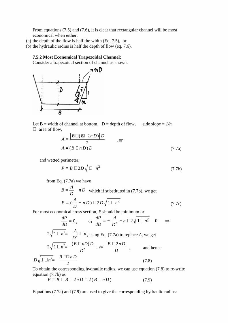
7.5.2 Most Economical Trapezoidal Channel: Consider a trapezoidal section of channel as shown.

Let B = width of channel at bottom, D = depth of flow, side slope = 1/n ∴ area of flow,

[ ]

AB B n D D

=+ +( )2

2 , or

A B n D D= +( ) (7.7a) and wetted perimeter,

P B D n= + +2 1 2 (7.7b)

from Eq. (7.7a) we have

BA

Dn D= − which if substituted in (7.7b), we get

PA

Dn D D n= − + +( ) 2 1 2

(7.7c)

For most economical cross section, P should be minimum or

dP

dD= 0 , so

dP

dD

A

Dn n= − − + + = ⇒

222 1 0

2 1 22

+ = +nA

Dn , using Eq. (7.7a) to replace A, we get

2 122

2+ =+

+ =+

nB nD D

Dn

B n D

D

( ) , and hence

D nB n D

12

22+ =

+ (7.8)

To obtain the corresponding hydraulic radius, we can use equation (7.8) to re-write equation (7.7b) as

P B B n D B n D= + + = +2 2 ( ) (7.9) Equations (7.7a) and (7.9) are used to give the corresponding hydraulic radius:

RA

P

B n D D

B n Dh = =+

+( )

( )2 and hence

RD

h =2 (7.10)

From equations (7.8) and (7.10), it is clear that trapezoidal channel will be most economical when either: (i) one of the sloping sides (wetted length) = half of the top width (Eq. 7.8), or (ii) the hydraulic radius is half the depth of flow (Eq. 7.10).

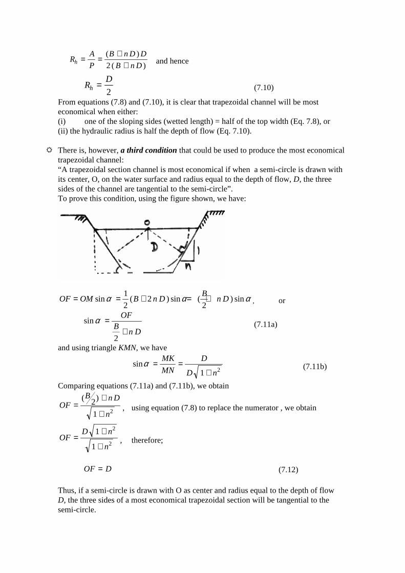
� There is, however, a third condition that could be used to produce the most economical trapezoidal channel: “A trapezoidal section channel is most economical if when a semi-circle is drawn with its center, O, on the water surface and radius equal to the depth of flow, D, the three sides of the channel are tangential to the semi-circle”. To prove this condition, using the figure shown, we have:

OF OM B n DB

n D= = + = +sin ( ) sin ( ) sinα α α1

22

2, or

sinα =+

OFB

n D2

(7.11a)

and using triangle KMN, we have

sinα = =+

MK

MN

D

D n1 2 (7.11b)

Comparing equations (7.11a) and (7.11b), we obtain

OFB n D

n=

+

+

( )2

1 2 , using equation (7.8) to replace the numerator , we obtain

OFD n

n=

+

+

1

1

2

2 , therefore;

OF D= (7.12)

Thus, if a semi-circle is drawn with O as center and radius equal to the depth of flow D, the three sides of a most economical trapezoidal section will be tangential to the semi-circle.

� Best side slope for most economical trapezoidal section can be shown to be when

n =1

3:

So far we assumed that the side slopes are constant. Let us now consider the case when the side slopes can also vary. The most economical side slopes of a most economical trapezoidal section can be obtained as follows: Equation (7.8) can be re-written as

B D n n= + −2 1 2( ) (7.13a)

and from Eq. (7.7a) we have

BA

Dn D= − (7.13b)

equating the above two equations, we get A

Dn D D n n− = + −2 1 2( ) from which we find

DA

n n

2

22 1=

+ − (7.14)

Now, from equation (7.9),P B n D= +2( ) , and equation (7.13b), we can write

PA

D= 2 , squaring both sides and use equation (7.14), we get

PA

DA n n2 2 24 4 2 1= = + −( ) ( ) ,

for most economical side slopes of a most efficient cross section we satisfy the

condition dP

dn= 0 , i.e.;

2 4 1 2 121

2PdP

dnA n n= + −

−[( ) * ( ) ] and applying the condition we get

2

11

2

n

n+= , simplifying we get

4 12 2n n= + , and hence

n =1

3 or

1 3

1n= = tanθ ⇒ =θ ο60

Therefore, best side slope is at 60o to the horizontal, i.e.; of all trapezoidal sections a half hexagon is most economical. However, because of constructional difficulties, it may not be practical to adopt the most economical side slopes. 7.5.3 Most Economical Circular Channel:

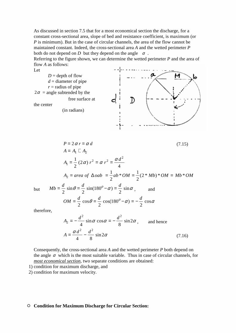
As discussed in section 7.5 that for a most economical section the discharge, for a constant cross-sectional area, slope of bed and resistance coefficient, is maximum (or P is minimum). But in the case of circular channels, the area of the flow cannot be maintained constant. Indeed, the cross-sectional area A and the wetted perimeter P both do not depend on D but they depend on the angle α . Referring to the figure shown, we can determine the wetted perimeter P and the area of flow A as follows: Let D = depth of flow d = diameter of pipe r = radius of pipe 2α = angle subtended by the free surface at the center (in radians) P r d= =2α α (7.15)

A A A= +1 2

A r rd

12 2

21

22

4= = =( )α α α

A area of oab ab OM Mb OM Mb OM21

2

1

22= = = =∆ * ( * ) * *

but Mbd d d= = − =2 2

1802

sin sin( ) sinθ α αο, and

OMd d d= = − = −2 2

1802

cos cos( ) cosθ α αο

therefore,

Ad d

2

2 2

4 82= − = −sin cos sinα α α , and hence

Ad d

= −α α

2 2

4 82sin (7.16)

Consequently, the cross-sectional area A and the wetted perimeter P both depend on the angle α which is the most suitable variable. Thus in case of circular channels, for most economical section, two separate conditions are obtained:

1) condition for maximum discharge, and 2) condition for maximum velocity.

� Condition for Maximum Discharge for Circular Section:

Using the Chezy formula,

Q AV A C R S CA

PSh= = =

3

squaring both sides of the equation, we obtain

Q C SA

P2 2

3

=

Recalling that A and P are both functions of α and applying the condition for

maximum discharge dQ

dα= 0 , we write

2 312

23

2QdQ

dC S

A

P

dA

dA

P

dP

dα α α= −

,

simplifying and applying the above condition, we can write

3 0PdA

dA

dP

dα α− = (7.17)

Now, let use find the derivatives involved:

Equation (7.15) yields dP

dd

α= (7.18)

Equation (7.16) yields dA

d

d d

αα= −

2 2

4 82 2cos (7.19)

Substituting Eqns. (7.15), (7.16), (7.18), and (7.19) into equation (7.17), we may write

34 4

24 8

2 02 2 2 2

α α α αdd d d d

d−

− −

∗ =cos sin , after simplifying we get

1

2

3

42

82 03 3

3

α α α αd dd

− + =cos sin , or

4 6 2 2 0α α α α− + =cos sin (7.20) The solution of this equation, by trial and error or graphically, is

α = 2 68. radians or α ο= 154 (7.21) To find the corresponding depth of flow, we write

Dd

OMd d d d d

= + = + = − = −2 2 2 2 2 2

1cos cos ( cos )θ α α

substituting α ο= 154 , we obtain

D d= 0 95. (7.22) This means that the maximum discharge (minimum P) in a circular channel occurs when the depth of flow is 0.95 times the diameter of the pipe. The above results holds good when the Chezy formula is used. If Manning’s formula is used, results will be:

α ο= 151 (7.23)

and D d= 0 94. (7.24) � Condition for Maximum Velocity for Circular Section:

Since the cross-sectional area A varies with α , the condition for the maximum velocity is different from the condition for the maximum discharge. The condition for the maximum velocity may be obtained as follows: Using the Chezy formula,

V C R S CA

PSh= =

squaring both sides of the equation, we obtain

V C SA

P2 2=

Recalling that A and P are both functions of α and applying the condition for

maximum velocity dV

dα= 0 , we write

212

2V

dV

dC S

P

dA

d

A

P

dP

dα α α= −

,

simplifying and applying the above condition, we can write

PdA

dA

dP

dα α− = 0 (7.25)

Substituting Eqns. (7.15), (7.16), (7.18), and (7.19) into equation (7.25), we may write

α α α αdd d d d

d2 2 2 2

4 42

4 82 0−

− −

∗ =cos sin , after simplifying we get

− + =1

42

82 03

3

α α αdd

cos sin or

2 2 2α α αcos sin= or tan2 2α α= (7.26) The solution of this equation, by trial and error or graphically, is

α = 2 25. radians or α ο= 128 75. (7.27) To find the corresponding depth of flow, we have

Dd

OMd= + = −

2 21( cos )α

substituting α ο= 128 75. , we obtain D d= 081. (7.28) Thus in the most economical circular section, the maximum velocity occurs when the depth of flow is 0.81 times the diameter of the pipe. Show that the maximum velocity occurs at the same depth even if Manning’s formula was used. 7.6 Energy Principles in Open Channel Flow:

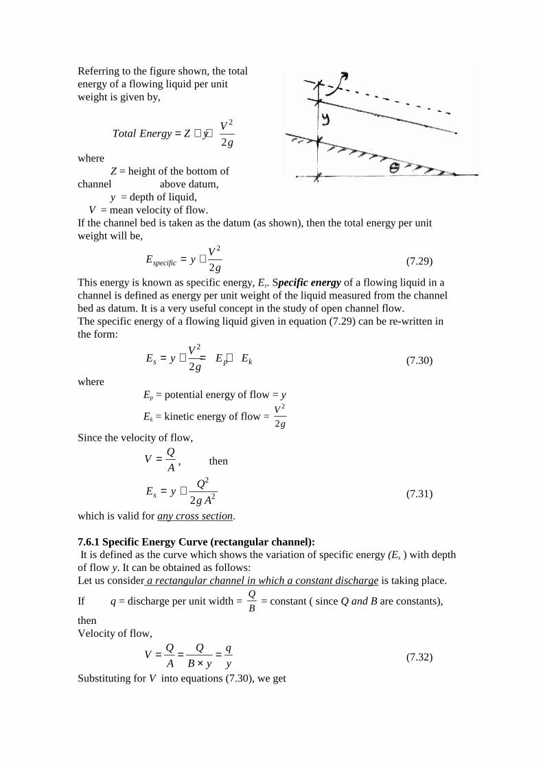
Referring to the figure shown, the total energy of a flowing liquid per unit weight is given by,

Total Energy Z yV

g= + +

2

2

where Z = height of the bottom of channel above datum, y = depth of liquid, V = mean velocity of flow. If the channel bed is taken as the datum (as shown), then the total energy per unit weight will be,

E yV

gspecific = +2

2 (7.29)

This energy is known as specific energy, Es. Specific energy of a flowing liquid in a channel is defined as energy per unit weight of the liquid measured from the channel bed as datum. It is a very useful concept in the study of open channel flow. The specific energy of a flowing liquid given in equation (7.29) can be re-written in the form:

E yV

gE Es p k= + = +

2

2 (7.30)

where Ep = potential energy of flow = y

Ek = kinetic energy of flow = V

g

2

2

Since the velocity of flow,

VQ

A= , then

E yQ

g As = +

2

22 (7.31)

which is valid for any cross section. 7.6.1 Specific Energy Curve (rectangular channel): It is defined as the curve which shows the variation of specific energy (Es ) with depth of flow y. It can be obtained as follows: Let us consider a rectangular channel in which a constant discharge is taking place.

If q = discharge per unit width = Q

B = constant ( since Q and B are constants),

then Velocity of flow,

VQ

A

Q

B y

q

y= =

×= (7.32)

Substituting for V into equations (7.30), we get

E yq

g yE Es p k= + = +

2

22 (7.33)

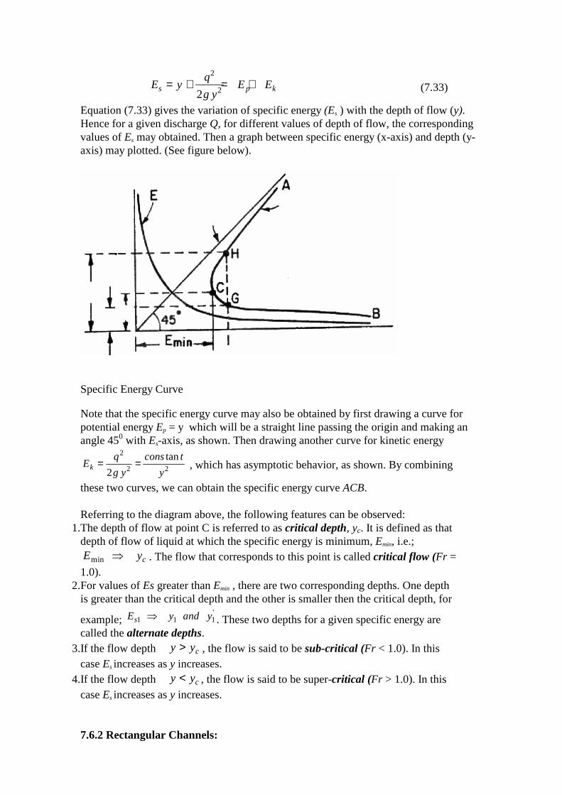
Equation (7.33) gives the variation of specific energy (Es ) with the depth of flow (y). Hence for a given discharge Q, for different values of depth of flow, the corresponding values of Es may obtained. Then a graph between specific energy (x-axis) and depth (y-axis) may plotted. (See figure below).

Specific Energy Curve Note that the specific energy curve may also be obtained by first drawing a curve for potential energy Ep = y which will be a straight line passing the origin and making an angle 450 with Es-axis, as shown. Then drawing another curve for kinetic energy

Eq

g y

cons t

yk = =

2

2 22

tan , which has asymptotic behavior, as shown. By combining

these two curves, we can obtain the specific energy curve ACB. Referring to the diagram above, the following features can be observed:

1.The depth of flow at point C is referred to as critical depth, yc. It is defined as that depth of flow of liquid at which the specific energy is minimum, Emin, i.e.; E ycmin ⇒ . The flow that corresponds to this point is called critical flow (Fr = 1.0).

2.For values of Es greater than Emin , there are two corresponding depths. One depth is greater than the critical depth and the other is smaller then the critical depth, for

example; E y and ys1 1 1⇒ '. These two depths for a given specific energy are

called the alternate depths. 3.If the flow depth y yc> , the flow is said to be sub-critical (Fr < 1.0). In this

case Es increases as y increases. 4.If the flow depth y yc< , the flow is said to be super-critical (Fr > 1.0). In this

case Es increases as y increases. 7.6.2 Rectangular Channels:

a) Critical depth, yc , is defined as that depth of flow of liquid at which the specific energy is minimum, Emin, see figure above. The mathematical expression for critical depth is obtained by differentiating equation (7.33) with respect to y and equationg the

result to zero, i.e.; dE

dy= 0

d

dyy

q

g y

q

g y( ) ( )+ = + − =

2

2

2

321

2

20 , or

1 02

33

2

− = ⇒ =q

g yy

q

g , or

yq

g=

213

and since for E = Emin , y = yc , therefore for rectangular channel

yq

gc =

213

(7.34)

b) Critical velocity, Vc , is the velocity of flow at critical depth. Cubing both sides of equation (7.34), we can write

yq

gc3

2

= (7.35)

and from equation (7.32) we have Vq

ycc

= , or

yV y

gcc c32 2

= and therefore

V g yc c= × (7.36)

c) Critical, Sub-critical, and Super-critical Flows: Critical flow is defined as the flow at which the specific energy is minimum or the flow that corresponds to critical depth. Refer to point C in above figure, E ycmin ⇒ . Equation (7.36) gives the relation for critical velocity in terms of critical depth as

V g yc c= × or

V

g yc

c×= 1 (7.37)

and recalling that Froude number is FrV

g D= , therefore for critical flow Fr = 1.0 .

If the depth flow y yc> , the flow is said to be sub-critical. In this case Es increases as y increases. For this type of flow, Fr < 1.0 . If the depth flow y yc< , the flow is said to be super-critical. In this case Es increases as y decreases. For this type of flow, Fr > 1.0 .

d) Minimum Specific Energy in terms of critical depth. At (Emin , yc ) , equation (7.33) can be written as

E yq

g yc

cmin = +

2

22, using equation (7.35), we can write

E yy

cc

min = +2

, and hence

Eyc

min =3

2 (7.38)

or yE

c =2

3min

(7.39)

7.6.3 Non-rectangular Channels: a) Critical depth, yc. An expression for the critical depth of non-rectangular channels can be obtained by differentiating equation (7.31) with respect to y and equating the result to zero, i.e.;

dE

dys = 0

d

dyy

Q

g A

Q

g A

dA

dy( ) ( )+ = − =

2

2

2

321

2

20 , (constant discharge is assumed)

or 1 02

3− =Q

g A

dA

dy( )

the term dA/dy represents the rate of increase of area with respect to y. A little reflection will show that it is equal to the top width T. Therefore

1 02

3− =Q T

g A

or Q

g

A

T

2 3

= (7.40)

This condition must be satisfied for the flow to occur at the critical depth. Recalling that hydraulic depth be definition is

DA

Th = so equation (7.34) can be written as

Q

gA Dh

22= (7.41)

Above equation may also be written in terms of velocity,

V

g

Dh2

2 2= (7.42)

this equation shows that the velocity head is equal to one-half the hydraulic depth for critical flow.

b) Constant specific energy. So far, the specific energy was varied and the discharge was assumed to be constant. Let us now consider the case in which the specific energy is kept constant and the discharge Q is varied. From equation (7.31) we may write

E yQ

g As − =

2

22 or

Q A g E ys= −2 ( ) , squaring both sides we get

Q A g E y gA E gA ys s2 2 2 22 2 2= − = −( ) ( )

For a given specific energy, the discharge will maximum if dQ

dy= 0 , differentiating

above equation yields

QdQ

dyg E A

dA

dyg y A

dA

dyAs= − +

2 2 2 2 2( ) ( )

using the fact that dA/dy = T and satisfy the above condition, we write

2 2 2 2 2 02g E AT g yAT gAs ( ) ( )− − = , or

4 4 2 0E T yT As − − = , or

2T E y As( )− = , or

E yA

Ts = +2 (7.43)

but E yQ

g As = +

2

22

therefore,

yQ

g Ay

A

T+ = +

2

22 2 , or

Q

g

A

T

2 3

= (7.40)

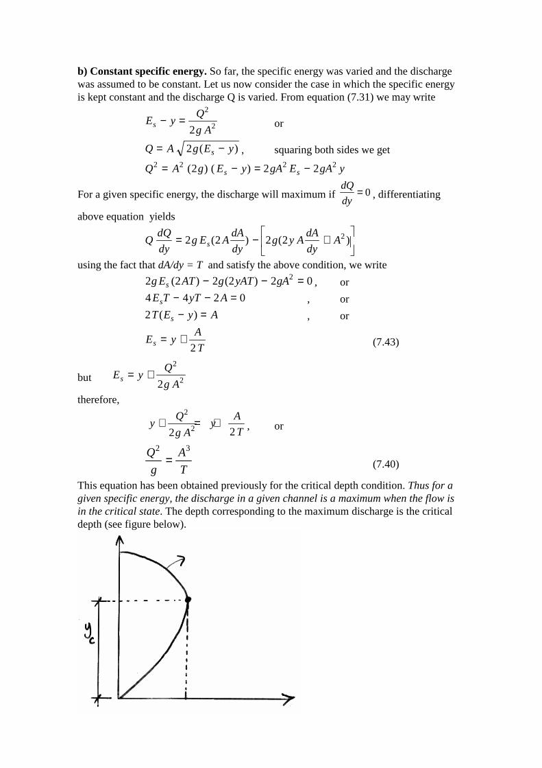
This equation has been obtained previously for the critical depth condition. Thus for a given specific energy, the discharge in a given channel is a maximum when the flow is in the critical state. The depth corresponding to the maximum discharge is the critical depth (see figure below).

c) Critical flow. In article 7.6.2, expressions for the critical depth in rectangular channels were obtained. Similar equations can be derived for non-rectangular channels. Equation (7.40) is the general equation for critical flow,

Q

g

A

T

2 3

= or Q

g A

A

T

2

2=

and form equation (7.31) we have

E yQ

g As = +

2

22 , therefore

E yA

Ts = +2

As this equation represents the critical state, it can be written as

E yA

Tc c= +1

2( )

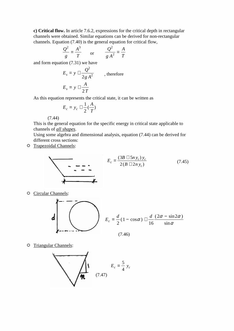
(7.44) This is the general equation for the specific energy in critical state applicable to channels of all shapes. Using some algebra and dimensional analysis, equation (7.44) can be derived for different cross sections:

� Trapezoidal Channels:

EB n y y

B n ycc c

c

=+

+( )

( )

3 5

2 2 (7.45)

� Circular Channels:

Ed d

c = − +−

21

16

2 2( cos )

( sin )

sinα α α

α

(7.46)

� Triangular Channels:

E yc c=5

4

(7.47)

In the above formulas, one must find yc first (except for circular channels). Condition given by equation (7.40) can be used to accomplish this. One may have to use trial and error scheme to find yc, specially in trapezoidal channels. 7.7 Non-uniform Flow in Open Channels:

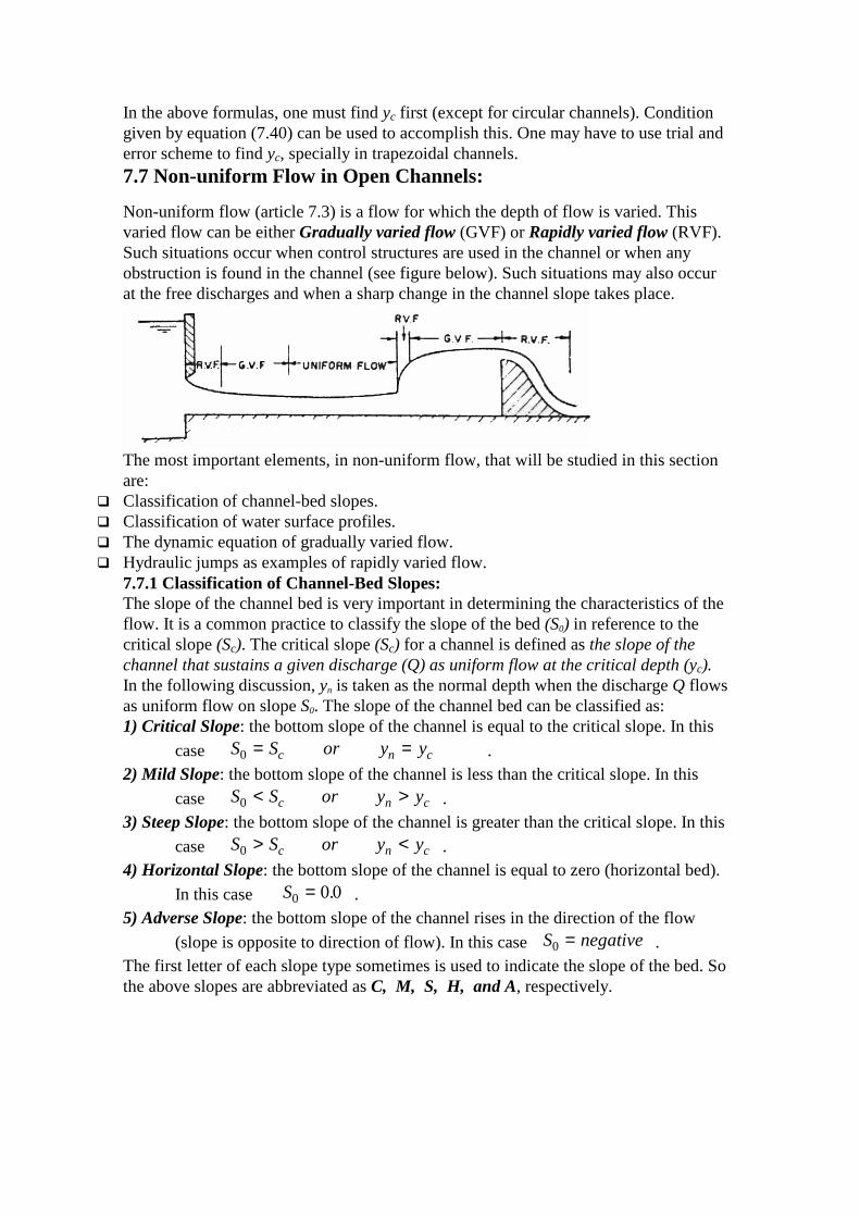
Non-uniform flow (article 7.3) is a flow for which the depth of flow is varied. This varied flow can be either Gradually varied flow (GVF) or Rapidly varied flow (RVF). Such situations occur when control structures are used in the channel or when any obstruction is found in the channel (see figure below). Such situations may also occur at the free discharges and when a sharp change in the channel slope takes place.

The most important elements, in non-uniform flow, that will be studied in this section are:

� Classification of channel-bed slopes. � Classification of water surface profiles. � The dynamic equation of gradually varied flow. � Hydraulic jumps as examples of rapidly varied flow.

7.7.1 Classification of Channel-Bed Slopes: The slope of the channel bed is very important in determining the characteristics of the flow. It is a common practice to classify the slope of the bed (S0) in reference to the critical slope (Sc). The critical slope (Sc) for a channel is defined as the slope of the channel that sustains a given discharge (Q) as uniform flow at the critical depth (yc). In the following discussion, yn is taken as the normal depth when the discharge Q flows as uniform flow on slope S0. The slope of the channel bed can be classified as: 1) Critical Slope: the bottom slope of the channel is equal to the critical slope. In this

case S S or y yc n c0 = = . 2) Mild Slope: the bottom slope of the channel is less than the critical slope. In this

case S S or y yc n c0 < > . 3) Steep Slope: the bottom slope of the channel is greater than the critical slope. In this

case S S or y yc n c0 > < . 4) Horizontal Slope: the bottom slope of the channel is equal to zero (horizontal bed).

In this case S0 0 0= . . 5) Adverse Slope: the bottom slope of the channel rises in the direction of the flow

(slope is opposite to direction of flow). In this case S negative0 = . The first letter of each slope type sometimes is used to indicate the slope of the bed. So the above slopes are abbreviated as C, M, S, H, and A, respectively.

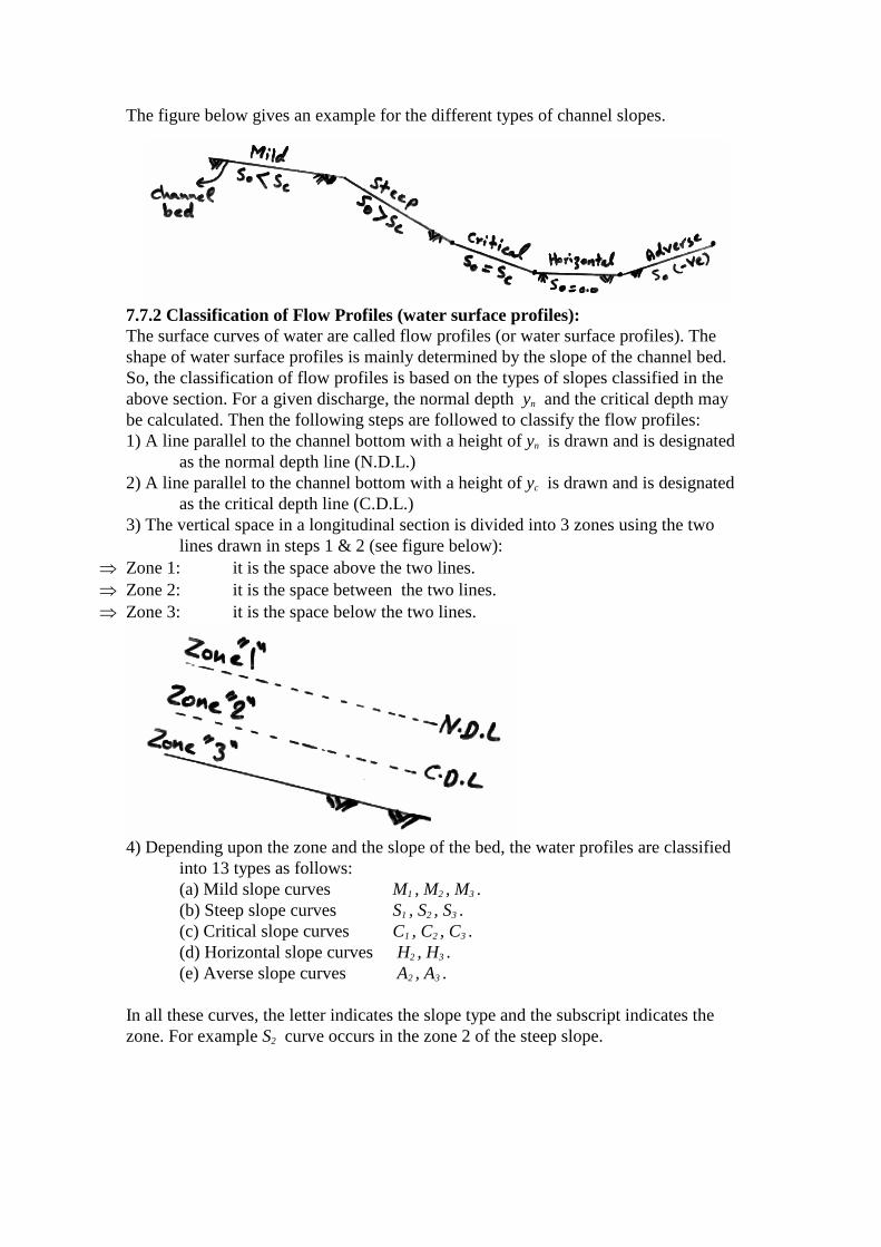
The figure below gives an example for the different types of channel slopes.

7.7.2 Classification of Flow Profiles (water surface profiles): The surface curves of water are called flow profiles (or water surface profiles). The shape of water surface profiles is mainly determined by the slope of the channel bed. So, the classification of flow profiles is based on the types of slopes classified in the above section. For a given discharge, the normal depth yn and the critical depth may be calculated. Then the following steps are followed to classify the flow profiles: 1) A line parallel to the channel bottom with a height of yn is drawn and is designated as the normal depth line (N.D.L.) 2) A line parallel to the channel bottom with a height of yc is drawn and is designated as the critical depth line (C.D.L.) 3) The vertical space in a longitudinal section is divided into 3 zones using the two lines drawn in steps 1 & 2 (see figure below):

⇒ Zone 1: it is the space above the two lines. ⇒ Zone 2: it is the space between the two lines. ⇒ Zone 3: it is the space below the two lines.

4) Depending upon the zone and the slope of the bed, the water profiles are classified into 13 types as follows: (a) Mild slope curves M1 , M2 , M3 . (b) Steep slope curves S1 , S2 , S3 . (c) Critical slope curves C1 , C2 , C3 . (d) Horizontal slope curves H2 , H3 . (e) Averse slope curves A2 , A3 . In all these curves, the letter indicates the slope type and the subscript indicates the zone. For example S2 curve occurs in the zone 2 of the steep slope.

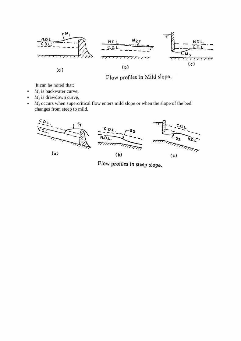
It can be noted that:

• M1 is backwater curve, • M2 is drawdown curve, • M3 occurs when supercritical flow enters mild slope or when the slope of the bed

changes from steep to mild.

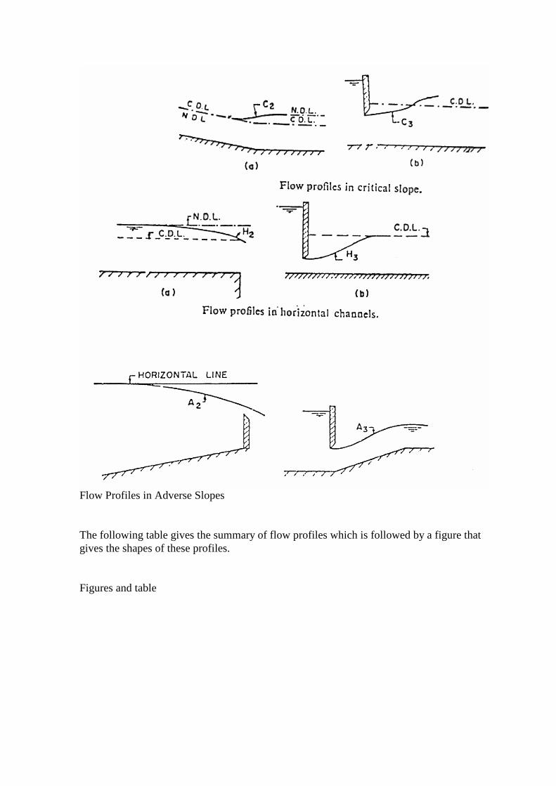
Flow Profiles in Adverse Slopes The following table gives the summary of flow profiles which is followed by a figure that gives the shapes of these profiles. Figures and table

7.7.3 Dynamic Equation of Gradually Varied Flow: The dynamic equation of gradually varied flow is an expression giving the relationship between the water surface slope and other characteristics of flow. The following assumptions are made in the derivation of the equation:

(1) The flow is steady: depth and other hydraulic characteristics at a particular section do not change with time.

(2) The streamlines are practically parallel: which is true when the variation in depth along the direction of flow is very gradual. Thus the hydrostatic distribution of pressure is assumed over the section.

(3) The loss of head at any section, due to friction, in gradually varied flow is equal to that in the corresponding uniform flow with the same depth and flow characteristics. According to this assumption, the uniform flow formulas, such as Manning’s formula, may be used to calculate the slope of the energy line (Sf) in gradually varied flow as well.

(4) The slope of the channel is small: for small slopes, the depth of flow is approximately equal to the depth of flow section, i.e.; y D= .

(5) The channel is prismatic, i.e.; it has constant shape, size, slope and alignment. (6) The velocity distribution across the section is fixed. (7) The roughness coefficient (Manning’s coefficient) is constant in the reach. Also, it

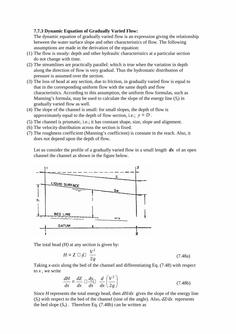
does not depend upon the depth of flow. Let us consider the profile of a gradually varied flow in a small length dx of an open channel the channel as shown in the figure below.

The total head (H) at any section is given by:

H Z yV

g= + +

2

2 (7.48a)

Taking x-axis along the bed of the channel and differentiating Eq. (7.48) with respect to x , we write

dH

dx

dZ

dx

dy

dx

d

dx

V

g= + +

2

2 (7.48b)

Since H represents the total energy head, then dH/dx gives the slope of the energy line (Sf) with respect to the bed of the channel (sine of the angle). Also, dZ/dx represents the bed slope (S0) . Therefore Eq. (7.48b) can be written as

− = − + +

S S

dy

dx

d

dx

V

gf 0

2

2

Multiplying the velocity term by dy/dy and transposing, we get

dy

dx

dy

dy

d

dx

V

gS Sf+

= −

2

02

or dy

dx

d

dy

V

gS Sf1

2

2

0+

= −

dy

dx

S S

d

dy

V

g

f=

−

+

0

2

12

(7.49)

Equation (7.49) is known as the dynamic equation of gradually varied flow. It gives the slope of the water surface with respect to the bottom of the channel. In other words, it gives the variation of depth (y) with respect to the distance along the bottom of the channel (x). The dynamic equation (7.49) can be expressed in terms of the discharge Q ,

dy

dx

S S

Q T

g A

f=−

−

02

31

(7.50)

The dynamic equation (7.49) also can be expressed in terms of the specific energy E ,

dy

dx

dE dx

Q T

g A

=−

/

12

3

(7.50) Depending upon the type of flow, dy/dx may take the values:

(a) dy

dx= 0 : this indicates that the slope of the water surface is equal to the bottom

slope. This indicates that the slope of the water surface is equal to the bottom slope. In other words, the water surface is parallel to the channel bed. The flow is uniform.

(b) dy

dxpositive= : this indicates that the slope of the water surface is less than the

bottom slope (S0) . In this case , the water surface rises in the direction of flow. The profile so obtained is called the backwater curve.

(c) dy

dxnegative= : this indicates that the slope of the water surface is greater than the

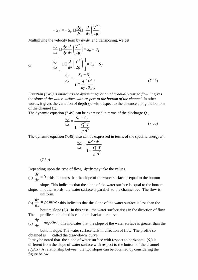
bottom slope. The water surface falls in direction of flow. The profile so obtained is called the draw-down curve. It may be noted that the slope of water surface with respect to horizontal (Sw) is different from the slope of water surface with respect to the bottom of the channel (dy/dx). A relationship between the two slopes can be obtained by considering the figure below.

Consider a small length dx of the open channel. The line ab shows the free surface, the line ad is drawn parallel to the bottom at a slope of S0 with the horizontal. The line ac is horizontal. The water surface slope (Sw) is given by

Sbc

ab

cd bd

abw = = =−

sinφ (7.50a)

Let θ be the angle which the bottom makes with the horizontal. Thus

Scd

ad

cd

ab0 = = ≈sinθ (7.50b)

The slope of the water surface with respect to the channel bottom is given by

dy

dx

bd

ad

bd

ab= ≈ (7.50c)

Substitute Eqns. (7.50b) and (7.50c) into Eqn. (7.50a),

S Sdy

dxw = −0 (7.51a)

This equation can be used to calculate the water surface slope with respect to horizontal. Also, it can be written as

dy

dxS Sw= −0 (7.51b)

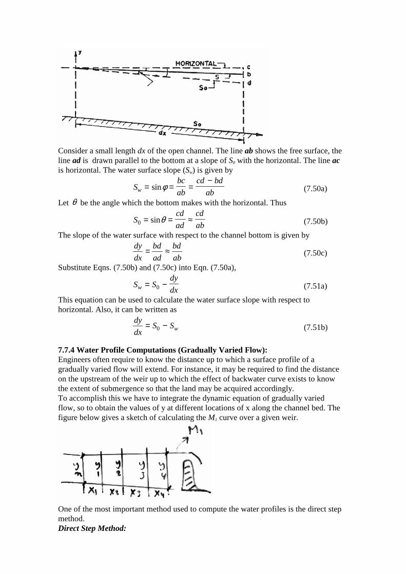
7.7.4 Water Profile Computations (Gradually Varied Flow): Engineers often require to know the distance up to which a surface profile of a gradually varied flow will extend. For instance, it may be required to find the distance on the upstream of the weir up to which the effect of backwater curve exists to know the extent of submergence so that the land may be acquired accordingly. To accomplish this we have to integrate the dynamic equation of gradually varied flow, so to obtain the values of y at different locations of x along the channel bed. The figure below gives a sketch of calculating the M1 curve over a given weir.

One of the most important method used to compute the water profiles is the direct step method. Direct Step Method:

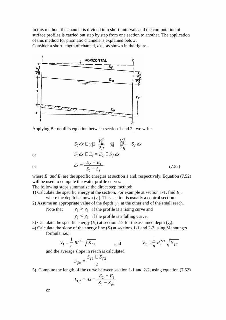
In this method, the channel is divided into short intervals and the computation of surface profiles is carried out step by step from one section to another. The application of this method for prismatic channels is explained below. Consider a short length of channel, dx , as shown in the figure.

Applying Bernoulli’s equation between section 1 and 2 , we write

S dx yV

gy

V

gS dxf0 1

12

222

2 2+ + = + +

or S dx E E S dxf0 1 2+ = +

or dxE E

S Sf

=−−

2 1

0 (7.52)

where E1 and E2 are the specific energies at section 1 and, respectively. Equation (7.52) will be used to compute the water profile curves. The following steps summarize the direct step method: 1) Calculate the specific energy at the section. For example at section 1-1, find E1, where the depth is known (y1). This section is usually a control section. 2) Assume an appropriate value of the depth y2 at the other end of the small reach. Note that y y2 1> if the profile is a rising curve and

y y2 1< if the profile is a falling curve. 3) Calculate the specific energy (E2) at section 2-2 for the assumed depth (y2). 4) Calculate the slope of the energy line (Sf) at sections 1-1 and 2-2 using Mannung’s formula, i.e.;

Vn

R Sf1 12 3

1

1= /

and Vn

R Sf2 22 3

2

1= /

and the average slope in reach is calculated

SS S

fmf f

=+1 2

2

5) Compute the length of the curve between section 1-1 and 2-2, using equation (7.52)

L dxE E

S Sfm1

2 1

0,2 = =

−−

or

LE E

SS Sf f

1 22 1

01 2

2

, =−

−+

(7.53)

6) Now, we know the depth at section 2-2, we assume the depth at the next section, say 3-3. Then repeat the procedure to find the length L2,3. 7) Repeating the procedure, the total length of the curve may be obtained. Thus L L L Ln n= + + + −1 2 2 3 1, , ,.......

where (n-1) is the number of intervals into which the channel is divided. It may be noted that in sub-critical flow the computation is carried from downstream to upstream, whereas in supercritical flow from upstream to downstream. See Next Example. 7.7.5 Hydraulic Jump:

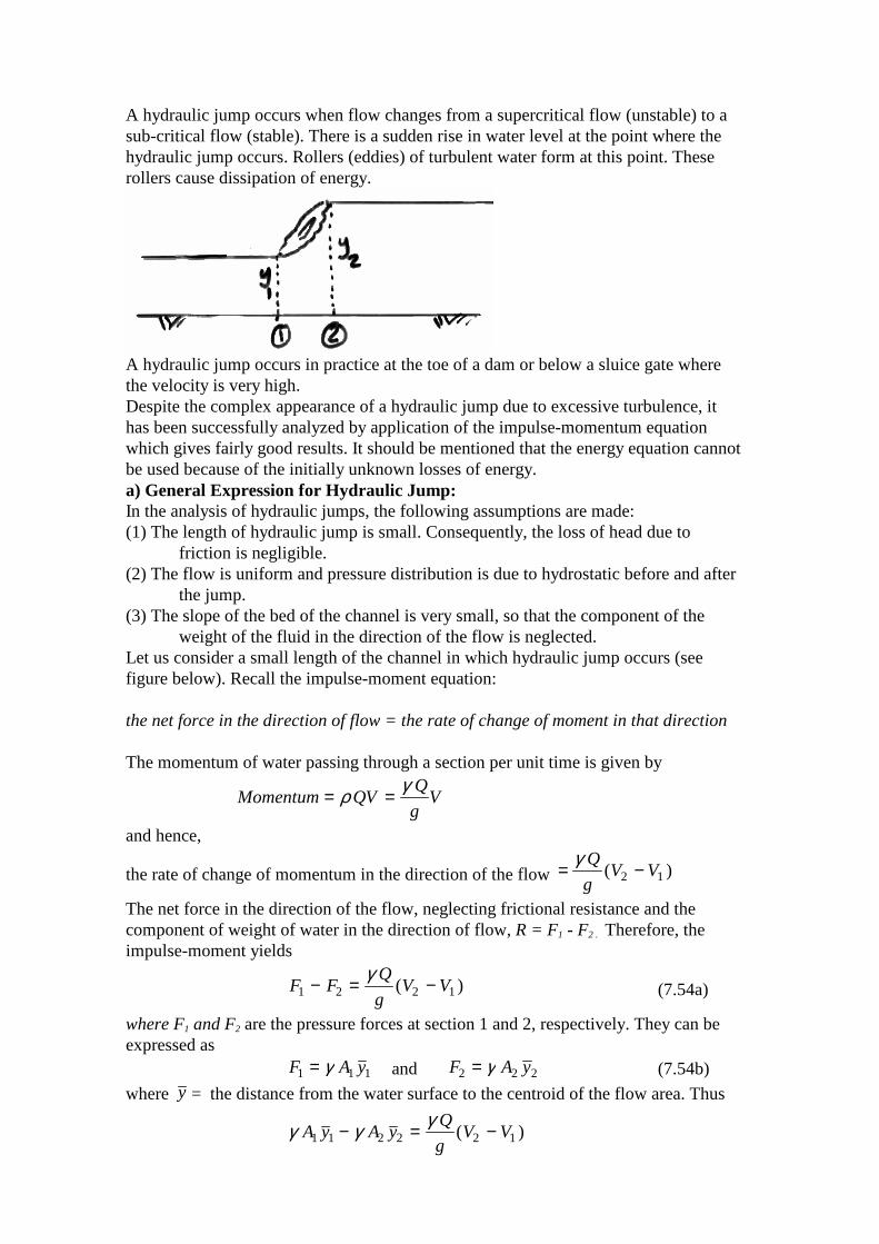
A hydraulic jump occurs when flow changes from a supercritical flow (unstable) to a sub-critical flow (stable). There is a sudden rise in water level at the point where the hydraulic jump occurs. Rollers (eddies) of turbulent water form at this point. These rollers cause dissipation of energy.

A hydraulic jump occurs in practice at the toe of a dam or below a sluice gate where the velocity is very high. Despite the complex appearance of a hydraulic jump due to excessive turbulence, it has been successfully analyzed by application of the impulse-momentum equation which gives fairly good results. It should be mentioned that the energy equation cannot be used because of the initially unknown losses of energy. a) General Expression for Hydraulic Jump: In the analysis of hydraulic jumps, the following assumptions are made: (1) The length of hydraulic jump is small. Consequently, the loss of head due to friction is negligible. (2) The flow is uniform and pressure distribution is due to hydrostatic before and after the jump. (3) The slope of the bed of the channel is very small, so that the component of the weight of the fluid in the direction of the flow is neglected. Let us consider a small length of the channel in which hydraulic jump occurs (see figure below). Recall the impulse-moment equation: the net force in the direction of flow = the rate of change of moment in that direction The momentum of water passing through a section per unit time is given by

Momentum QVQ

gV= =ρ γ

and hence,

the rate of change of momentum in the direction of the flow = −γ Q

gV V( )2 1

The net force in the direction of the flow, neglecting frictional resistance and the component of weight of water in the direction of flow, R = F1 - F2 . Therefore, the impulse-moment yields

F FQ

gV V1 2 2 1− = −γ

( ) (7.54a)

where F1 and F2 are the pressure forces at section 1 and 2, respectively. They can be expressed as F A y1 1 1= γ and F A y2 2 2= γ (7.54b)

where y = the distance from the water surface to the centroid of the flow area. Thus

γ γ γA y A y

Q

gV V1 1 2 2 2 1− = −( )

or γ γγ

A y A yQ

g A A1 1 2 2

2

2 1

1 1− = −( )

or Q

gAA y

Q

gAA y

2

11 1

2

22 2+ = + (7.55)

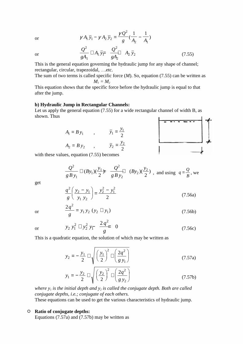
This is the general equation governing the hydraulic jump for any shape of channel; rectangular, circular, trapezoidal, ….etc. The sum of two terms is called specific force (M). So, equation (7.55) can be written as M1 = M2 This equation shows that the specific force before the hydraulic jump is equal to that after the jump. b) Hydraulic Jump in Rectangular Channels: Let us apply the general equation (7.55) for a wide rectangular channel of width B, as shown. Thus

A B y1 1= , yy

11

2=

A B y2 2= , yy

22

2=

with these values, equation (7.55) becomes

Q

g B yBy

y Q

g B yBy

y2

11

12

22

2

2 2+ = +( )( ) ( )( ) , and using q

Q

B= , we

get

q

g

y y

y y

y y22 1

1 2

22

12

2

−

=

− (7.56a)

or 2 2

1 2 2 1q

gy y y y= +( ) (7.56b)

or y y y yq

g2 12

22

1

220+ − = (7.56c)

This is a quadratic equation, the solution of which may be written as

yy y q

g y21 1

2 2

12 2

2= − +

+

(7.57a)

yy y q

g y12 2

2 2

22 2

2= − +

+

(7.57b)

where y1 is the initial depth and y2 is called the conjugate depth. Both are called conjugate depths, i.e.; conjugate of each others. These equations can be used to get the various characteristics of hydraulic jump.

� Ratio of conjugate depths: Equations (7.57a) and (7.57b) may be written as

y

y

q

g y2

1

2

13

1

21 1

8= − + +

(7.58a)

y

y

q

g y1

2

2

23

1

21 1

8= − + +

(7.58a)

But for rectangular channels, we have

yq

gc3

2

= (7.35)

therefore,

y

y

y

yc2

1 1

31

21 1 8= − + +

(7.59a)

y

y

y

yc1

2 2

31

21 1 8= − + +

(7.59b)

These equations can also be written in terms of Froude’s number as

y

yF2

1121

21 1 8= − + +

(7.60a)

y

yF1

2221

21 1 8= − + +

(7.60a)

where FV

g y1

1

1

= and FV

g y2

2

2

=

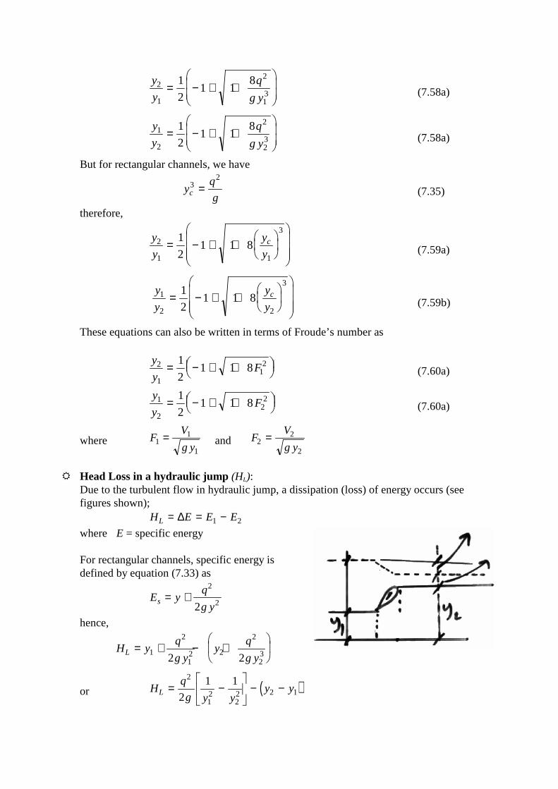
� Head Loss in a hydraulic jump (HL): Due to the turbulent flow in hydraulic jump, a dissipation (loss) of energy occurs (see figures shown); H E E EL = = −∆ 1 2

where E = specific energy For rectangular channels, specific energy is defined by equation (7.33) as

E yq

g ys = +

2

22

hence,

H yq

g yy

q

g yL = + − +

1

2

12 2

2

232 2

or ( )Hq

g y yy yL = −

− −

2

12

22 2 12

1 1

or ( )Hq

g

y y

y yy yL = −

− −

222

12

12

23 2 12

using equation (7.56b), we get

( )Hy y y y y y

y yy yL = + − − −1 2 1 2 2

212

12

22 2 1

4

( ) ( )

after simplifying, we obtain

Hy y

y yL =−( )2 1

3

1 24 (7.61)

� Height of hydraulic jump (hj):

The difference of depths before and after the jump is known as the height of the jump,

h y yj = −2 1 (7.62)

� Length of hydraulic jump (Lj):

The distance between the front face of the jump to a point on the downstream where the rollers (eddies) terminate and the flow becomes uniform is known as the length of the hydraulic jump. The length of the jump varies from 5 to 7 times its height. An average value is usually taken:

L hj j≅ 6 (7.63)

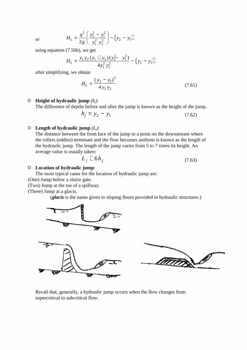
� Location of hydraulic jump: The most typical cases for the location of hydraulic jump are:

(One) Jump below a sluice gate. (Two) Jump at the toe of a spillway.

(Three) Jump at a glacis.

(glacis is the name given to sloping floors provided in hydraulic structures.)

Recall that, generally, a hydraulic jump occurs when the flow changes from supercritical to subcritical flow.