Chapter 7The Schroedinger Equation in One Dimension

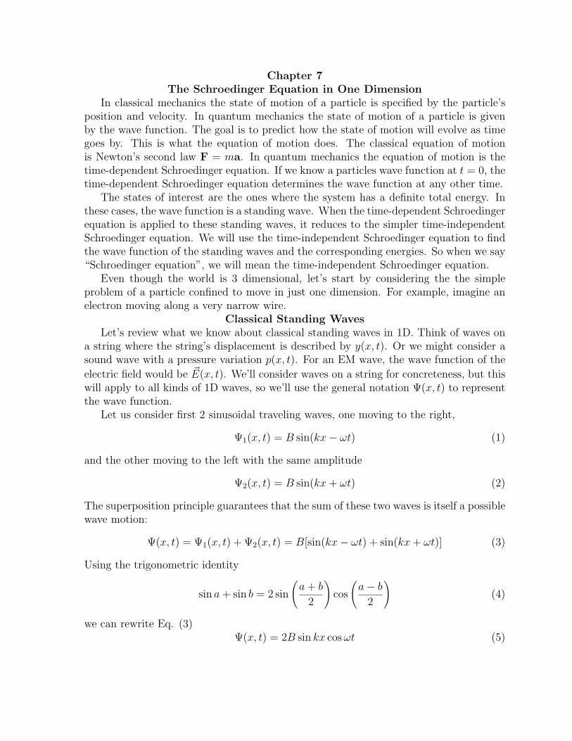
In classical mechanics the state of motion of a particle is specified by the particle’sposition and velocity. In quantum mechanics the state of motion of a particle is givenby the wave function. The goal is to predict how the state of motion will evolve as timegoes by. This is what the equation of motion does. The classical equation of motionis Newton’s second law F = ma. In quantum mechanics the equation of motion is thetime-dependent Schroedinger equation. If we know a particles wave function at t = 0, thetime-dependent Schroedinger equation determines the wave function at any other time.

The states of interest are the ones where the system has a definite total energy. Inthese cases, the wave function is a standing wave. When the time-dependent Schroedingerequation is applied to these standing waves, it reduces to the simpler time-independentSchroedinger equation. We will use the time-independent Schroedinger equation to findthe wave function of the standing waves and the corresponding energies. So when we say“Schroedinger equation”, we will mean the time-independent Schroedinger equation.

Even though the world is 3 dimensional, let’s start by considering the the simpleproblem of a particle confined to move in just one dimension. For example, imagine anelectron moving along a very narrow wire.

Classical Standing WavesLet’s review what we know about classical standing waves in 1D. Think of waves on

a string where the string’s displacement is described by y(x, t). Or we might consider asound wave with a pressure variation p(x, t). For an EM wave, the wave function of the

electric field would be ~E(x, t). We’ll consider waves on a string for concreteness, but thiswill apply to all kinds of 1D waves, so we’ll use the general notation Ψ(x, t) to representthe wave function.

Let us consider first 2 sinusoidal traveling waves, one moving to the right,

Ψ1(x, t) = B sin(kx− ωt) (1)

and the other moving to the left with the same amplitude

Ψ2(x, t) = B sin(kx+ ωt) (2)

The superposition principle guarantees that the sum of these two waves is itself a possiblewave motion:

Ψ(x, t) = Ψ1(x, t) + Ψ2(x, t) = B[sin(kx− ωt) + sin(kx+ ωt)] (3)

Using the trigonometric identity

sin a+ sin b = 2 sin

(

a+ b

2

)

cos

(

a− b

2

)

(4)

we can rewrite Eq. (3)Ψ(x, t) = 2B sin kx cosωt (5)

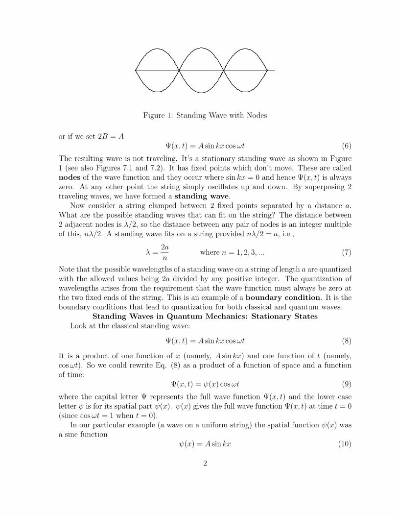
Figure 1: Standing Wave with Nodes

or if we set 2B = AΨ(x, t) = A sin kx cosωt (6)

The resulting wave is not traveling. It’s a stationary standing wave as shown in Figure1 (see also Figures 7.1 and 7.2). It has fixed points which don’t move. These are callednodes of the wave function and they occur where sin kx = 0 and hence Ψ(x, t) is alwayszero. At any other point the string simply oscillates up and down. By superposing 2traveling waves, we have formed a standing wave.

Now consider a string clamped between 2 fixed points separated by a distance a.What are the possible standing waves that can fit on the string? The distance between2 adjacent nodes is λ/2, so the distance between any pair of nodes is an integer multipleof this, nλ/2. A standing wave fits on a string provided nλ/2 = a, i.e.,

λ =2a

nwhere n = 1, 2, 3, ... (7)

Note that the possible wavelengths of a standing wave on a string of length a are quantizedwith the allowed values being 2a divided by any positive integer. The quantization ofwavelengths arises from the requirement that the wave function must always be zero atthe two fixed ends of the string. This is an example of a boundary condition. It is theboundary conditions that lead to quantization for both classical and quantum waves.

Standing Waves in Quantum Mechanics: Stationary StatesLook at the classical standing wave:

Ψ(x, t) = A sin kx cosωt (8)

It is a product of one function of x (namely, A sin kx) and one function of t (namely,cosωt). So we could rewrite Eq. (8) as a product of a function of space and a functionof time:

Ψ(x, t) = ψ(x) cosωt (9)

where the capital letter Ψ represents the full wave function Ψ(x, t) and the lower caseletter ψ is for its spatial part ψ(x). ψ(x) gives the full wave function Ψ(x, t) at time t = 0(since cosωt = 1 when t = 0).

In our particular example (a wave on a uniform string) the spatial function ψ(x) wasa sine function

ψ(x) = A sin kx (10)

2

i

sin

cos

y (imaginary part)

x (real part)

1θ

θ

θ

e = cos + i sinθ θθ

Figure 2: Complex number in the complex plane represented with polar angle θ.

but in more complicated problems, ψ(x) can be a more complicated function of x. Evenin these more complicated problems, the time dependence is still sinusoidal. It could bea sine or a cosine; the difference being just the choice in the origin of the time. Thegeneral sinusoidal standing wave is a combination of both:

Ψ(x, t) = ψ(x)(a cosωt+ b sinωt) (11)

Different choices for the ratio of the coefficients a and b correspond to different choicesof the origin of time. For a classical wave, the function Ψ(x, t) is a real number, and thecoefficients a and b in (11) are always real. In quantum mechanics, on the other hand,the wave function can be a complex number, and for quantum standing waves it usuallyis complex. Specifically, the time-dependent part of the wave function (11) is given by

cosωt− i sinωt (12)

That is, the standing waves of a quantum particle have the form

Ψ(x, t) = ψ(x)(cosωt− i sinωt) (13)

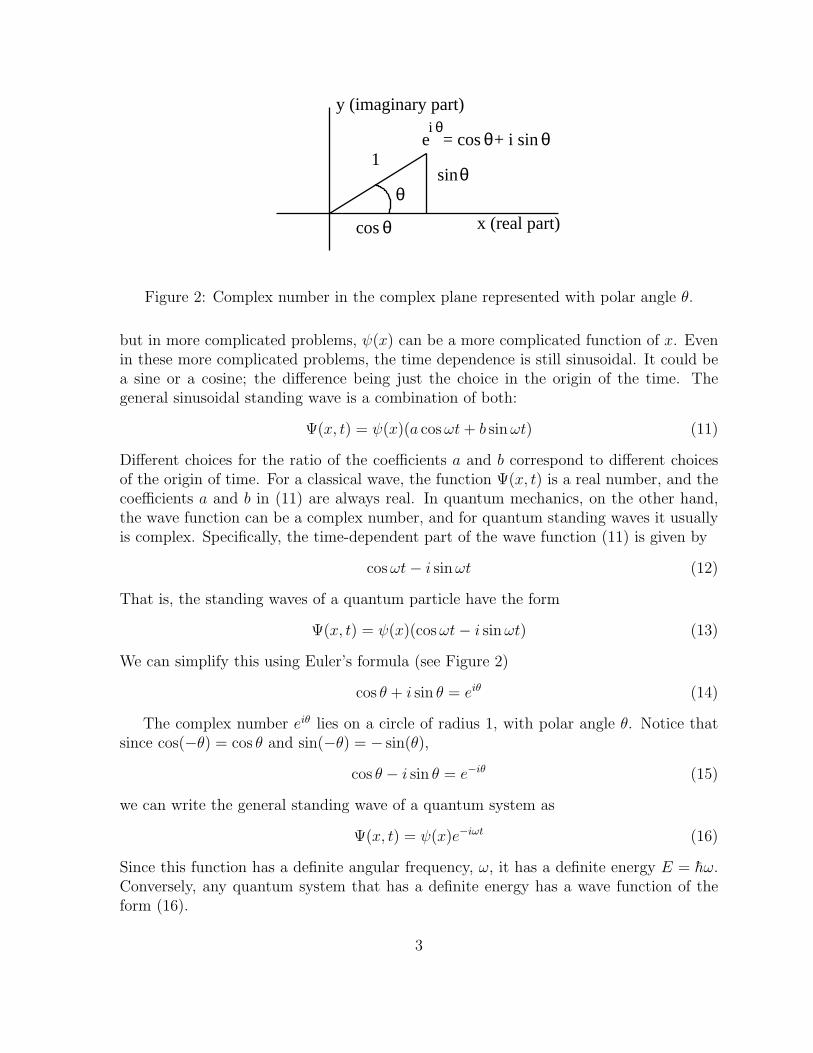
We can simplify this using Euler’s formula (see Figure 2)

cos θ + i sin θ = eiθ (14)

The complex number eiθ lies on a circle of radius 1, with polar angle θ. Notice thatsince cos(−θ) = cos θ and sin(−θ) = − sin(θ),

cos θ − i sin θ = e−iθ (15)

we can write the general standing wave of a quantum system as

Ψ(x, t) = ψ(x)e−iωt (16)

Since this function has a definite angular frequency, ω, it has a definite energy E = h̄ω.Conversely, any quantum system that has a definite energy has a wave function of theform (16).

3

The probability density associated with a quantum wave function Ψ(x, t) is the ab-solute value squared, |Ψ(x, t)|2.

|Ψ(x, t)|2 = |ψ(x)|2|e−iωt|2 = |ψ(x)|2 (17)

Thus, for a quantum standing wave, the probability density is independent of time. Fora quantum standing wave, the distribution of matter is time independent or stationary.This is why it’s called a stationary state. These are states of definite energy. Becausetheir charge distribution is static, atoms in stationary states do not radiate.

The interesting part of the wave function Ψ(x, t) is its spatial part ψ(x). We willsee that a large part of quantum mechanics is devoted to finding the possible spatialfunctions ψ(x) and their corresponding energies. Our principal tool in finding these willbe the time-independent Schroedinger equation.

The Particle in a Rigid BoxConsider a particle that is confined to some finite interval on the x axis, and moves

freely inside that interval. This is a one-dimensional rigid box, and is often called theinfinite square well. An example would be an electron inside a length of very thinconducting wire. The electron would move freely back and forth inside the wire, butcould not escape from it.

Consider a quantum particle of mass m moving in a 1D rigid box of length a, with noforces acting on it inside the box between x = 0 and x = a. So the potential U = 0 insidethe box. Therefore, the particle’s total energy is just its kinetic energy. In quantummechanics, we write the kinetic energy as p2/2m, rather than 1

2mv2, because of the de

Broglie relation, λ = h/p. (This will make more sense later.) So we write the energy as

E = K =p2

2m(18)

States of definite energy are standing waves that have the form

Ψ(x, t) = ψ(x)e−iωt (19)

By analogy with waves on a string, one might guess that the spatial function would havethe form

ψ(x) = A sin kx+B cos kx (20)

for 0 ≤ x ≤ a.Since it is impossible for the particle to escape from the box, the wave function must

be zero outside; that is ψ(x) = 0 when x < 0 and when x > a. If we assume that ψ(x)is continuous, then it must also vanish at x = 0 and x = a:

ψ(0) = ψ(a) = 0 (21)

These boundary conditions are identical to those for a classical wave on a string clampedat x = 0 and x = a.

4

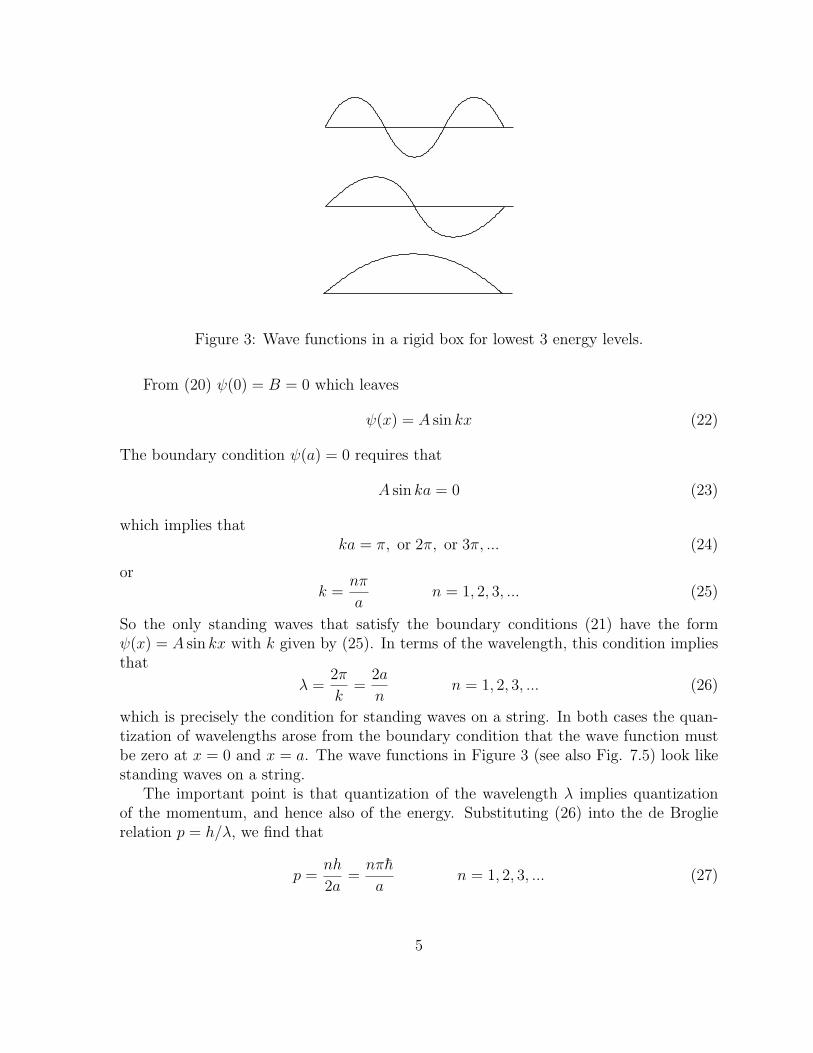
Figure 3: Wave functions in a rigid box for lowest 3 energy levels.

From (20) ψ(0) = B = 0 which leaves

ψ(x) = A sin kx (22)

The boundary condition ψ(a) = 0 requires that

A sin ka = 0 (23)

which implies thatka = π, or 2π, or 3π, ... (24)

ork =

nπ

an = 1, 2, 3, ... (25)

So the only standing waves that satisfy the boundary conditions (21) have the formψ(x) = A sin kx with k given by (25). In terms of the wavelength, this condition impliesthat

λ =2π

k=

2a

nn = 1, 2, 3, ... (26)

which is precisely the condition for standing waves on a string. In both cases the quan-tization of wavelengths arose from the boundary condition that the wave function mustbe zero at x = 0 and x = a. The wave functions in Figure 3 (see also Fig. 7.5) look likestanding waves on a string.

The important point is that quantization of the wavelength λ implies quantizationof the momentum, and hence also of the energy. Substituting (26) into the de Broglierelation p = h/λ, we find that

p =nh

2a=nπh̄

an = 1, 2, 3, ... (27)

5

Plugging this into E = p2/2m yields

En = n2 π2h̄2

2ma2n = 1, 2, 3, ... (28)

The ground state energy is obtained for n = 1:

E1 =π2h̄2

2ma2(29)

This is consistent with the lower bound derived from the Heisenberg uncertainty principlefor a particle confined in a region of length a:

E ≥ h̄2

2ma2(30)

The actual minimum energy (29) is larger than the lower bound (30) by a factor ofπ2 ≈ 10. In terms of the ground state energy E1, the energy of the nth level (28) is

En = n2E1 n = 1, 2, 3, ... (31)

Note that the energy levels are farther and farther apart as n increases and that En

increases without limit as n→ ∞. The number of nodes of the wave functions increasessteadily with energy; this is what one should expect since more nodes mean shorterwavelength (larger curvature of ψ) and hence larger momentum and kinetic energy. Youcan see this from

p =h

λ

E =p2

2m=

h2

2mλ2

The complete wave function Ψ(x, t) for any of our standing waves has the form

Ψ(x, t) = ψ(x)e−iωt = A sin(kx)e−iωt (32)

Using the identity

sin θ =eiθ − e−iθ

2i(33)

we can write

Ψ(x, t) =A

2i

(

ei(kx−ωt) − e−i(kx+ωt))

(34)

Thus, our quantum standing wave (just like the classical standing wave) can be expressedas the sum of two traveling waves, one moving to the right and one moving to the left.The right-moving wave represents a particle with momentum hk directed to the right,and the left-moving wave represents a particle with momentum hk but directed to the

6

left. So a particle in a stationary state has momentum with magnitude hk but is anequal superposition of momenta in either direction. This corresponds to the result thaton average a classical particle is equally likely to be moving in either direction as itbounces back and forth inside a rigid box.

The Time-Independent Schroedinger EquationOur discussion of the particle in a rigid box required some guessing as to the form of

the spatial wave function ψ(x). We want to take the guesswork out of finding ψ(x). Sowe need an equation to determine ψ(x). This is what the time-independent Schroedingerequation does. Like all basic laws of physics, the Schroedinger equation cannot be derived.However, we can try to motivate it.

Almost all laws of physics can be expressed as differential equations. For example,Newton’s second law:

md2x

dt2=∑

F (35)

Another example is the equation of motion for classical waves which is a differentialequation. We expect the equation that determines the possible standing waves of aquantum system to be a differential equation. Since we already know the form of thewave functions for a particle in a box, we can try to spot a simple differential equationthat they satisfy and that we can generalize to more complicated systems.

ψ(x) = A sin kx

dψ

dx= kA cos kx

d2ψ

dx2= −k2A sin kx

d2ψ

dx2= −k2ψ (36)

We can rewrite k2 in (36) in terms of the particle’s kinetic energy K. Using p = h̄k, wehave

K =p2

2m=h̄2k2

2m(37)

k2 =2mK

h̄2(38)

d2ψ

dx2= −2mK

h̄2ψ (39)

Since the kinetic energy K is the difference between the total energy E and the potentialenergy U(x), we can replace K in (39) by

K = E − U(x) (40)

to getd2ψ

dx2=

2m

h̄2[U(x)− E]ψ (41)

7

This differential equation is called the Schroedinger equation, or more precisely, thetime-independent Schroedinger equation, in honor of the Austrian physicist, ErwinSchroedinger, who first published it in 1926. There is no way to prove that this equationis correct. But its predictions agree with experiment. Schroedinger himself showed thatit correctly predicts the energy levels of the hydrogen atom. The Schroedinger equationis the basis of nonrelativistic quantum mechanics.

Here is the general procedure for using the equation. Given a system whose stationarystates and energies we want to know, we must first find the potential energy functionU(x). For example, a particle in a harmonic oscillator potential (a spring potential) haspotential energy

U(x) =1

2kx2 (42)

Another example is an electron in a hydrogen atom:

U(x) = −ke2

r(43)

In most cases, it turns out that for many values of the energy E, the Schroedinger equationhas no solutions, i.e., no acceptable solutions satisfying the particular conditions of theproblem. This leads to the quantization of the energy. As a result, only certain values ofthe energy are allowed and these are called eigenvalues. Associated with each eigenvalueis a stationary wave function called an eigenfunction.

An acceptable solution must satisfy certain conditions. First ψ(x) may have to satisfyboundary conditions, e.g., ψ(x) must vanish at the walls of a perfectly rigid box withinfinitely high walls (U = ∞). Another condition is that ψ(x) must always be continuous,and in most problems, its first derivative must also be continuous. An acceptable solutionof the Schroedinger equation must satisfy all the conditions appropriate to the problemat hand.

Note that quantum mechanics focuses primarily on potential energies, whereas New-tonian mechanics focuses on forces.

The Rigid Box AgainAs a first application of the Schroedinger equation, we use it to rederive the allowed

energies of a particle in a rigid box and check that we get the same answers as before.We start by identifying the potential energy function U(x). Inside the box the potentialenergy is zero, and outside the box it is infinite. Thus

U(x) =

{

0 for 0 ≤ x ≤ a∞ for x < 0 and x > a

(44)

This potential energy function is often described as an infinitely deep square well becausea graph of U(x) looks like a well with infinitely high sides and square corners (see Figure4).

Since U(x) = ∞ outside the box, the particle can never be found there, so ψ(x) mustbe zero outside the box, i.e., when x < 0 and when x > a. The continuity of ψ(x) requires

8

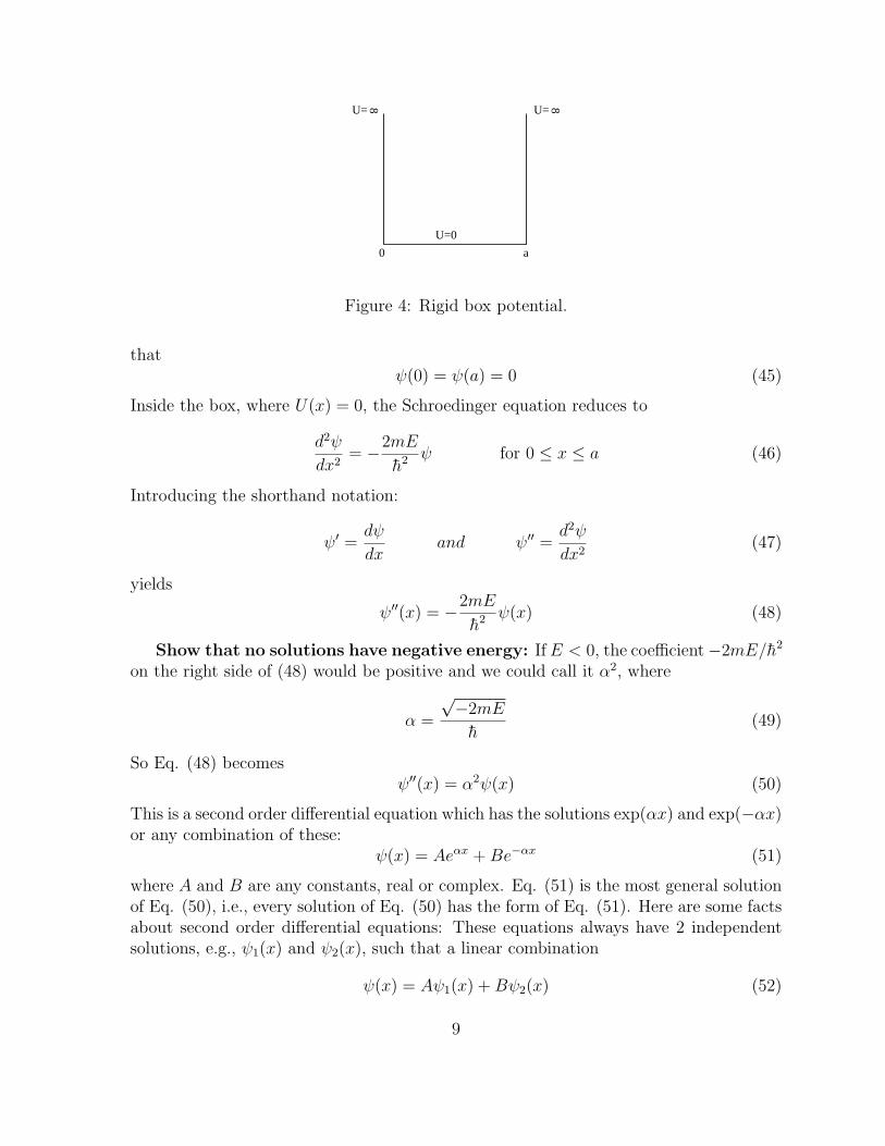
U=0

8U= 8

0 a

U=

Figure 4: Rigid box potential.

thatψ(0) = ψ(a) = 0 (45)

Inside the box, where U(x) = 0, the Schroedinger equation reduces to

d2ψ

dx2= −2mE

h̄2ψ for 0 ≤ x ≤ a (46)

Introducing the shorthand notation:

ψ′ =dψ

dxand ψ′′ =

d2ψ

dx2(47)

yields

ψ′′(x) = −2mE

h̄2ψ(x) (48)

Show that no solutions have negative energy: If E < 0, the coefficient−2mE/h̄2

on the right side of (48) would be positive and we could call it α2, where

α =

√−2mE

h̄(49)

So Eq. (48) becomesψ′′(x) = α2ψ(x) (50)

This is a second order differential equation which has the solutions exp(αx) and exp(−αx)or any combination of these:

ψ(x) = Aeαx + Be−αx (51)

where A and B are any constants, real or complex. Eq. (51) is the most general solutionof Eq. (50), i.e., every solution of Eq. (50) has the form of Eq. (51). Here are some factsabout second order differential equations: These equations always have 2 independentsolutions, e.g., ψ1(x) and ψ2(x), such that a linear combination

ψ(x) = Aψ1(x) + Bψ2(x) (52)

9

is also a solution for any constants A and B. In addition, given 2 independent solutions,ψ1(x) and ψ2(x), every solution can be expressed as a linear combination of the form(52). So, if by any means, we can spot 2 independent solutions, we are assured thatevery solution is a linear combination of these two.

Having 2 arbitrary constants, A and B, comes from the following consideration. Thedifferential equation has a second derivative ψ′′(x). To find ψ(x), one has to effectivelydo 2 integrations which produces 2 constants of integration. The 2 arbitrary constantscorrespond to these 2 constants of integration.

Since eαx and e−αx are independent solutions of (50), it follows that the most generalsolution is (51). The next question is whether any of these solutions could satisfy therequired boundary conditions (45), and the answer is ’no’. To see this, note that φ(0) = 0implies that

A+ B = 0 (53)

while ψ(a) = 0 implies thatAeαa + Be−αa = 0 (54)

The only way to satisfy these 2 conditions is A = B = 0. So if E < 0, then the onlysolution of the Schroedinger equation is ψ = 0. So if E < 0, then there can be no standingwaves and so negative values of the energy E are not allowed. A similar argument givesthe same conclusion for E = 0.

Solutions for positive energy: With E > 0, the coefficient −2mE/h̄2 on the righthand side of (48) is negative and can be called −k2 where

k =

√2mE

h̄(55)

Then the Schroedinger equation reads

ψ′′(x) = −k2ψ(x) (56)

The solutions are sin kx and cos kx. The general solution has the form

ψ(x) = A sin kx+B cos kx (57)

This is exactly the form of the wave function that we assumed earlier, but now we havederived it from the Schroedinger equation. You can plug (57) into the Schroedingerequation (56) to show that it is a solution of the Schroedinger equation. Everything nowproceeds as before. The boundary condition ψ(0) = 0 requires that B = 0 in (57). Theboundary condition ψ(a) = 0 can be satisfied without setting A to zero by requiringsin ka = 0 which leads to

k =nπ

a(58)

Plugging this into p = h̄k and E = p2/2m = (h̄2k2)/2m yields

E =h̄2k2

2m= n2 π

2h̄2

2ma2(59)

10

as before.We have one loose end to take care of. What determines A in wave function?

ψ(x) = A sinnπx

a(60)

To answer this, recall that |ψ(x)|2 is the probability P of finding the particle between xand x+ dx:

P (between x and x+ dx) = |ψ(x)|2dx (61)

Since the total probability of finding the particle anywhere must be 1, it follows that

∫

∞

−∞

|ψ(x)|2dx = 1 (62)

This relation is called the normalization condition and a wave function that satisfiesit is said to be normalized. It is the condition (62) that fixes the value of the constantA, which is called the normalization constant.

In the case of the rigid box, ψ(x) is zero outside the box. So we can write

∫ a

0|ψ(x)|2dx = 1 (63)

or

A2∫ a

0sin2

(

nπx

a

)

dx = 1 (64)

The integral is a/2, so we obtainA2a

2= 1 (65)

so

A =

√

2

a(66)

So the normalized wave functions for a particle in a rigid box is

ψ(x) =

√

2

asin

(

nπx

a

)

(67)

Example 7.2 Consider a particle in the ground state of a rigid box of length a. (a)Find the probability density |ψ|2. (b) Where is the particle most likely to be found?(c) What is the probability of finding a particle in the interval between x = 0.50a andx = 0.51a? (skip (d)) (e) What would be the average result if the position of a particlein the ground state were measured many times?

Solution:(a) The probability density is just |ψ(x)|2, where ψ(x) is given by (67) with n = 1.

Therefore it is

|ψ(x)|2 = 2

asin2

(

πx

a

)

(68)

11

0

|ψ|2

a/2 a x

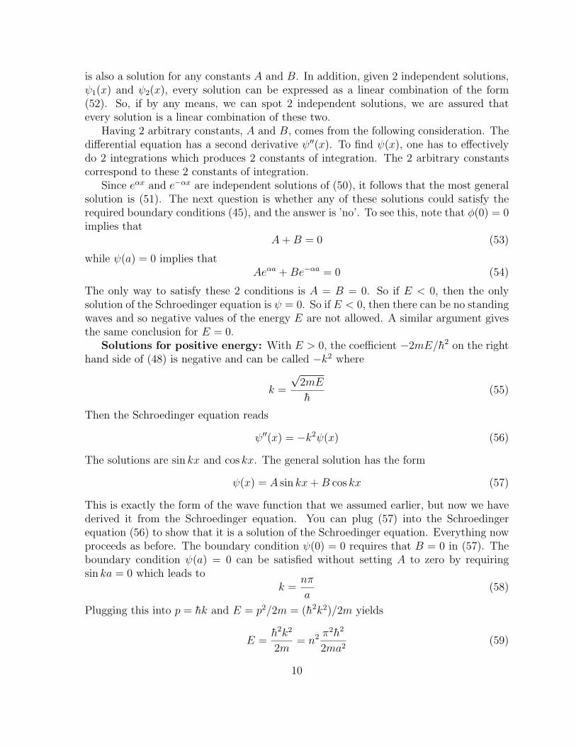
Figure 5: Probability density of a particle in the ground state of a rigid box.

which is sketched in Figure 5 (see also Fig. 7.6).(b) The most probable value, xmp, is the value of x for which |ψ(x)|2 is a maximum.

From Figure 7.6, this is seen to be

xmp = a/2 (69)

(c) The probability of finding the particle in any small interval from x to x + ∆x isgiven by (61) as

P (between x and x+∆x) ≈ |ψ(x)|2∆x (70)

Thus,

P (0.50a ≤ x ≤ 0.51a) ≈ |ψ(x = 0.50a)|2∆x =2

asin2

(

π

2

)

× 0.01a = 0.02 = 2% (71)

(e) The average result if we measure the position many times (always with the particlein the same state) is

〈x〉 =∫ a

0x|ψ(x)|2dx (72)

The average value 〈x〉 is called the expectation value of x. It is the average valueexpected after many measurements. For the ground state

〈x〉 =2

a

∫ a

0x sin2

(

πx

a

)

dx (73)

=a

2(74)

For the ground state of a particle in a box, the most probable position xmp and the meanposition 〈x〉 are the same, but this is not always the case as we shall see.

Expectation ValuesIn Example 7.2 we introduced the notation of the expectation value 〈x〉 of x. This

is not the value of x expected in any one measurement; rather it is the average value

12

expected if we repeat the measurement many times (always with the system in the samestate).

A quantity x can take various values with different probabilities. x could be a contin-uous or a discrete variable. Let us first consider the discrete case: Suppose the possibleresults of the measurement are x1, x2, ..., xi, ... and that these results occur with proba-bilities P1, P2, ..., Pi, ... If a large number N of statistically independent measurementsare made, the number of measurements resulting in the value xi will be ni = Pi ·N , i.e.,Pi = ni/N is the fraction of the measurements that yield the value xi. The average valueof x is the sum of all the results of all the measurements divided by the total number N .Since ni of the measurements produce the value xi, this sum of all the measurements is∑

i nixi, and the average value is

〈x〉 =1

N

∑

i

nixi (75)

=∑

i

ni

Nxi (76)

=∑

i

Pixi (77)

If x is a continuous variable, the probability Pi is replaced with a probability incrementp(x)dx, where p(x) is the probability density. For example, if x is the position of aquantum particle, p(x)dx = |ψ(x)|2. Then we get

〈x〉 =∑

i

Pixi → 〈x〉 =∫

xp(x)dx (78)

More generally, if we measure x2 or x3 or any function f(x), we can repeat the sameargument, simply replacing x with f(x), and conclude that

〈f(x)〉 =∫

f(x)p(x)dx (79)

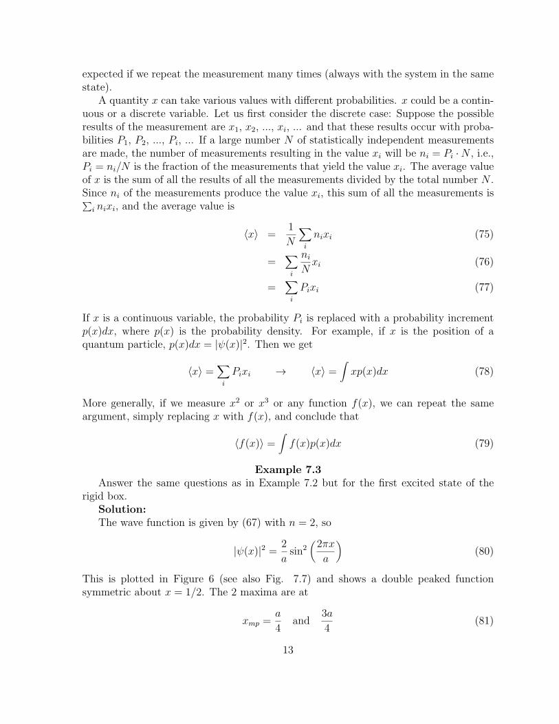
Example 7.3Answer the same questions as in Example 7.2 but for the first excited state of the

rigid box.Solution:The wave function is given by (67) with n = 2, so

|ψ(x)|2 = 2

asin2

(

2πx

a

)

(80)

This is plotted in Figure 6 (see also Fig. 7.7) and shows a double peaked functionsymmetric about x = 1/2. The 2 maxima are at

xmp =a

4and

3a

4(81)

13

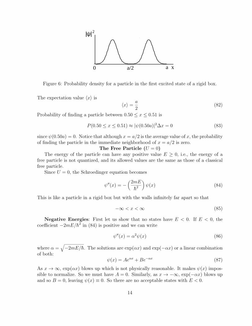
a

2

0 a/2

|ψ|

x

Figure 6: Probability density for a particle in the first excited state of a rigid box.

The expectation value 〈x〉 is〈x〉 = a

2(82)

Probability of finding a particle between 0.50 ≤ x ≤ 0.51 is

P (0.50 ≤ x ≤ 0.51) ≈ |ψ(0.50a)|2∆x = 0 (83)

since ψ(0.50a) = 0. Notice that although x = a/2 is the average value of x, the probabilityof finding the particle in the immediate neighborhood of x = a/2 is zero.

The Free Particle (U = 0)The energy of the particle can have any positive value E ≥ 0, i.e., the energy of a

free particle is not quantized, and its allowed values are the same as those of a classicalfree particle.

Since U = 0, the Schroedinger equation becomes

ψ′′(x) = −(

2mE

h̄2

)

ψ(x) (84)

This is like a particle in a rigid box but with the walls infinitely far apart so that

−∞ < x <∞ (85)

Negative Energies: First let us show that no states have E < 0. If E < 0, thecoefficient −2mE/h̄2 in (84) is positive and we can write

ψ′′(x) = α2ψ(x) (86)

where α =√

−2mE/h̄. The solutions are exp(αx) and exp(−αx) or a linear combinationof both:

ψ(x) = Aeαx + Be−αx (87)

As x → ∞, exp(αx) blows up which is not physically reasonable. It makes ψ(x) impos-sible to normalize. So we must have A = 0. Similarly, as x → −∞, exp(−αx) blows upand so B = 0, leaving ψ(x) ≡ 0. So there are no acceptable states with E < 0.

14

An acceptable wave function ψ(x) must not blow up as x → ±∞. This is anotherexample of a boundary condition, since the points x = ±∞ are the boundaries of thesystem.

Nonnegative Energies: Now consider E ≥ 0. The Schroedinger equation becomes

ψ′′(x) = −(

2mE

h̄2

)

ψ(x) = −k2ψ(x) (88)

where

k =

√2mE

h̄(89)

As before, the general solution is

ψ(x) = A sin kx+B cos kx (90)

Note that neither sin kx nor cos kx blow up as x→ ±∞. For any value of k, the function(90) is an acceptable solution for any value of A and B. Since we can have any value ofk, the allowed energies are continuous and are in the range 0 ≤ E < ∞. So the energyof a free particle is not quantized. Only when the particle is confined in some way is itsenergy quantized.

The positive energy wave functions are right and left moving waves. To see this, use

sin kx =eikx − e−ikx

2iand cos kx =

eikx + e−ikx

2(91)

to rewrite ψ(x) asψ(x) = Ceikx +De−ikx (92)

where C and D are arbitrary constants. The full, time-dependent wave function Ψ(x, t)for the spatial wave function in (92) is

Ψ(x, t) = ψ(x)e−iωt = Cei(kx−ωt) +De−i(kx−ωt) (93)

This is a superposition of 2 traveling waves, one moving to the right (first term withcoefficient C) and the other moving to the left (second term with coefficient D). Thismeans that if both C and D are nonzero, the wave function is a superposition of bothmomenta, going in the right and left directions.

The Nonrigid BoxRecall that for a rigid box

U(x) =

{

0 for 0 ≤ x ≤ a∞ for x < 0 and x > a

(94)

Here we consider a potential U <∞ for x < 0 and x > a. This means a finite amount ofenergy is needed to remove a particle from the box.

U(x) =

{

0 for 0 ≤ x ≤ aU0 for x < 0 and x > a

(95)

15

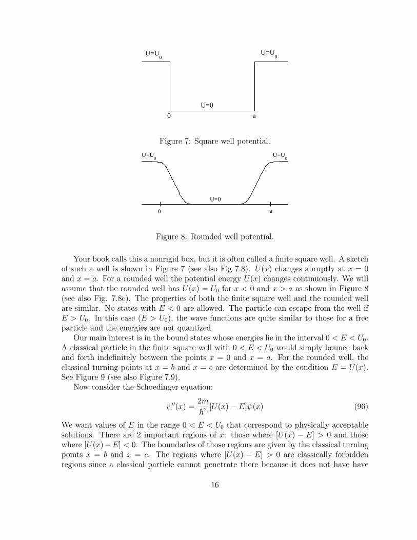
U=0

0U=U

0

0 a

U=U

Figure 7: Square well potential.

a

0U=U

0

U=0

0

U=U

Figure 8: Rounded well potential.

Your book calls this a nonrigid box, but it is often called a finite square well. A sketchof such a well is shown in Figure 7 (see also Fig 7.8). U(x) changes abruptly at x = 0and x = a. For a rounded well the potential energy U(x) changes continuously. We willassume that the rounded well has U(x) = U0 for x < 0 and x > a as shown in Figure 8(see also Fig. 7.8c). The properties of both the finite square well and the rounded wellare similar. No states with E < 0 are allowed. The particle can escape from the well ifE > U0. In this case (E > U0), the wave functions are quite similar to those for a freeparticle and the energies are not quantized.

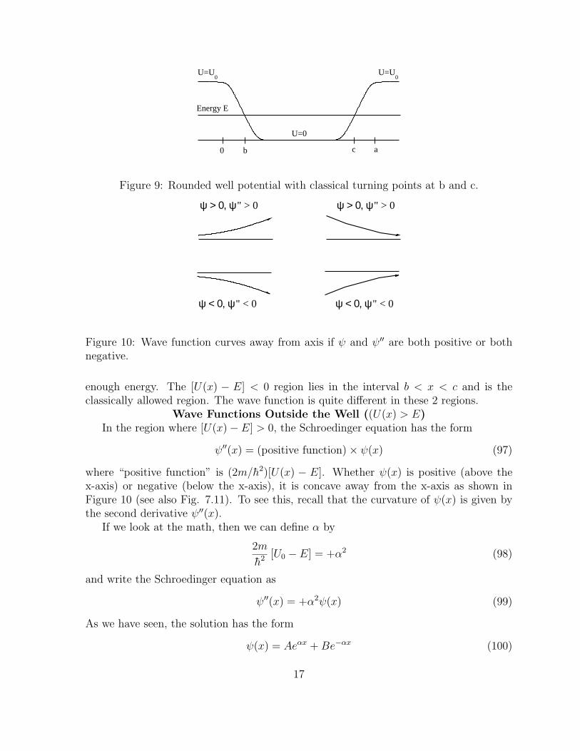
Our main interest is in the bound states whose energies lie in the interval 0 < E < U0.A classical particle in the finite square well with 0 < E < U0 would simply bounce backand forth indefinitely between the points x = 0 and x = a. For the rounded well, theclassical turning points at x = b and x = c are determined by the condition E = U(x).See Figure 9 (see also Figure 7.9).

Now consider the Schoedinger equation:

ψ′′(x) =2m

h̄2[U(x)− E]ψ(x) (96)

We want values of E in the range 0 < E < U0 that correspond to physically acceptablesolutions. There are 2 important regions of x: those where [U(x) − E] > 0 and thosewhere [U(x)−E] < 0. The boundaries of those regions are given by the classical turningpoints x = b and x = c. The regions where [U(x) − E] > 0 are classically forbiddenregions since a classical particle cannot penetrate there because it does not have have

16

a

0U=U

0

U=0

Energy E

b0 c

U=U

Figure 9: Rounded well potential with classical turning points at b and c.

" > 0

ψ < 0, ψ" < 0ψ < 0, ψ" < 0

ψ > 0, ψ" > 0ψ > 0, ψ

Figure 10: Wave function curves away from axis if ψ and ψ′′ are both positive or bothnegative.

enough energy. The [U(x) − E] < 0 region lies in the interval b < x < c and is theclassically allowed region. The wave function is quite different in these 2 regions.

Wave Functions Outside the Well ((U(x) > E)In the region where [U(x)− E] > 0, the Schroedinger equation has the form

ψ′′(x) = (positive function)× ψ(x) (97)

where “positive function” is (2m/h̄2)[U(x) − E]. Whether ψ(x) is positive (above thex-axis) or negative (below the x-axis), it is concave away from the x-axis as shown inFigure 10 (see also Fig. 7.11). To see this, recall that the curvature of ψ(x) is given bythe second derivative ψ′′(x).

If we look at the math, then we can define α by

2m

h̄2[U0 − E] = +α2 (98)

and write the Schroedinger equation as

ψ′′(x) = +α2ψ(x) (99)

As we have seen, the solution has the form

ψ(x) = Aeαx + Be−αx (100)

17

ψ < 0, ψψ > 0, ψ" < 0 " > 0

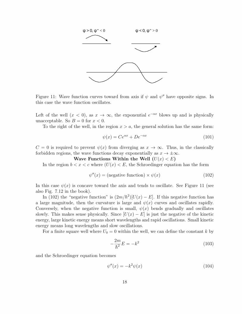
Figure 11: Wave function curves toward from axis if ψ and ψ′′ have opposite signs. Inthis case the wave function oscillates.

Left of the well (x < 0), as x → ∞, the exponential e−αx blows up and is physicallyunacceptable. So B = 0 for x < 0.

To the right of the well, in the region x > a, the general solution has the same form:

ψ(x) = Ceαx +De−αx (101)

C = 0 is required to prevent ψ(x) from diverging as x → ∞. Thus, in the classicallyforbidden regions, the wave functions decay exponentially as x→ ±∞.

Wave Functions Within the Well (U(x) < E)In the region b < x < c where (U(x) < E, the Schroedinger equation has the form

ψ′′(x) = (negative function)× ψ(x) (102)

In this case ψ(x) is concave toward the axis and tends to oscillate. See Figure 11 (seealso Fig. 7.12 in the book).

In (102) the “negative function” is (2m/h̄2)[U(x)− E]. If this negative function hasa large magnitude, then the curvature is large and ψ(x) curves and oscillates rapidly.Conversely, when the negative function is small, ψ(x) bends gradually and oscillatesslowly. This makes sense physically. Since [U(x)− E] is just the negative of the kineticenergy, large kinetic energy means short wavelengths and rapid oscillations. Small kineticenergy means long wavelengths and slow oscillations.

For a finite square well where U0 = 0 within the well, we can define the constant k by

−2m

h̄2E = −k2 (103)

and the Schroedinger equation becomes

ψ′′(x) = −k2ψ(x) (104)

18

The most general solution is

ψ(x) = F sin kx+G cos kx (105)

Solving for the allowed energies is rather messy. It involves starting with the generalsolutions and using the conditions that ψ(x) and ψ′(x) must be continuous at the edgesof the well to solve for the coefficents A, D, F , and G (we already know B = C = 0).There is no simple analytic solution to this problem and you have to use a computer toobtain a numerical solution.

Searching for Allowed EnergiesAcceptable solutions come from matching the solutions from various regions so that

the wave functions and their slopes are continuous at the boundaries between the regions.We do not want ψ(x) to diverge as x→ ±∞. For example, ψ(x) = Aeαx is well behavedfor x < 0 but blows up as x→ ∞. Go through Figures 7.13 to 7.16 for the rounded well.

Acceptable solutions for the finite square well are compared to those for the infinitesquare well in Figure 7.17. The ground state of the infinite square well fits exactly halfan oscillation while that of the finite well fits somewhat less than half an oscillation.The second function (first excited state) has one complete oscillation in the infinite wellwhile the finite well has just less than one oscillation. The wave function leaks a littleoutside the finite well. More wiggles mean higher kinetic energy, or more curvature meanshigher energy. Just look at the term with the second derivative with respect to x in theSchroedinger equation to see this. So the energy of each level of the finite square well isslightly lower than that of the corresponding level in the infinite well.

Notice that the ground-state wave function for any finite well has no nodes. A nodeis where the wave function goes to zero. The second level (first excited state) has onenode. The nth level has n − 1 nodes. More nodes correspond to higher energies sincehigher energy corresponds to a wave function that oscillates more quickly.

Note that the wave functions of the finite well are nonzero outside the well in theclassically forbidden region. The particle is bound inside or close to the potential well.Unlike a classical particle, there is a definite nonzero probability of finding the particle inthe classically forbidden regions. The ability of the quantum wave function to penetrateinto classically forbidden regions has important consequences like tunneling.

For the finite well, when E reaches U0, there are no more bound states and the particleis no longer confined. The number of bound states depends on the well depth U0 andwidth a, but is always finite.

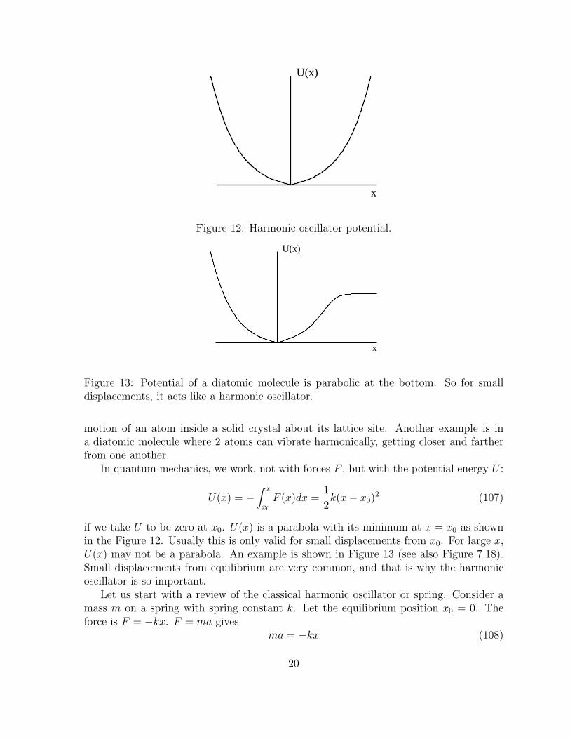
The Simple Harmonic Oscillator (SHO)Familiar classical examples of a harmonic oscillator are a mass suspended from an

ideal spring and a pendulum oscillating with a small amplitude. If a particle is displacedfrom its stable equilibrium position, x0, there is a restoring force pushing it back towardits equilibrium position:

F (x) = −k(x− x0) (106)

So a particle slightly displaced from equilibrium will oscillate harmonically about itsequilibrium position. A microscopic example of a quantum harmonic oscillator is the

19

x

U(x)

Figure 12: Harmonic oscillator potential.

U(x)

x

Figure 13: Potential of a diatomic molecule is parabolic at the bottom. So for smalldisplacements, it acts like a harmonic oscillator.

motion of an atom inside a solid crystal about its lattice site. Another example is ina diatomic molecule where 2 atoms can vibrate harmonically, getting closer and fartherfrom one another.

In quantum mechanics, we work, not with forces F , but with the potential energy U :

U(x) = −∫ x

x0

F (x)dx =1

2k(x− x0)

2 (107)

if we take U to be zero at x0. U(x) is a parabola with its minimum at x = x0 as shownin the Figure 12. Usually this is only valid for small displacements from x0. For large x,U(x) may not be a parabola. An example is shown in Figure 13 (see also Figure 7.18).Small displacements from equilibrium are very common, and that is why the harmonicoscillator is so important.

Let us start with a review of the classical harmonic oscillator or spring. Consider amass m on a spring with spring constant k. Let the equilibrium position x0 = 0. Theforce is F = −kx. F = ma gives

ma = −kx (108)

20

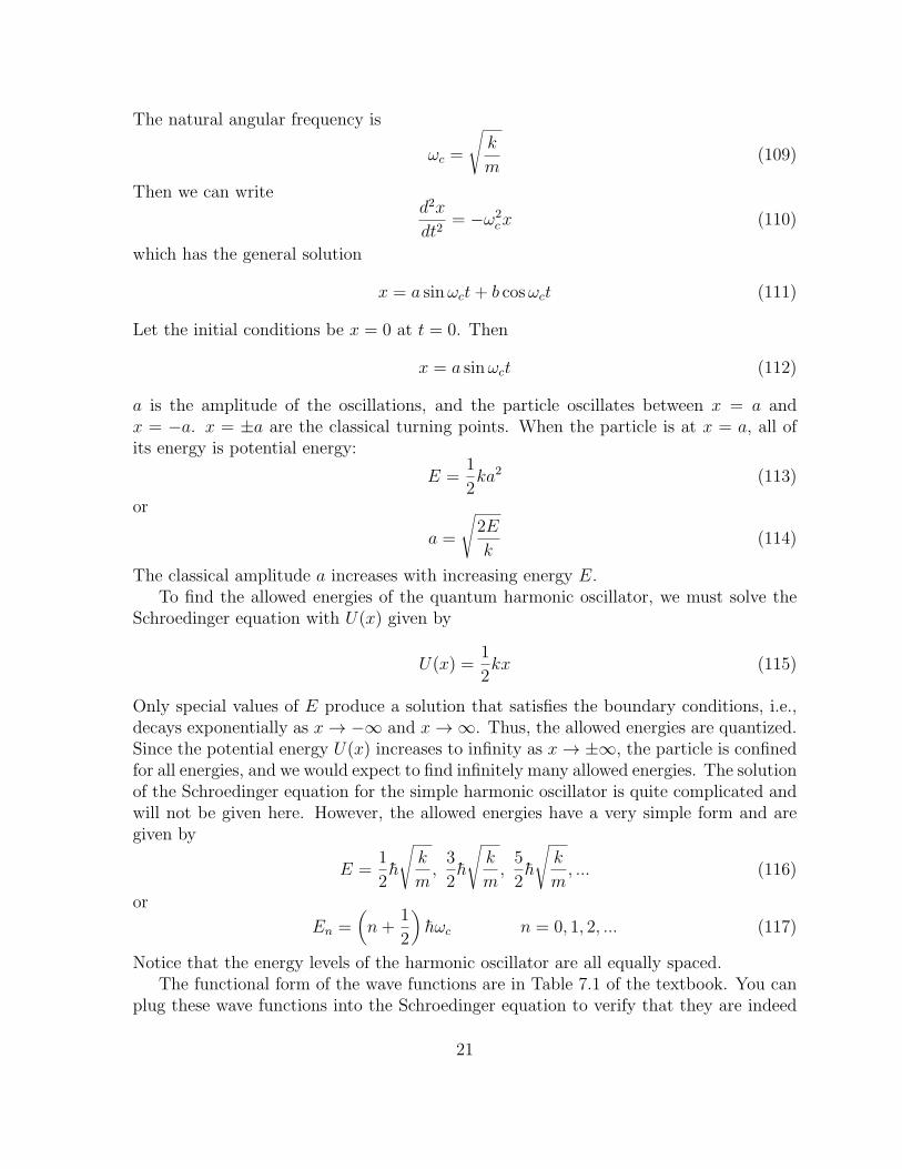
The natural angular frequency is

ωc =

√

k

m(109)

Then we can writed2x

dt2= −ω2

cx (110)

which has the general solution

x = a sinωct+ b cosωct (111)

Let the initial conditions be x = 0 at t = 0. Then

x = a sinωct (112)

a is the amplitude of the oscillations, and the particle oscillates between x = a andx = −a. x = ±a are the classical turning points. When the particle is at x = a, all ofits energy is potential energy:

E =1

2ka2 (113)

or

a =

√

2E

k(114)

The classical amplitude a increases with increasing energy E.To find the allowed energies of the quantum harmonic oscillator, we must solve the

Schroedinger equation with U(x) given by

U(x) =1

2kx (115)

Only special values of E produce a solution that satisfies the boundary conditions, i.e.,decays exponentially as x→ −∞ and x→ ∞. Thus, the allowed energies are quantized.Since the potential energy U(x) increases to infinity as x→ ±∞, the particle is confinedfor all energies, and we would expect to find infinitely many allowed energies. The solutionof the Schroedinger equation for the simple harmonic oscillator is quite complicated andwill not be given here. However, the allowed energies have a very simple form and aregiven by

E =1

2h̄

√

k

m,3

2h̄

√

k

m,5

2h̄

√

k

m, ... (116)

or

En =(

n+1

2

)

h̄ωc n = 0, 1, 2, ... (117)

Notice that the energy levels of the harmonic oscillator are all equally spaced.The functional form of the wave functions are in Table 7.1 of the textbook. You can

plug these wave functions into the Schroedinger equation to verify that they are indeed

21

U(x)=0

xx

E

U(x) = U

L

x0 1

0

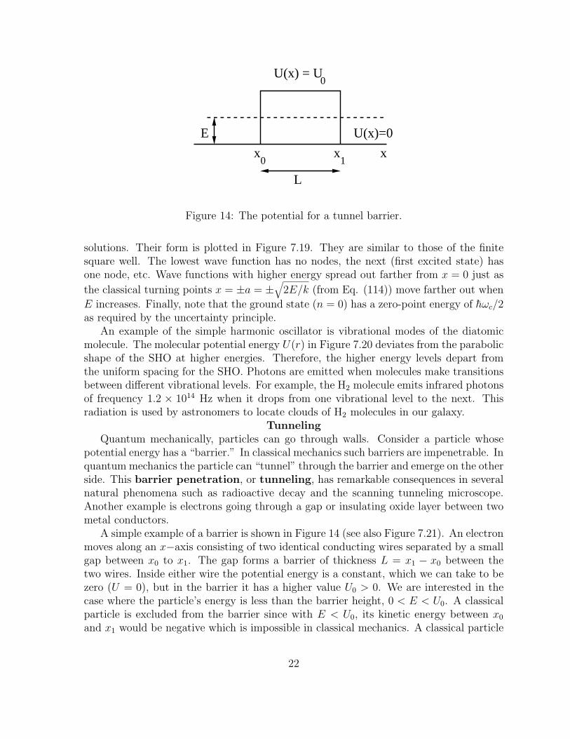
Figure 14: The potential for a tunnel barrier.

solutions. Their form is plotted in Figure 7.19. They are similar to those of the finitesquare well. The lowest wave function has no nodes, the next (first excited state) hasone node, etc. Wave functions with higher energy spread out farther from x = 0 just as

the classical turning points x = ±a = ±√

2E/k (from Eq. (114)) move farther out when

E increases. Finally, note that the ground state (n = 0) has a zero-point energy of h̄ωc/2as required by the uncertainty principle.

An example of the simple harmonic oscillator is vibrational modes of the diatomicmolecule. The molecular potential energy U(r) in Figure 7.20 deviates from the parabolicshape of the SHO at higher energies. Therefore, the higher energy levels depart fromthe uniform spacing for the SHO. Photons are emitted when molecules make transitionsbetween different vibrational levels. For example, the H2 molecule emits infrared photonsof frequency 1.2 × 1014 Hz when it drops from one vibrational level to the next. Thisradiation is used by astronomers to locate clouds of H2 molecules in our galaxy.

TunnelingQuantum mechanically, particles can go through walls. Consider a particle whose

potential energy has a “barrier.” In classical mechanics such barriers are impenetrable. Inquantum mechanics the particle can “tunnel” through the barrier and emerge on the otherside. This barrier penetration, or tunneling, has remarkable consequences in severalnatural phenomena such as radioactive decay and the scanning tunneling microscope.Another example is electrons going through a gap or insulating oxide layer between twometal conductors.

A simple example of a barrier is shown in Figure 14 (see also Figure 7.21). An electronmoves along an x−axis consisting of two identical conducting wires separated by a smallgap between x0 to x1. The gap forms a barrier of thickness L = x1 − x0 between thetwo wires. Inside either wire the potential energy is a constant, which we can take to bezero (U = 0), but in the barrier it has a higher value U0 > 0. We are interested in thecase where the particle’s energy is less than the barrier height, 0 < E < U0. A classicalparticle is excluded from the barrier since with E < U0, its kinetic energy between x0and x1 would be negative which is impossible in classical mechanics. A classical particle

22

would be reflected from the barrier.Now let us see what would happen quantum mechanically. Consider first a barrier

whose length L is infinite as shown in Figure 7.22. The potential energy is a step function.It is like a square well with just the right wall of the well. Suppose the step occurs atx = x0. To the left of x0, the kinetic energy K = (E − U) of a particle is positive andψ(x) is an oscillating sinusoidal wave. To the right of x0, (E − U) is negative and ψ(x)is a decreasing exponential with the form

ψ(x) = Be−αx (118)

where (see Eq. (98))

α =

√

2m(U0 − E)

h̄2(119)

The quantum particle has a nonzero probability of being found in the classically forbiddenregion where E − U is negative.

In the case of the infintely long barrier, ψ(x) goes steadily to zero as x increases.But if the barrier has a finite length, there is a finite probability that the particle canbe found on the other side of the barrier. Suppose the barrier extends from x0 to x1.The situation is shown in Figure 7.23. ψ(x) is sinusoidal (with amplitude AL) to the leftof x0, and decays exponentially within the barrier (x0 < x < x1). The barrier stops atx1, and (E − U) > 0 for x > x1. Therefore, before ψ(x) has decayed to zero, it startsoscillating again with amplitude AR to the right of the barrier.

The probability that the particle with E < U0 will tunnel through the barrier andemerge on the other side is

P ≈ e−2αL (120)

To see where this comes from, consider

ψ(L) ∼ e−αL

P = |ψ|2 ∼ e−2αL

where α is given by Eq. (119).The probability that a quantum particle will tunnel through the classically impene-

trable barrier depends on α and L, the thickness of the barrier. In many applications theproduct αL is very large and the probability (120) is therefore very small. Nevertheless,if the particle keeps trying and keeps bumping against the barrier, it will eventually passthrough it.

A modern application of quantum tunneling is the scanning tunneling microscope(STM). A tiny tip is placed a little ways above the conducting surface of the sample andelectrons are fired at the surface from the tip. This stream of electrons is an electriccurrent. By measuring the current, we can obtain information about the topography ofthe surface.

Example 7.5

23

Consider two identical conducting wires, lying on the x axis and separated by an airgap of thickness L = 1 nm, i.e., a few atomic diameters). An electron that is movinginside either conductor has U = 0, but in the gap U0 > 0. Thus the gap is the barrier inFigure 7.21. The electron approaches the barrier from the left with energy E such thatU0 − E = 1 eV, i.e., the electron’s energy is 1 eV below the top of the barrier. Whatis the probability that the electron will emerge on the other side of the barrier? Howdifferent would this be if the barrier were twice as wide?

Answer: The required probability is given by Eq. (120) with

α =

√

2m (U0 − E)

h̄

=

√

2mc2 (U0 − E)

h̄c

≈√

2× (5× 105 eV)× (1 eV)

197 eV − nm≈ 5.1 nm

Thus αL = 5.1 and the transmission probability is P = e−2αL = e−10.2 = 3.7 × 10−5

or about 0.004%. This probability is not large, but if we shoot enough electrons at thebarrier, some are bound to get through. If we double L, this will give a transmissionprobability

P ′ = e−4αL = e−20.4 = 1.4× 10−9 (121)

This is a dramatically smaller result. This is worse than your chance of winning thelottery. This illustrates the extreme sensitivity of the transmission probability to thewidth of the gap. So in STM, small changes in separation between the tip and thesurface would produce big changes in tunneling current. These changes would come fromthe hills and valleys or bumps in the surface. In fact, the tunneling current of the STMis held constant by having the tip stay at a constant distance from the surface througha feedback mechanism, and the changing position of the tip gives us the topography ofthe surface. See Chapter 14 for more information on how an STM works.

24