Embed Size (px)
Citation preview
January 2016 Urban Drainage and Flood Control District 7-i Urban Storm Drainage Criteria Manual Volume 1
Chapter 7 Street, Inlets, and Storm Drains Contents 1.0 Introduction ...................................................................................................................................... 1
1.1 Purpose and Background ........................................................................................................................... 1 1.2 Urban Stormwater Collection and Conveyance Systems .......................................................................... 1 1.3 System Components .................................................................................................................................. 2 1.4 Minor and Major Storms ........................................................................................................................... 2
2.0 Street Drainage ................................................................................................................................. 3 2.1 Street Function and Classification ............................................................................................................. 3 2.2 Design Considerations .............................................................................................................................. 4 2.3 Hydraulic Evaluation ................................................................................................................................ 6
2.3.1 Curb and Gutter ............................................................................................................................. 6 2.3.2 Swale Capacity ............................................................................................................................ 12
3.0 Inlets ................................................................................................................................................ 13 3.1 Inlet Function and Selection .................................................................................................................... 13 3.2 Design Considerations ............................................................................................................................ 13
3.2.1 Grate Inlets on a Continuous Grade ............................................................................................ 15 3.2.2 Curb-Opening Inlets on a Continuous Grade .............................................................................. 17 3.2.3 Combination Inlets on a Continuous Grade ................................................................................ 18 3.2.4 Slotted Inlets on a Continuous Grade .......................................................................................... 18 3.2.5 Grate Inlets in a Sump (UDFCD-CSU Model) ........................................................................... 19 3.2.6 Curb-Opening Inlets in a Sump (UDFCD-CSU Model) ............................................................. 20 3.2.7 Other Inlets in a Sump (Not Modeled in the UDFCD-CSU Study) ............................................ 24 3.2.8 Inlet Clogging ............................................................................................................................. 28 3.2.9 Nuisance Flows ........................................................................................................................... 29
3.3 Inlet Location and Spacing on Continuous Grades ................................................................................. 32 3.3.1 Design Considerations ................................................................................................................ 33 3.3.2 Design Procedure ........................................................................................................................ 33
4.0 Storm Drain Systems ..................................................................................................................... 34 4.1 Introduction ............................................................................................................................................. 34 4.2 Design Process, Considerations, and Constraints .................................................................................... 34 4.3 Storm Drain Hydrology—Peak Runoff Calculation ............................................................................... 36 4.4 Storm Drain Hydraulics (Gravity Flow in Circular Conduits) ................................................................ 36
4.4.1 Flow Equations and Storm Drain Sizing ..................................................................................... 36 4.4.2 Energy Grade Line and Head Losses .......................................................................................... 38
5.0 UD-Inlet Design Workbook ........................................................................................................... 48
6.0 Examples ......................................................................................................................................... 48 6.1 Example—Triangular Gutter Capacity ................................................................................................... 48 6.2 Example—Composite Gutter Capacity ................................................................................................... 49 6.3 Example—Composite Gutter Capacity – Major Storm Event ................................................................ 50 6.4 Example—V-Shaped Swale Capacity ..................................................................................................... 52 6.5 Example—V-Shaped Swale Design ........................................................................................................ 53 6.6 Example—Grate Inlet Capacity .............................................................................................................. 54 6.7 Example—Curb-Opening Inlet Capacity ................................................................................................ 56
7-ii Urban Drainage and Flood Control District January 2016 Urban Storm Drainage Criteria Manual Volume 1
6.8 Example—Design of a Network of Inlets Using UD-Inlet ..................................................................... 57
7.0 References ........................................................................................................................................ 61
Tables Table 7-1. Street classification for drainage purposes.................................................................................. 3 Table 7-2. Pavement encroachment and inundation standards for the minor storm .................................... 4 Table 7-3. Street inundation standards for the major (i.e., 100-year) storm ................................................ 5 Table 7-4. Allowable street cross-flow ........................................................................................................ 5 Table 7-5. Inlet selection considerations .................................................................................................... 13 Table 7-6. Splash-over velocity constants for various types of inlet grates ............................................... 16 Table 7-7. Coefficients for various inlets in sumps .................................................................................... 20 Table 7-8. Sump inlet discharge variables and coefficients ....................................................................... 26 Table 7-9. Clogging coefficient k for single and multiple units1 ............................................................... 28 Table 7-10. Nuisance flows: sources, problems and avoidance strategies ................................................. 31 Table 7-11. Bend loss and lateral loss coefficients (FHWA 2009) ............................................................ 44 Table 7-12. Head loss expansion coefficients in non-pressure flow (FHWA 2009) .................................. 45
Figures Figure 7-1. Gutter section with uniform cross slope .................................................................................... 7 Figure 7-2. Typical gutter section—composite cross slope ......................................................................... 8 Figure 7-3. Calculation of composite street section capacity: major storm ............................................... 10 Figure 7-4. Reduction factor for gutter flow (Guo 2000b) ......................................................................... 11 Figure 7-5. Typical v-shaped swale section ............................................................................................... 12 Figure 7-6. CDOT type r and Denver no. 14 interception capacity in sag ................................................. 21 Figure 7-7. CDOT type 13 interception capacity in a sump....................................................................... 23 Figure 7-8. Denver no. 16 interception capacity in sump .......................................................................... 24 Figure 7-9. Perspective views of grate and curb-opening inlets ................................................................ 27 Figure 7-10. Orifice calculation depths for curb-opening inlets ................................................................ 27 Figure 7-11. A pipe-manhole unit .............................................................................................................. 40 Figure 7-12. Hydraulic and energy grade lines .......................................................................................... 40 Figure 7-13. Bend loss coefficients ............................................................................................................ 46 Figure 7-14. Manhole benching methods ................................................................................................... 47 Figure 7-15. Angle of cone for pipe diameter changes .............................................................................. 47

Chapter 7 Streets, Inlets, & Storm Drains
January 2016 Urban Drainage and Flood Control District 7-1 Urban Storm Drainage Criteria Manual Volume 1
Photograph 7-1. From 2006 to 2011, hundreds of street and area inlet physical model tests were conducted at the CSU Hydraulics Laboratory, facilitating refinement of the HEC-22 methodology for inlets common to Colorado.
1.0 Introduction
1.1 Purpose and Background
The purpose of this chapter is to provide design guidance for stormwater collection and conveyance utilizing streets and storm drains. Procedures and equations are presented for the hydraulic design of street drainage, locating inlets and determining capture capacity, and sizing storm drains. This chapter also includes discussion on placing inlets to minimize the potential for icing. Examples are provided to illustrate the hydraulic design process and Excel workbook solutions accompany the hand calculations for most example problems.
The design procedures presented in this chapter are based upon fundamental hydrologic and hydraulic design concepts. It is assumed that the reader has an understanding of basic hydrology and hydraulics. A working knowledge of the Rational Method (Runoff chapter) and open channel hydraulics (Open Channels chapter) is particularly helpful. The design equations provided are well accepted and widely used. They are presented without derivations or detailed explanation but are properly referenced if the reader wishes to study their background. Inlet capacity, as presented in this chapter, is based on the FHWA Hydraulic Circular No. 22 (HEC-22) methodology (FHWA 2009), which was subsequently refined through a multi-jurisdictional partnership led by Urban Drainage and Flood Control (UDFCD), where hundreds of physical model tests of inlets commonly used in Colorado were performed at the Colorado State University (CSU) Hydraulics Laboratory. The physical model study is further detailed in technical papers available at www.udfcd.org. Additionally, UDFCD developed an inlet design tool, UD-Inlet, which incorporates the findings of the physical model. UD-Inlet is also available at www.udfcd.org.
1.2 Urban Stormwater Collection and Conveyance Systems
Urban stormwater collection and conveyance systems are critical components of the urban infrastructure. Proper design is essential to minimize flood damage and limit disruptions. The primary function of the system is to collect excess stormwater in street gutters, convey it through storm drains and along the street right-of-way, and discharge it into a detention basin, water quality best management practice (BMP), or the nearest receiving water body (FHWA 2009).
Proper and functional urban stormwater collection and conveyance systems:
Promote safe passage of vehicular traffic during minor storm events.
Maintain public safety and manage flooding during major storm events.
Minimize capital and maintenance costs of the system.

Streets, Inlets, & Storm Drains Chapter 7
7-2 Urban Drainage and Flood Control District January 2016 Urban Storm Drainage Criteria Manual Volume 1
Photograph 7-2. The capital costs of storm drain construction are high, emphasizing the importance of sound design.
1.3 System Components
Urban stormwater collection and conveyance systems are comprised of three primary components:
1. Street gutters and roadside swales,
2. Storm drain inlets, and
3. Storm drains (with appurtenances like manholes, junctions, etc.).
Street gutters and roadside swales collect runoff from the street (and adjacent areas) and convey the runoff to a storm drain inlet while maintaining the street’s level of service.
Inlets collect stormwater from streets and other land surfaces, transition the flow into storm drains, and provide maintenance access to the storm drain system. Storm drains convey stormwater in excess of street or swale capacity along the right-of-way and discharge into a stormwater management facility or directly into a receiving water body. In rare instances, stormwater pump stations (the design of which is not covered in this manual) are needed to lift and convey stormwater away from low-lying areas where gravity drainage is not possible. All of these components must be designed properly to achieve the objectives of the stormwater collection and conveyance system.
1.4 Minor and Major Storms
Rainfall events vary greatly in magnitude and frequency of occurrence. Major storms produce large flow rates but rarely occur. Minor storms produce smaller flow rates but occur more frequently. For economic reasons, stormwater collection and conveyance systems are not normally designed to pass the peak discharge during major storm events without some street flooding.
Stormwater collection and conveyance systems are designed to pass the peak discharge of the minor storm event (and smaller events) with minimal disruption to street traffic. To accomplish this, the spread and depth of water on the street is limited to some maximum mandated value during the minor storm event. Inlets must be strategically placed to pick up excess gutter or swale flow once the limiting allowable spread or depth of water is reached. The inlets collect and convey stormwater into storm drains, which are typically sized to pass the peak flow rate (minus the allowable street flow rate) from the minor storm without any surcharge. The magnitude of the minor storm is established by local ordinances or criteria, and the 2- or 5-year storms are commonly specified, based on many factors including street function, traffic load, vehicle speed, etc.
Local ordinances often also establish the return period for the major storm event, generally the 100-year storm (although it may be a lesser event for some retrofit projects with site constraints). During this event, runoff exceeds the minor storm allowable spread and depth in the street and capacity of storm drains, and storm drains may surcharge. Street flooding occurs, and traffic is disrupted as the street functions as an open channel. The designer must evaluate and design for the major event with regard to maintaining public safety and minimizing flood damages.
Chapter 7 Streets, Inlets, & Storm Drains
January 2016 Urban Drainage and Flood Control District 7-3 Urban Storm Drainage Criteria Manual Volume 1
2.0 Street Drainage
2.1 Street Function and Classification
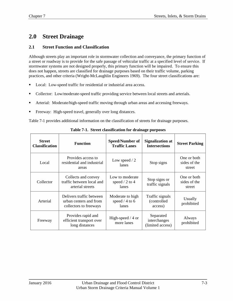
Although streets play an important role in stormwater collection and conveyance, the primary function of a street or roadway is to provide for the safe passage of vehicular traffic at a specified level of service. If stormwater systems are not designed properly, this primary function will be impaired. To ensure this does not happen, streets are classified for drainage purposes based on their traffic volume, parking practices, and other criteria (Wright-McLaughlin Engineers 1969). The four street classifications are:
Local: Low-speed traffic for residential or industrial area access.
Collector: Low/moderate-speed traffic providing service between local streets and arterials.
Arterial: Moderate/high-speed traffic moving through urban areas and accessing freeways.
Freeway: High-speed travel, generally over long distances.
Table 7-1 provides additional information on the classification of streets for drainage purposes.
Table 7-1. Street classification for drainage purposes
Street Classification Function Speed/Number of
Traffic Lanes Signalization at
Intersections Street Parking
Local Provides access to
residential and industrial areas
Low speed / 2 lanes Stop signs
One or both sides of the
street
Collector Collects and convey
traffic between local and arterial streets
Low to moderate speed / 2 to 4
lanes
Stop signs or traffic signals
One or both sides of the
street
Arterial Delivers traffic between urban centers and from collectors to freeways
Moderate to high speed / 4 to 6
lanes
Traffic signals (controlled
access)
Usually prohibited
Freeway Provides rapid and
efficient transport over long distances
High-speed / 4 or more lanes
Separated interchanges
(limited access)
Always prohibited
Streets, Inlets, & Storm Drains Chapter 7
7-4 Urban Drainage and Flood Control District January 2016 Urban Storm Drainage Criteria Manual Volume 1
Proper street drainage is essential to:
Maintain the street’s level of service.
Minimize danger and inconvenience to pedestrians during storm events (FHWA 1984).
Reduce potential for vehicular skidding and hydroplaning.
Maintain good visibility for drivers (by reducing splash and spray).
2.2 Design Considerations
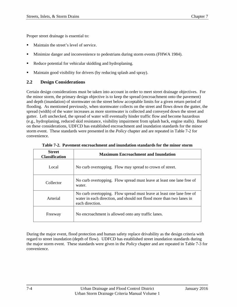
Certain design considerations must be taken into account in order to meet street drainage objectives. For the minor storm, the primary design objective is to keep the spread (encroachment onto the pavement) and depth (inundation) of stormwater on the street below acceptable limits for a given return period of flooding. As mentioned previously, when stormwater collects on the street and flows down the gutter, the spread (width) of the water increases as more stormwater is collected and conveyed down the street and gutter. Left unchecked, the spread of water will eventually hinder traffic flow and become hazardous (e.g., hydroplaning, reduced skid resistance, visibility impairment from splash back, engine stalls). Based on these considerations, UDFCD has established encroachment and inundation standards for the minor storm event. These standards were presented in the Policy chapter and are repeated in Table 7-2 for convenience.
Table 7-2. Pavement encroachment and inundation standards for the minor storm Street
Classification Maximum Encroachment and Inundation
Local No curb overtopping. Flow may spread to crown of street.
Collector No curb overtopping. Flow spread must leave at least one lane free of water.
Arterial No curb overtopping. Flow spread must leave at least one lane free of water in each direction, and should not flood more than two lanes in each direction.
Freeway No encroachment is allowed onto any traffic lanes.
During the major event, flood protection and human safety replace drivability as the design criteria with regard to street inundation (depth of flow). UDFCD has established street inundation standards during the major storm event. These standards were given in the Policy chapter and are repeated in Table 7-3 for convenience.

Chapter 7 Streets, Inlets, & Storm Drains
January 2016 Urban Drainage and Flood Control District 7-5 Urban Storm Drainage Criteria Manual Volume 1
Table 7-3. Street inundation standards for the major (i.e., 100-year) storm Street Classification Maximum Depth and Inundated Area
Local and Collector Residential dwellings and public, commercial, and industrial buildings should be no less than 12 inches above the 100-year flood at the ground line or lowest water entry of the building. The depth of water over the gutter flow line should not exceed 12 inches.
Arterial and Freeway Residential dwellings and public, commercial, and industrial buildings should be no less than 12 inches above the 100-year flood at the ground line or lowest water entry of the building. The depth of water should not exceed the street crown to allow operation of emergency vehicles. The depth of water over the gutter flow line should not exceed 12 inches.
Standards for the major storm and street cross-flows are also required. These standards apply at intersections, sump locations, and for culvert or bridge overtopping scenarios. The major storm needs to be assessed to determine the potential for flooding and public safety. Street cross-flows also need to be regulated for traffic flow and public safety reasons. These allowable street cross-flow standards were given in the Policy chapter and are repeated in Table 7-4 for convenience.
Table 7-4. Allowable street cross-flow Street Classification Initial Storm Flow Major (100-Year) Storm Flow
Local 6 inches of depth in cross-pan. 12 inches of depth above gutter flow line.
Collector Where cross-pans allowed, depth of flow should not exceed 6 inches.
12 inches of depth above gutter flow line.
Arterial/Freeway None. No cross-flow. Maximum depth at upstream gutter on road edge of 12 inches.
Once the allowable spread (pavement encroachment) and allowable depth (inundation) have been established for the minor storm, the placement of inlets can be determined. The inlets will remove some or all of the excess stormwater and thus reduce the spread and depth of flow. The placement of inlets is covered in Section 3.0. It should be noted that proper drainage design seeks to maximize the full allowable capacity of the street gutter in order to minimize the cost of inlets and storm drains.
Two additional design considerations are gutter geometry and street slope. Most urban streets incorporate curb and gutter sections. Various types exist, including spill shapes, catch shapes, curb heads, and mountable, a.k.a. “rollover” or “Hollywood” curbs. The shape is chosen for functional, cost, or aesthetic reasons and does not dramatically affect the hydraulic capacity. Swales are used along some semi-urban streets, and roadside ditches are common along rural streets. Cross-sectional geometry, longitudinal slopes and swale/ditch roughness values are important in determining hydraulic capacity and are covered in the next section.
Streets, Inlets, & Storm Drains Chapter 7
7-6 Urban Drainage and Flood Control District January 2016 Urban Storm Drainage Criteria Manual Volume 1
Street Hydraulic Capacity
This term typically refers to the capacity from the face of the curb to the crown (for the minor event).
Typically, the hydraulic computations necessary to determine street capacity and required inlet locations are performed independently for each side of the street. Additionally, flow and street geometry frequently differ from one side of a street to the other.
2.3 Hydraulic Evaluation
Hydraulic computations are performed to determine the capacity of roadside swales and street gutters and the encroachment of stormwater onto the street. The design discharge is based on the peak flow rate and usually is determined using the rational method (covered in the next two sections and in the Runoff Chapter). Although gutter, swale/ditch and street flows are unsteady and non-uniform, steady, uniform flow is assumed for the short time period of peak flow conditions.
2.3.1 Curb and Gutter
Both the longitudinal and cross (transverse) slope of a street are important in calculating hydraulic capacity. The capacity of the street increases as the longitudinal slope increases. UDFCD prescribes a minimum longitudinal slope of 0.4% for positive drainage (Wright-McLaughlin 1969). Public safety considerations limit the maximum allowable flow capacity of the gutter on steep slopes. The cross slope represents the slope from the street crown to the interface of the street and gutter, measured perpendicular to the direction of traffic. UDFCD recommends a minimum cross slope of 1% for positive drainage; however, a cross slope of 2% is more typical. Driver comfort and safety considerations limit the maximum cross slope. Use of standard curb and gutter sections typically produces a composite section with milder cross slopes for drive lanes and steeper cross slopes within the gutter width for increased flow capacity.
Each side of the street is evaluated independently. The hydraulic evaluation of street capacity includes the following steps: 1. Calculate the street capacity based upon the allowable spread for the minor storm as defined in
Table 7-2.
2. Calculate the street capacity based upon the allowable depth for the minor storm as defined in Table 7-2.
3. Calculate the allowable street capacity by multiplying the value calculated in step two (limited by depth) by the reduction factor provided in Figure 7-3. The lesser value (limited by allowable spread or by depth with a safety factor applied) is the allowable street capacity.
4. Repeat steps one through three for the major storm using criteria in Table 7-3.
Capacity When Gutter Cross Slope Equals Street Cross Slope (Not Typical) Streets with uniform cross slopes like that shown in Figure 7-1 are sometimes found in older urban areas. Since gutter flow is assumed to be uniform for design purposes, Manning’s equation is appropriate with a slight modification to account for the effects of a small hydraulic depth (A/T).

Chapter 7 Streets, Inlets, & Storm Drains
January 2016 Urban Drainage and Flood Control District 7-7 Urban Storm Drainage Criteria Manual Volume 1
Figure 7-1. Gutter section with uniform cross slope
For a triangular cross section as shown in Figure 7-1, Manning’s equation for gutter flow is written as:
3/82/13/52/13/2 56.08.1 TSSn
SARn
Q oxo == Equation 7-1
Where:
Q = calculated flow rate for the half-street (cfs) n = Manning’s roughness coefficient (0.016 for asphalt street with concrete gutter, 0.013 for concrete street and gutter) R = hydraulic radius of wetted cross section = A/P (ft)
A = cross-sectional area (ft2) P = wetted perimeter of cross section (ft) Sx = street cross slope (ft/ft) So = longitudinal slope (ft/ft) T = top width of flow spread (ft).
The flow depth can be found using:
xTSy = Equation 7-2
Where:
y = flow depth at the gutter flowline (ft). Note that the flow depth generally should not exceed the curb height during the minor storm based on Table 7-2. Manning’s equation can be written in terms of the flow depth, as:
382156.0 ySnS
Q Lx
= Equation 7-3
Streets, Inlets, & Storm Drains Chapter 7
7-8 Urban Drainage and Flood Control District January 2016 Urban Storm Drainage Criteria Manual Volume 1
The cross-sectional flow area, A, can be expressed as:
2
2TSA x= Equation 7-4
The gutter velocity at peak capacity may be found from continuity (V = Q/A). Triangular gutter cross-section calculations are illustrated in Example 7.1.
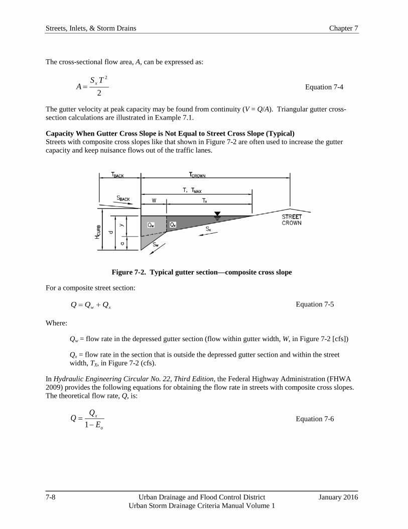
Capacity When Gutter Cross Slope is Not Equal to Street Cross Slope (Typical) Streets with composite cross slopes like that shown in Figure 7-2 are often used to increase the gutter capacity and keep nuisance flows out of the traffic lanes.
Figure 7-2. Typical gutter section—composite cross slope
For a composite street section:
xw QQQ += Equation 7-5
Where:
Qw = flow rate in the depressed gutter section (flow within gutter width, W, in Figure 7-2 [cfs])
Qx = flow rate in the section that is outside the depressed gutter section and within the street width, TX, in Figure 7-2 (cfs).
In Hydraulic Engineering Circular No. 22, Third Edition, the Federal Highway Administration (FHWA 2009) provides the following equations for obtaining the flow rate in streets with composite cross slopes. The theoretical flow rate, Q, is:
o
x
EQQ−
=1
Equation 7-6
Chapter 7 Streets, Inlets, & Storm Drains
January 2016 Urban Drainage and Flood Control District 7-9 Urban Storm Drainage Criteria Manual Volume 1
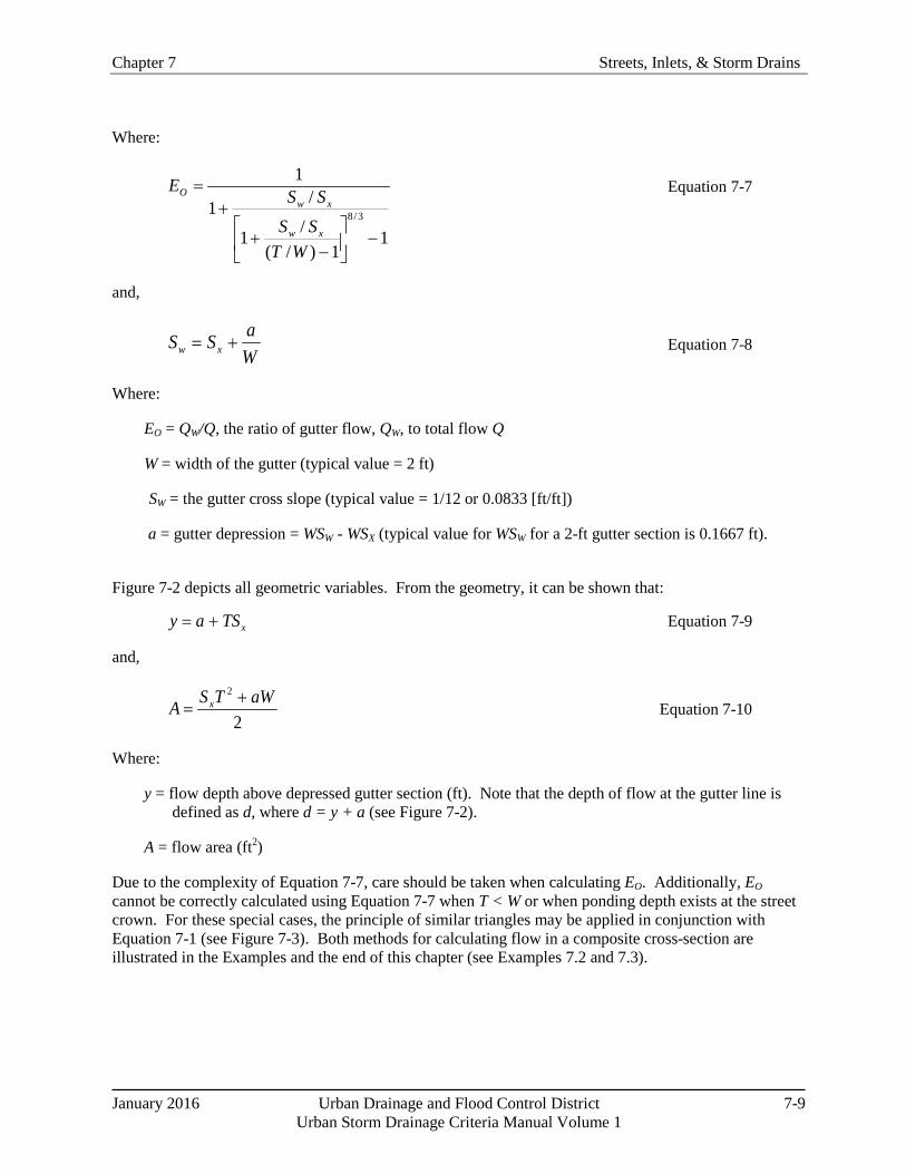
Where:
11)/(
/1
/1
1
3/8
−
−
+
+=
WTSSSSE
xw
xwO Equation 7-7
and,
WaSS xw += Equation 7-8
Where:
EO = QW/Q, the ratio of gutter flow, QW, to total flow Q
W = width of the gutter (typical value = 2 ft)
SW = the gutter cross slope (typical value = 1/12 or 0.0833 [ft/ft])
a = gutter depression = WSW - WSX (typical value for WSW for a 2-ft gutter section is 0.1667 ft).
Figure 7-2 depicts all geometric variables. From the geometry, it can be shown that:
xTSay += Equation 7-9
and,
2
2 aWTSA x += Equation 7-10
Where:
y = flow depth above depressed gutter section (ft). Note that the depth of flow at the gutter line is defined as d, where d = y + a (see Figure 7-2).
A = flow area (ft2)
Due to the complexity of Equation 7-7, care should be taken when calculating EO. Additionally, EO cannot be correctly calculated using Equation 7-7 when T < W or when ponding depth exists at the street crown. For these special cases, the principle of similar triangles may be applied in conjunction with Equation 7-1 (see Figure 7-3). Both methods for calculating flow in a composite cross-section are illustrated in the Examples and the end of this chapter (see Examples 7.2 and 7.3).

Streets, Inlets, & Storm Drains Chapter 7
7-10 Urban Drainage and Flood Control District January 2016 Urban Storm Drainage Criteria Manual Volume 1
Figure 7-3. Calculation of composite street section capacity: major storm
Allowable Capacity Stormwater flows along streets exert momentum forces on cars, pavement, and pedestrians. To limit the hazardous nature of large street flows, it is necessary to set limits on flow velocities and depths. As a result, the allowable half-street hydraulic capacity is determined as the lesser of:
TA QQ = Equation 7-11
or
dA QRQ = Equation 7-12
Where:
QA = allowable street hydraulic capacity (cfs)
QT = street hydraulic capacity where flow spread equals allowable spread (cfs)
R = reduction factor (allowable street and gutter flow for safety)
Qd = street hydraulic capacity where flow depth equals allowable depth (cfs).
There are two sets of safety reduction factors developed for the UDFCD region (Guo 2000b). One is for the minor event, and another is for the major event. Figure 7-4 shows that the safety reduction factor does not apply unless the street longitudinal slope is more than 1.5% for the major event and 2% for the minor event. The safety reduction factor, representing the fraction of calculated gutter flow at maximum depth

Chapter 7 Streets, Inlets, & Storm Drains
January 2016 Urban Drainage and Flood Control District 7-11 Urban Storm Drainage Criteria Manual Volume 1
that is used for the allowable design flow, decreases as longitudinal slope increases.
It is important for street drainage designs that the allowable street hydraulic capacity be used instead of the calculated gutter-full capacity. Where the accumulated stormwater amount on the street approaches the allowable capacity, a street inlet should be installed.
Figure 7-4. Reduction factor for gutter flow (Guo 2000b)

Streets, Inlets, & Storm Drains Chapter 7
7-12 Urban Drainage and Flood Control District January 2016 Urban Storm Drainage Criteria Manual Volume 1
2.3.2 Swale Capacity
Where curb and gutter are not used to contain flow, swales are frequently used to convey runoff and disconnect impervious areas. It is very important that swale depths and side slopes be shallow for safety and maintenance reasons. Street-side drainage swales are not the same as roadside ditches. Street-side drainage swales provide mild side slopes and are frequently designed to provide water quality enhancement. For purposes of disconnecting impervious area and reducing the overall volume of runoff, swales should be considered as collectors of initial runoff for transport to other larger means of conveyance. To be effective, they need to be limited to the velocity, depth, and cross-slope geometries considered acceptable.
Equation 7-1 can be used to calculate the flow rate in a V-section swale (using the appropriate roughness value for the swale lining) with an adjusted cross slope found using:
21
21
xx
xxx SS
SSS+
= Equation 7-13
Where:
Sx = adjusted side slope (ft/ft)
Sx1 = right side slope (ft/ft) Sx2 = left side slope (ft/ft).
Figure 7-5 shows the geometric variables, and Examples 7.4 and 7.5 show V-shaped swale calculations.
For safety reasons, paved swales should be designed such that the product of velocity and depth is no more than six for the minor storm and eight for the major storm.
For grass swales, refer to the Grass Swale Fact Sheet in the Urban Storm Drainage Criteria Manual (USDCM) Volume 3. During the 2-year event, grass swales designed for water quality should have a Froude number of no more than 0.5, a velocity that does not exceed 1.0 ft/s, and a depth that does not exceed 1.0 foot.
Note that the slope of a roadside ditch or swale can be different than the adjacent street. The hydraulic characteristics of the swale can therefore change from one location to another.
Figure 7-5. Typical v-shaped swale section

Chapter 7 Streets, Inlets, & Storm Drains
January 2016 Urban Drainage and Flood Control District 7-13 Urban Storm Drainage Criteria Manual Volume 1
Allowable Street Capacity
To a great degree, allowable street capacity dictates the placement of inlets. This term refers to the lesser of:
• Capacity determined by the allowable spread for the minor event
• Capacity determined by the allowable depth for the minor event, multiplied by a reduction factor
3.0 Inlets
3.1 Inlet Function and Selection
Inlets collect excess stormwater from the street, transition the flow into storm drains, and can provide maintenance access to the storm drain system. There are four major types of inlets: grate, curb opening, combination, and slotted (see Figure 7-11). Table 7-5 provides considerations in proper selection.
Table 7-5. Inlet selection considerations Inlet Type Applicable Setting Advantages Disadvantages
Grate Sumps and continuous grades (should be made bicycle safe)
Perform well over wide range of grades
Can become clogged Lose some capacity with increasing grade
Curb-opening Sumps and continuous grades (but not steep grades)
Do not clog easily Bicycle safe
Lose capacity with increasing grade
Combination Sumps and continuous grades (should be made bicycle safe)
High capacity Do not clog easily
More expensive than grate or curb-opening acting alone
Slotted Locations where sheet flow must be intercepted.
Intercept flow over wide section
Susceptible to clogging
3.2 Design Considerations
Frequently roadway geometry dictates the location of inlets. Inlets are placed at low points (sumps), median breaks, and at intersections. Additional inlets should be placed where the design peak flow on the street half is approaching the allowable capacity of the street half (see inset). Allowable street capacity will be exceeded and storm drains will be underutilized when inlets are not located properly or not designed for adequate capacity (Akan and Houghtalen 2002).
Inlets placed on continuous grades are generally designed to intercept only a portion of the gutter flow during the minor (design) storm (i.e. some flow bypasses to downgradient inlets). The effectiveness of the inlet is expressed as efficiency defined as:
QQE i= Equation 7-15
Where: E = inlet efficiency (fraction of gutter flow captured by inlet) Qi = intercepted flow rate (cfs) Q = total half-street flow rate (cfs).

Streets, Inlets, & Storm Drains Chapter 7
7-14 Urban Drainage and Flood Control District January 2016 Urban Storm Drainage Criteria Manual Volume 1
Bypass (or carryover) flow is not intercepted by the inlet. By definition,
ib QQQ −= Equation 7-16
Where:
Qb = bypass (or carryover) flow rate (cfs).
The ability of an inlet to intercept flow (i.e., hydraulic capacity) on a continuous grade increases to a degree with increasing gutter flow, but the capture efficiency decreases. In general, the inlet capacity depends upon:
The inlet type and geometry (length, width, curb opening, etc.),
The flow rate,
The longitudinal slope,
The cross (transverse) slope.
The capacity of an inlet varies with the type of inlet. For grate inlets, the capacity is largely dependent on the amount of water flowing over the grate, the grate configuration and spacing. For curb-opening inlets, the capacity is largely dependent on the length of the opening, street and gutter cross slope, and the flow depth at the curb. Local gutter depression at the curb opening will increase the capacity. Combination inlets on a continuous grade (i.e., not in a sump location) intercept up to 18% more than grate inlets alone and are much less likely to clog completely (CSU 2009). Slotted inlets function in a manner similar to curb-opening inlets (FHWA 2009).
Inlets in sumps operate as weirs at shallow ponding and as orifices as depth increases. A transition region exists between weir flow and orifice flow, much like a culvert. Grate inlets and slotted inlets have a higher tendency to clog with debris than do curb-openings inlets, so calculations should take that into account.
The hydraulic capacity of an inlet is dependent on the type of inlet (grate, curb opening, combination, or slotted) and the location (on a continuous grade or in a sump). The methodology for determination of hydraulic capacity of the various inlet types is described in the following sections.
(a) CDOT Type 13 grated inlet in combination configuration
(b) Denver No. 16 grated inlet in combination configuration
(c) CDOT Type R curb-opening
inlet Photograph 7-3. These three street inlets are the most commonly used in the UDFCD region. Their performance was tested for both on grade conditions and in sump conditions in a 1/3-scale physical model at CSU.
Chapter 7 Streets, Inlets, & Storm Drains
January 2016 Urban Drainage and Flood Control District 7-15 Urban Storm Drainage Criteria Manual Volume 1
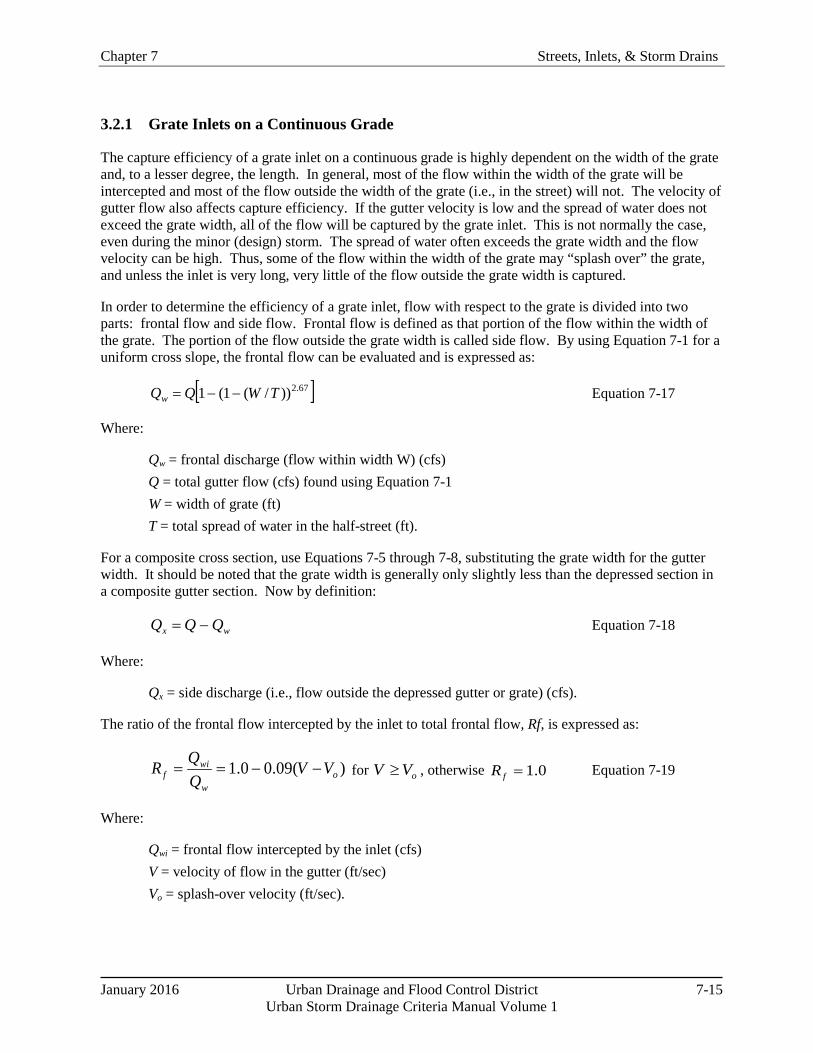
3.2.1 Grate Inlets on a Continuous Grade
The capture efficiency of a grate inlet on a continuous grade is highly dependent on the width of the grate and, to a lesser degree, the length. In general, most of the flow within the width of the grate will be intercepted and most of the flow outside the width of the grate (i.e., in the street) will not. The velocity of gutter flow also affects capture efficiency. If the gutter velocity is low and the spread of water does not exceed the grate width, all of the flow will be captured by the grate inlet. This is not normally the case, even during the minor (design) storm. The spread of water often exceeds the grate width and the flow velocity can be high. Thus, some of the flow within the width of the grate may “splash over” the grate, and unless the inlet is very long, very little of the flow outside the grate width is captured.
In order to determine the efficiency of a grate inlet, flow with respect to the grate is divided into two parts: frontal flow and side flow. Frontal flow is defined as that portion of the flow within the width of the grate. The portion of the flow outside the grate width is called side flow. By using Equation 7-1 for a uniform cross slope, the frontal flow can be evaluated and is expressed as:
[ ]67.2))/(1(1 TWQQw −−= Equation 7-17
Where:
Qw = frontal discharge (flow within width W) (cfs) Q = total gutter flow (cfs) found using Equation 7-1 W = width of grate (ft) T = total spread of water in the half-street (ft).
For a composite cross section, use Equations 7-5 through 7-8, substituting the grate width for the gutter width. It should be noted that the grate width is generally only slightly less than the depressed section in a composite gutter section. Now by definition:
wx QQQ −= Equation 7-18
Where:
Qx = side discharge (i.e., flow outside the depressed gutter or grate) (cfs).
The ratio of the frontal flow intercepted by the inlet to total frontal flow, Rf, is expressed as:
)(09.00.1 ow
wif VV
QQR −−== for oVV ≥ , otherwise 0.1=fR Equation 7-19
Where:
Qwi = frontal flow intercepted by the inlet (cfs) V = velocity of flow in the gutter (ft/sec) Vo = splash-over velocity (ft/sec).
Streets, Inlets, & Storm Drains Chapter 7
7-16 Urban Drainage and Flood Control District January 2016 Urban Storm Drainage Criteria Manual Volume 1
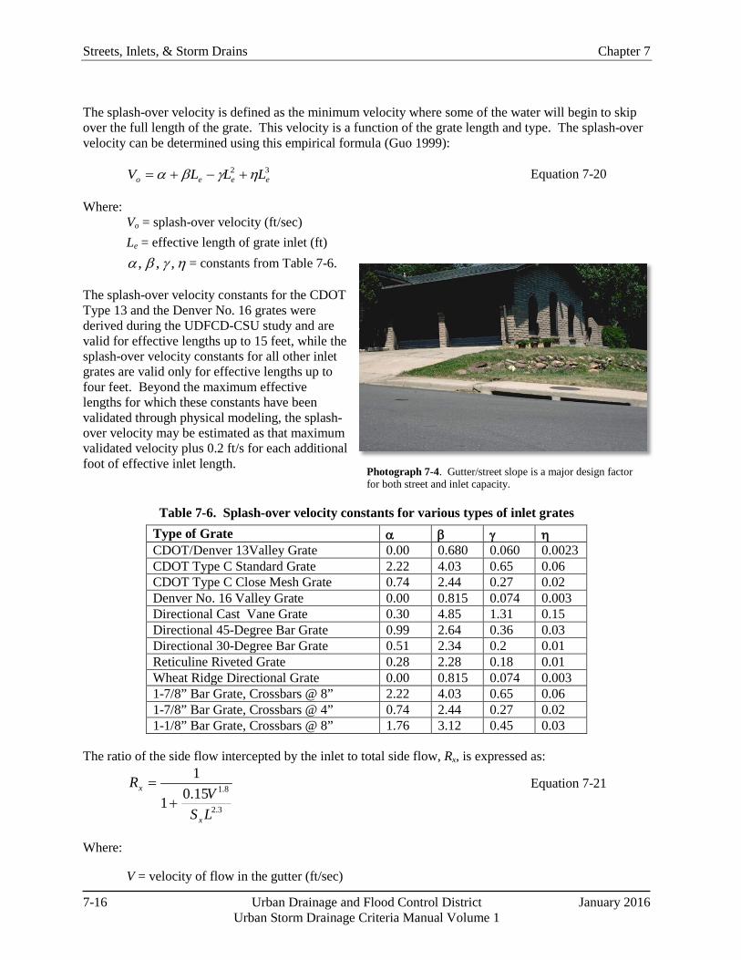
Photograph 7-4. Gutter/street slope is a major design factor for both street and inlet capacity.
The splash-over velocity is defined as the minimum velocity where some of the water will begin to skip over the full length of the grate. This velocity is a function of the grate length and type. The splash-over velocity can be determined using this empirical formula (Guo 1999):
32eeeo LLLV ηγβα +−+= Equation 7-20
Where: Vo = splash-over velocity (ft/sec) Le = effective length of grate inlet (ft)
ηγβα ,,, = constants from Table 7-6.
The splash-over velocity constants for the CDOT Type 13 and the Denver No. 16 grates were derived during the UDFCD-CSU study and are valid for effective lengths up to 15 feet, while the splash-over velocity constants for all other inlet grates are valid only for effective lengths up to four feet. Beyond the maximum effective lengths for which these constants have been validated through physical modeling, the splash-over velocity may be estimated as that maximum validated velocity plus 0.2 ft/s for each additional foot of effective inlet length.
Table 7-6. Splash-over velocity constants for various types of inlet grates
Type of Grate α β γ η CDOT/Denver 13Valley Grate 0.00 0.680 0.060 0.0023 CDOT Type C Standard Grate 2.22 4.03 0.65 0.06 CDOT Type C Close Mesh Grate 0.74 2.44 0.27 0.02 Denver No. 16 Valley Grate 0.00 0.815 0.074 0.003 Directional Cast Vane Grate 0.30 4.85 1.31 0.15 Directional 45-Degree Bar Grate 0.99 2.64 0.36 0.03 Directional 30-Degree Bar Grate 0.51 2.34 0.2 0.01 Reticuline Riveted Grate 0.28 2.28 0.18 0.01 Wheat Ridge Directional Grate 0.00 0.815 0.074 0.003 1-7/8” Bar Grate, Crossbars @ 8” 2.22 4.03 0.65 0.06 1-7/8” Bar Grate, Crossbars @ 4” 0.74 2.44 0.27 0.02 1-1/8” Bar Grate, Crossbars @ 8” 1.76 3.12 0.45 0.03
The ratio of the side flow intercepted by the inlet to total side flow, Rx, is expressed as:
3.2
8.115.01
1
LSV
R
x
x
+= Equation 7-21
Where:
V = velocity of flow in the gutter (ft/sec)

Chapter 7 Streets, Inlets, & Storm Drains
January 2016 Urban Drainage and Flood Control District 7-17 Urban Storm Drainage Criteria Manual Volume 1
L = length of grate (ft).
The capture efficiency, E, of the grate inlet may now be determined using:
( ) ( )QQRQQRE xxwf += Equation 7-22
Example 7.6 shows grate inlet capacity calculations.
3.2.2 Curb-Opening Inlets on a Continuous Grade
The capture efficiency of a curb-opening inlet is dependent on the length of the opening, the depth of flow at the gutter flow line, street cross slope and the longitudinal gutter slope (see Photograph 7-4). If the curb opening is long, the flow rate is low, and the longitudinal gutter slope is small, all of the flow will be captured by the inlet. It is generally uneconomical to install a curb opening long enough to capture all of the flow during the minor (design) storm. Thus, some water gets by the inlet, and the inlet efficiency needs to be determined.
The hydraulics of curb-opening inlets are less complicated than grate inlets. The efficiency, E, of a curb-opening inlet is calculated as:
( )[ ] 8.111 TLLE −−= for L < LT, otherwise E = 1.0 Equation 7-23
Where:
L = curb-opening length (ft) LT = curb-opening length required to capture 100% of gutter flow (ft).
For a curb-opening inlet in a uniform cross slope (see Figure 7-1), LT can be calculated as:
46.0058.051.0 138.0
=
xLT nS
SQL Equation 7-24
Where:
Q = total flow (cfs) SL = longitudinal street slope (ft/ft) Sx = street cross slope (ft/ft) n = Manning’s roughness coefficient.
But most curb-opening inlets are in a composite street section and many also have a localized depression, so LT should then be calculated as:
46.0058.051.0 138.0
=
eLT nS
SQL Equation 7-25
The equivalent cross slope, Se, can be determined from:

Streets, Inlets, & Storm Drains Chapter 7
7-18 Urban Drainage and Flood Control District January 2016 Urban Storm Drainage Criteria Manual Volume 1
Photograph 7-5. Inlets that are located in street vertical sag curves (sumps) are highly efficient.
olocal
xe EWaaSS )( +
+= Equation 7-26
Where:
a = gutter depression (as defined for Equation 7-8)
alocal = any additional local depression in the area of the inlet (typically specific to the type of inlet)
W = depressed gutter width as shown in Figure 7-2.
The ratio of the flow in the depressed section to total gutter flow, Eo, can be calculated from Equation 7-7. See Examples 7.6 and 7.7 for curb-opening inlet calculations.
3.2.3 Combination Inlets on a Continuous Grade
Combination inlets take advantage of the debris removal capabilities of a curb-opening inlet and the capture efficiency of a grate inlet. Combination inlets on a continuous grade (i.e., not in a sump location) intercept 18% more than grate inlets alone and are much less likely to clog completely (CSU 2009). A special case combination where the curb opening extends upstream of the grated section is called a sweeper inlet. The inlet capacity is enhanced by the additional upstream curb-opening length, and debris is intercepted there before it can clog the grate. The construction of sweeper inlets is more complicated and costly however, and they are not commonly seen in the UDFCD region. To calculate interception efficiency for a sweeper inlet, the upstream curb-opening efficiency is calculated first and then the interception efficiency for combination section based on the remaining street flow is added to it. To analyze this within UD-Inlet select user-defined combination, select a grate type, and check the sweeper configuration box.
3.2.4 Slotted Inlets on a Continuous Grade
Slotted inlets can be used in place of curb-opening inlets or can be used to intercept sheet flow that is crossing the pavement in an undesirable location. Unlike grate inlets, they have the advantage of intercepting flow over a wide section. They do not interfere with traffic operations and can be used on both curbed and uncurbed sections. Like grate inlets, they are susceptible to clogging.
Slotted inlets placed parallel to flow in the gutter flow line function like side-flow weirs, much like curb-opening inlets. The FHWA (1996) suggests the hydraulic capacity of slotted inlets closely corresponds to curb-opening inlets if the slot openings exceed 1.75 inches. Therefore, the equations developed for curb-opening inlets (Equations 7-23 through 7-26) are appropriate for those slotted inlets.
Chapter 7 Streets, Inlets, & Storm Drains
January 2016 Urban Drainage and Flood Control District 7-19 Urban Storm Drainage Criteria Manual Volume 1
3.2.5 Grate Inlets in a Sump (UDFCD-CSU Model)
All of the stormwater draining to a sump inlet must pass through an inlet grate or curb opening to enter the storm drain. This means that clogging due to debris can result not only in underutilized pipe conveyance, but also ponding of water on the surface. Surface ponding can be a nuisance or hazard. Therefore, the capacity of inlets in sumps must account for this clogging potential. Grate inlets acting alone are not recommended for this reason. Curb-opening and combination (including sweeper) inlets are more appropriate. In all sump inlet locations, consider the risk and required maintenance associated with a fully clogged condition and design the system accordingly. Photograph 7-5 shows a curb-opening inlet in a sump condition. At this location, if the inlet clogs, standing water will be limited to the elevation at the back of the walk.
The flow through a grated sump inlet varies with respect to depth and continuously changes from weir flow (at shallow depths) to mixed flow (at intermediate depths), and also orifice flow (at greater depths). For CDOT Type 13 grates and Denver No. 16 grates (the most common grated street inlets in the UDFCD region), from the UDFCD-CSU physical model study, the classic formulas for weir and orifice flow were modified with weir length and open area ratios specifically as:
2/3)2( DLWCNQ egwww += Equation 7-27
gDLWCNQ egooo 2= Equation 7-28
Where:
Qw = weir flow (cfs)
Qo = orifice flow (cfs)
Wg = grate width (ft)
Le = effective grate length after clogging (ft)
D = water depth at gutter flow line outside the local depression at the inlet (ft)
Nw = weir length reduction factor
No = orifice area reduction factor
Cw = weir discharge coefficient
Co = orifice discharge coefficient
The transient process between weir and orifice flows is termed mixed flow and is modeled as:
owmm QQCQ = Equation 7-29
Where:
Qm = mixed flow (cfs)
Cm = mixed flow coefficient
Streets, Inlets, & Storm Drains Chapter 7
7-20 Urban Drainage and Flood Control District January 2016 Urban Storm Drainage Criteria Manual Volume 1
The recommended values for the coefficients Nw, No, Cw, Cm, and Co are listed in Table 7-7.
In practice, for the given water depth, it is suggested that the interception capacity, Qi, for the sump grate be the smallest among the weir, orifice, and mixed flows as:
),,min( omwi QQQQ = Equation 7-30
3.2.6 Curb-Opening Inlets in a Sump (UDFCD-CSU Model)
Like a grate inlet, a curb-opening inlet operates under weir, orifice, or mixed flow. From the UDFCD-CSU physical model study, the HEC-22 procedure was found to overestimate the capacity of the CDOT Type R, the Denver No. 14, and other, similar curb-opening inlets for the minor storm event, and underestimate capacity for the major event. From the UDFCD-CSU study of these inlets, the interception capacity is based on the depression and opening geometry and can be estimated as:
2/3DLNCQ ewww = Equation 7-31
)5.0(2)( cceooo HDgHLNCQ −= Equation 7-32
Where:
Hc = height of the curb-opening throat (ft)
D = water depth at gutter flow line outside the local depression at the inlet (ft).
The recommended values for the coefficients Nw, No, Cw, Cm, and Co are listed in Table 7-7. Once weir and orifice interception rates are calculated, Equations 7-29 and 7-30 must also be applied to curb-opening inlets in sag locations.
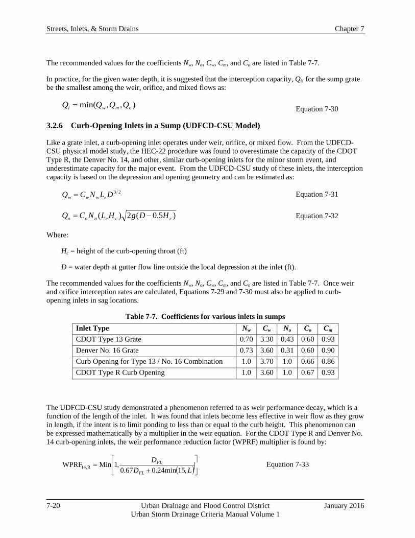
Table 7-7. Coefficients for various inlets in sumps Inlet Type Nw Cw No Co Cm
CDOT Type 13 Grate 0.70 3.30 0.43 0.60 0.93 Denver No. 16 Grate 0.73 3.60 0.31 0.60 0.90 Curb Opening for Type 13 / No. 16 Combination 1.0 3.70 1.0 0.66 0.86 CDOT Type R Curb Opening 1.0 3.60 1.0 0.67 0.93
The UDFCD-CSU study demonstrated a phenomenon referred to as weir performance decay, which is a function of the length of the inlet. It was found that inlets become less effective in weir flow as they grow in length, if the intent is to limit ponding to less than or equal to the curb height. This phenomenon can be expressed mathematically by a multiplier in the weir equation. For the CDOT Type R and Denver No. 14 curb-opening inlets, the weir performance reduction factor (WPRF) multiplier is found by:
( )
+
=LD
D
FL
FL
,15min24.067.0,1MinWPRF R,14 Equation 7-33
Chapter 7 Streets, Inlets, & Storm Drains
January 2016 Urban Drainage and Flood Control District 7-21 Urban Storm Drainage Criteria Manual Volume 1
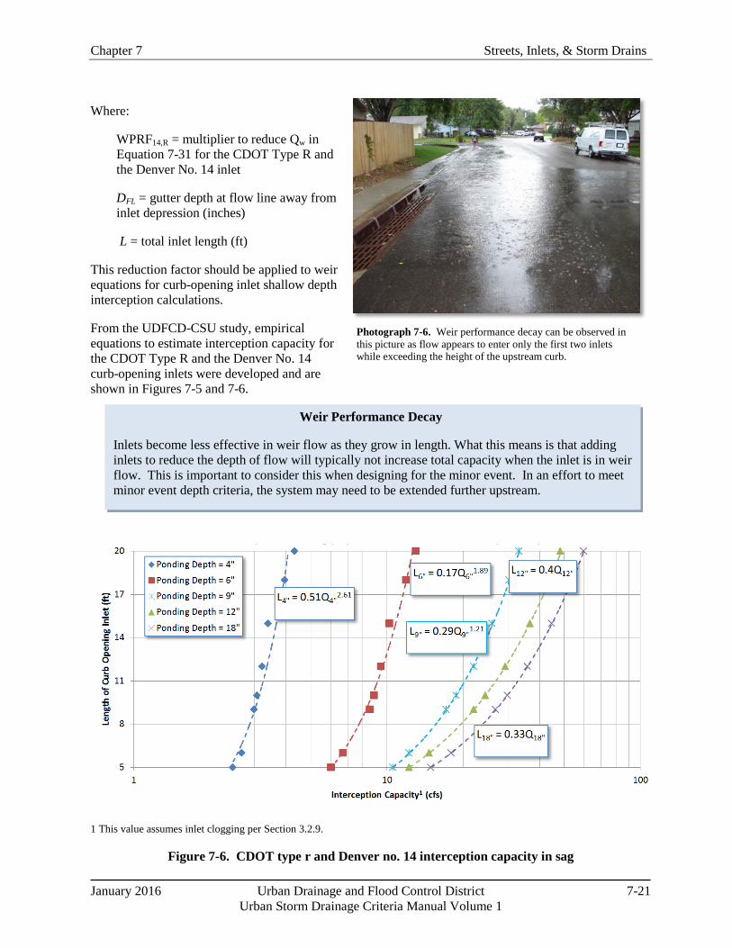
Photograph 7-6. Weir performance decay can be observed in this picture as flow appears to enter only the first two inlets while exceeding the height of the upstream curb.
Weir Performance Decay
Inlets become less effective in weir flow as they grow in length. What this means is that adding inlets to reduce the depth of flow will typically not increase total capacity when the inlet is in weir flow. This is important to consider this when designing for the minor event. In an effort to meet minor event depth criteria, the system may need to be extended further upstream.
Where:
WPRF14,R = multiplier to reduce Qw in Equation 7-31 for the CDOT Type R and the Denver No. 14 inlet
DFL = gutter depth at flow line away from inlet depression (inches)
L = total inlet length (ft)
This reduction factor should be applied to weir equations for curb-opening inlet shallow depth interception calculations.
From the UDFCD-CSU study, empirical equations to estimate interception capacity for the CDOT Type R and the Denver No. 14 curb-opening inlets were developed and are shown in Figures 7-5 and 7-6.
1 This value assumes inlet clogging per Section 3.2.9.
Figure 7-6. CDOT type r and Denver no. 14 interception capacity in sag
Streets, Inlets, & Storm Drains Chapter 7
7-22 Urban Drainage and Flood Control District January 2016 Urban Storm Drainage Criteria Manual Volume 1
For the CDOT Type 13, the Denver No. 16, and other, similar combination inlets featuring cast iron adjustable-height curb boxes, the curb-opening capacity must be added to the grate capacity as determined in Section 3.3.5. Regardless of how tall the vertical curb opening is, water captured by these curb openings must enter through a narrow horizontal opening under the curb head and in the plane of the grate. Therefore the capacity of the curb opening associated with these combination inlets is estimated based on that horizontal throat opening geometry using Equation 7-31 for the weir condition, and for the orifice condition as:
gDLWNCQ ecooo 2).0(= Equation 7-34
Where:
Wc = horizontal orifice width (typically 0.44 feet for the CDOT Type 13, the Denver No. 16, and other, similar combination inlets featuring cast iron adjustable-height curb boxes)
Once weir and orifice interception rates are calculated, Equations 7-29 and 7-30 must also be applied to the curb-opening portion of combination inlets in sag locations.
After the controlling interception rate for the grate and for the curb opening have been calculated as the minimum of the weir, orifice, and mixed flows, a reduction factor tied to the geometric mean of the grate and curb-opening capacities should be applied to the algebraic sum of the total interception as:
cgcgt QQKQQQ −+= Equation 7-35
Where:
Qt = interception capacity for combination inlet (cfs)
Qg = interception for grate (cfs)
Qc = interception for curb opening (cfs)
K = dimensionless reduction factor (= 0.37 for CDOT Type 13 combination inlet, = 0.21 for Denver No. 16 combination inlet).
A higher reduction factor implies higher interference between the grate and the curb opening. The HEC-22 procedure assumes that the grate and curb opening function independently, resulting in a consistent overestimation of the capacity of combination inlets. K is a lumped, average parameter representing the range of observed water depths in the laboratory. During the model tests, it was observed that when the grate surface area is subject to shallow water, the curb opening intercepted the flow only at its two corners, and did not behave as a side weir by collecting flow along its full length. Under deep water, vortex circulation dominates the flow pattern. As a result, the central portion of the curb opening more actively draws water into the inlet box. Equation 7-35 best represents the range of the observed data.
The UDFCD-CSU study demonstrated that the Denver No. 16 and the CDOT Type 13 combination inlets are also subject to weir performance decay, which was described above with regard to the CDOT Type R and Denver No. 14 curb-opening inlets. For the Denver No. 16 and the CDOT Type 13 combination inlets, the WPRF multiplier is found by:
Chapter 7 Streets, Inlets, & Storm Drains
January 2016 Urban Drainage and Flood Control District 7-23 Urban Storm Drainage Criteria Manual Volume 1
( )
+
=3.4,9Min7.0
,1MinWPRF 16,13 LDFL Equation 7-36
Where:
WPRF13,16 = multiplier to reduce Qw in Equation 7-31 for the CDOT Type 13 and the Denver No. 16 inlet
DFL = gutter depth at flow line away from inlet depression (inches)
L = total inlet length (ft).
This reduction factor should be applied to both the grate and the curb opening weir equations (Equation 7-31) for combination inlet shallow depth interception calculations.
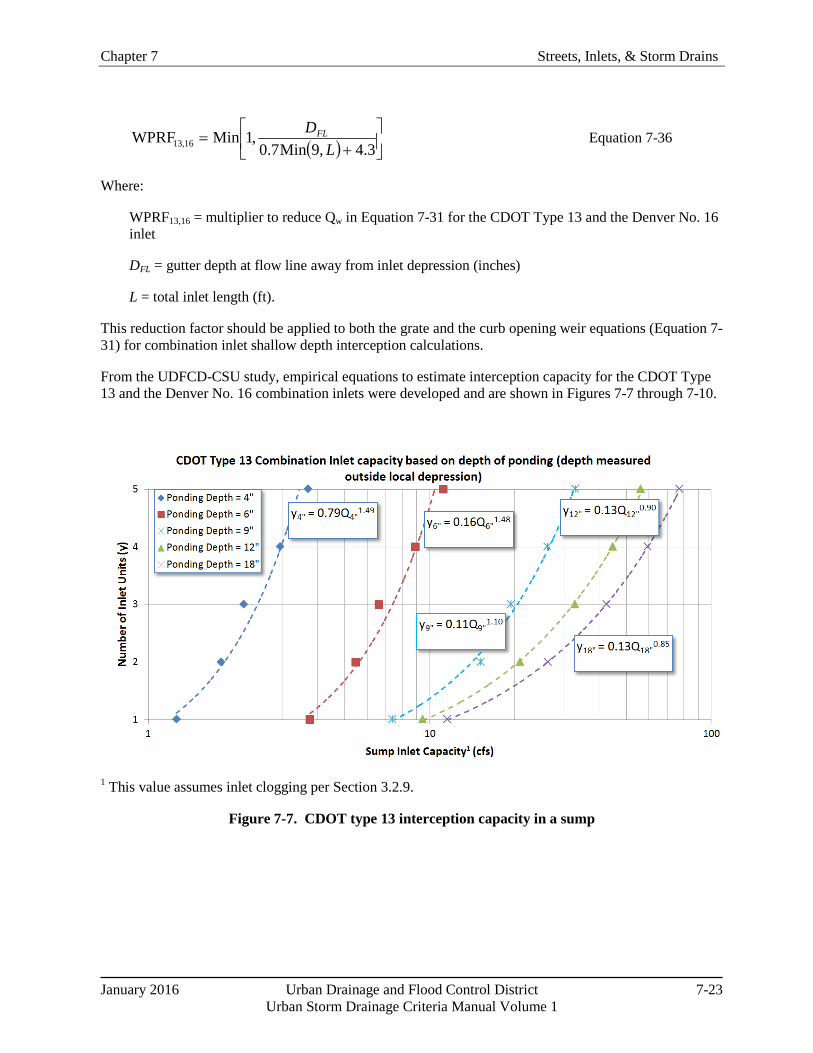
From the UDFCD-CSU study, empirical equations to estimate interception capacity for the CDOT Type 13 and the Denver No. 16 combination inlets were developed and are shown in Figures 7-7 through 7-10.
1 This value assumes inlet clogging per Section 3.2.9.
Figure 7-7. CDOT type 13 interception capacity in a sump
Streets, Inlets, & Storm Drains Chapter 7
7-24 Urban Drainage and Flood Control District January 2016 Urban Storm Drainage Criteria Manual Volume 1
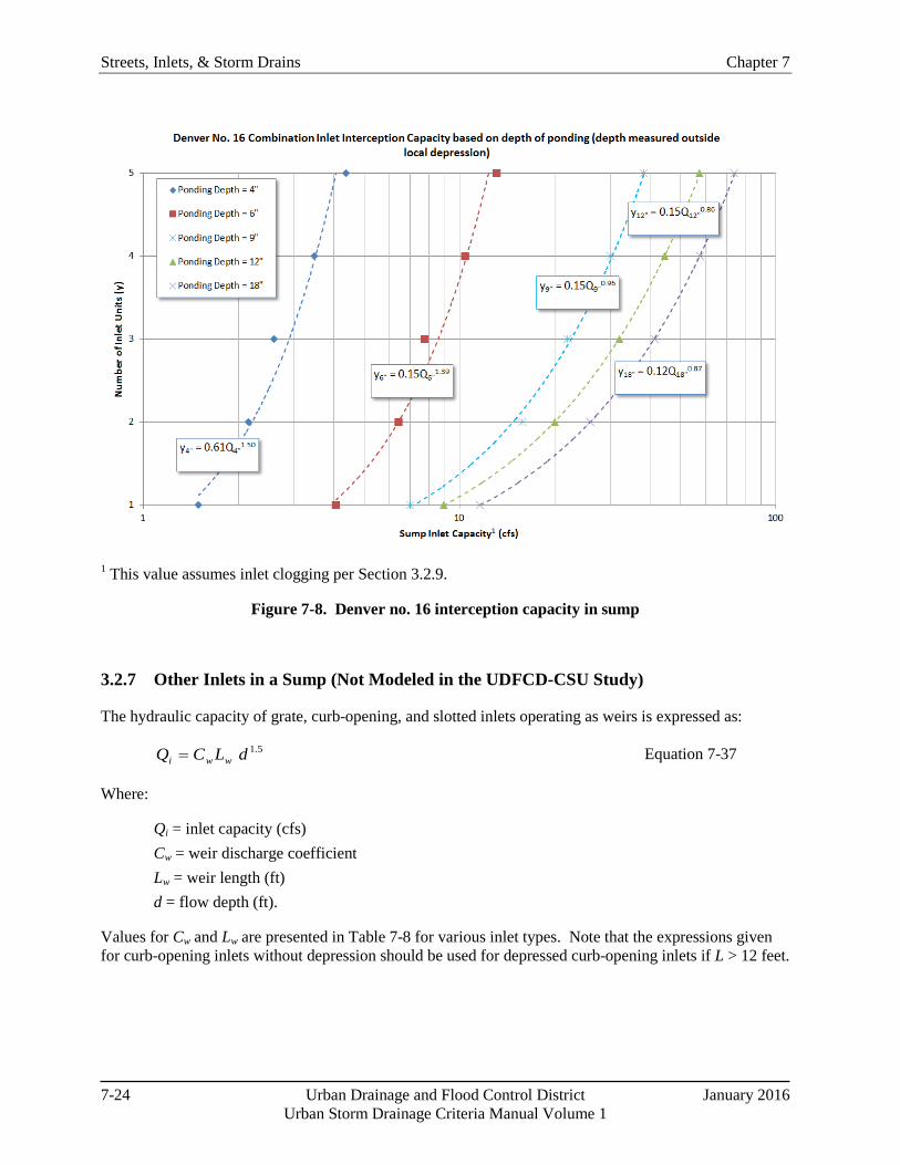
1 This value assumes inlet clogging per Section 3.2.9.
Figure 7-8. Denver no. 16 interception capacity in sump
3.2.7 Other Inlets in a Sump (Not Modeled in the UDFCD-CSU Study)
The hydraulic capacity of grate, curb-opening, and slotted inlets operating as weirs is expressed as:
5.1dLCQ wwi = Equation 7-37
Where:
Qi = inlet capacity (cfs) Cw = weir discharge coefficient Lw = weir length (ft) d = flow depth (ft).
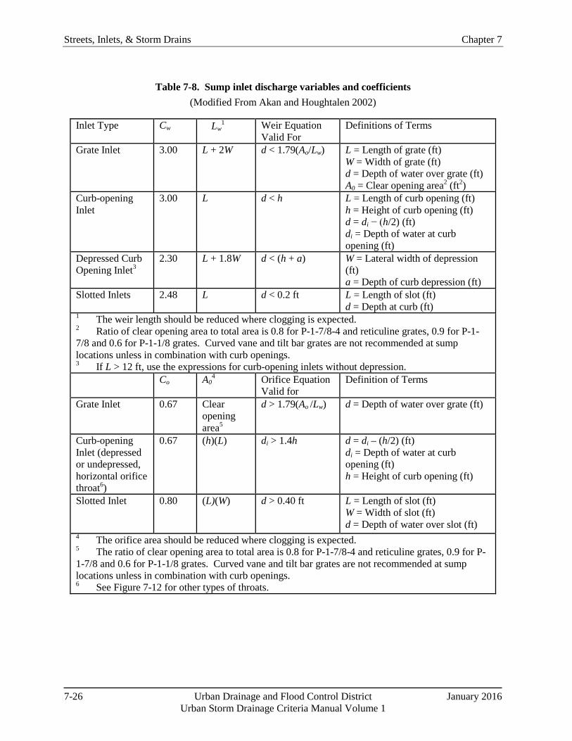
Values for Cw and Lw are presented in Table 7-8 for various inlet types. Note that the expressions given for curb-opening inlets without depression should be used for depressed curb-opening inlets if L > 12 feet.
Chapter 7 Streets, Inlets, & Storm Drains
January 2016 Urban Drainage and Flood Control District 7-25 Urban Storm Drainage Criteria Manual Volume 1
The hydraulic capacity of grate, curb-opening, and slotted inlets operating as orifices is expressed as:
( ) 5.02gdACQ ooi = Equation 7-38
Where:
Qi = inlet capacity (cfs) Co = orifice discharge coefficient Ao = orifice area (ft2) d = characteristic depth (ft) as defined in Table 7-8 g = 32.2 ft/sec2.
Values for Co and Ao are presented in Table 7-8 for different types of inlets.
Combination inlets are commonly used in sumps. The hydraulic capacity of combination inlets in sumps depends on the type of flow and the relative lengths of the curb opening and grate. For weir flow, the capacity of a combination inlet (grate length equal to the curb opening length) is equal to the capacity of the grate portion only. This is because the curb opening does not add any effective length to the weir. If the curb opening is longer than the grate, the capacity of the additional curb length should be added to the grate capacity. For orifice flow, the capacity of the curb opening should be added to the capacity of the grate.
Streets, Inlets, & Storm Drains Chapter 7
7-26 Urban Drainage and Flood Control District January 2016 Urban Storm Drainage Criteria Manual Volume 1
Table 7-8. Sump inlet discharge variables and coefficients (Modified From Akan and Houghtalen 2002)
Inlet Type Cw Lw1 Weir Equation
Valid For Definitions of Terms
Grate Inlet 3.00 L + 2W d < 1.79(Ao/Lw) L = Length of grate (ft) W = Width of grate (ft) d = Depth of water over grate (ft) A0 = Clear opening area2 (ft2)
Curb-opening Inlet
3.00 L d < h L = Length of curb opening (ft) h = Height of curb opening (ft) d = di − (h/2) (ft) di = Depth of water at curb opening (ft)
Depressed Curb Opening Inlet3
2.30 L + 1.8W d < (h + a) W = Lateral width of depression (ft) a = Depth of curb depression (ft)
Slotted Inlets 2.48 L d < 0.2 ft L = Length of slot (ft) d = Depth at curb (ft)
1 The weir length should be reduced where clogging is expected. 2 Ratio of clear opening area to total area is 0.8 for P-1-7/8-4 and reticuline grates, 0.9 for P-1-7/8 and 0.6 for P-1-1/8 grates. Curved vane and tilt bar grates are not recommended at sump locations unless in combination with curb openings. 3 If L > 12 ft, use the expressions for curb-opening inlets without depression. Co A0
4 Orifice Equation Valid for
Definition of Terms
Grate Inlet 0.67 Clear opening area5
d > 1.79(Ao /Lw) d = Depth of water over grate (ft)
Curb-opening Inlet (depressed or undepressed, horizontal orifice throat6)
0.67 (h)(L) di > 1.4h d = di – (h/2) (ft) di = Depth of water at curb opening (ft) h = Height of curb opening (ft)
Slotted Inlet 0.80 (L)(W) d > 0.40 ft L = Length of slot (ft) W = Width of slot (ft) d = Depth of water over slot (ft)
4 The orifice area should be reduced where clogging is expected. 5 The ratio of clear opening area to total area is 0.8 for P-1-7/8-4 and reticuline grates, 0.9 for P-1-7/8 and 0.6 for P-1-1/8 grates. Curved vane and tilt bar grates are not recommended at sump locations unless in combination with curb openings. 6 See Figure 7-12 for other types of throats.

Chapter 7 Streets, Inlets, & Storm Drains
January 2016 Urban Drainage and Flood Control District 7-27 Urban Storm Drainage Criteria Manual Volume 1
Figure 7-9. Perspective views of grate and curb-opening inlets
Figure 7-10. Orifice calculation depths for curb-opening inlets
(note that the equation for the inclined throat is also valid for the other cases)
Streets, Inlets, & Storm Drains Chapter 7
7-28 Urban Drainage and Flood Control District January 2016 Urban Storm Drainage Criteria Manual Volume 1
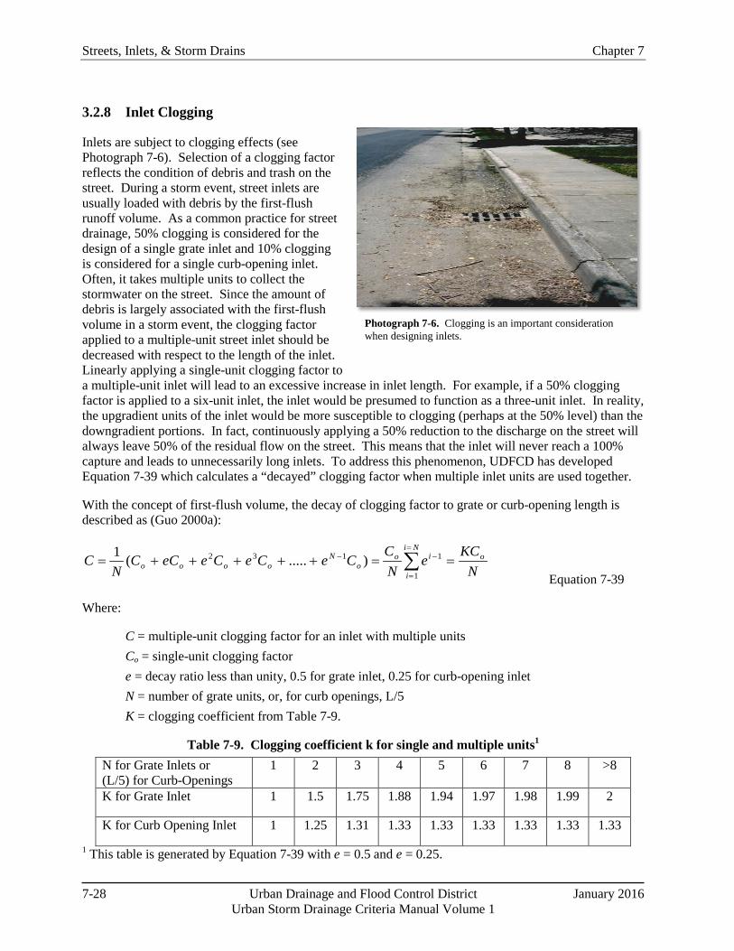
Photograph 7-6. Clogging is an important consideration when designing inlets.
3.2.8 Inlet Clogging
Inlets are subject to clogging effects (see Photograph 7-6). Selection of a clogging factor reflects the condition of debris and trash on the street. During a storm event, street inlets are usually loaded with debris by the first-flush runoff volume. As a common practice for street drainage, 50% clogging is considered for the design of a single grate inlet and 10% clogging is considered for a single curb-opening inlet. Often, it takes multiple units to collect the stormwater on the street. Since the amount of debris is largely associated with the first-flush volume in a storm event, the clogging factor applied to a multiple-unit street inlet should be decreased with respect to the length of the inlet. Linearly applying a single-unit clogging factor to a multiple-unit inlet will lead to an excessive increase in inlet length. For example, if a 50% clogging factor is applied to a six-unit inlet, the inlet would be presumed to function as a three-unit inlet. In reality, the upgradient units of the inlet would be more susceptible to clogging (perhaps at the 50% level) than the downgradient portions. In fact, continuously applying a 50% reduction to the discharge on the street will always leave 50% of the residual flow on the street. This means that the inlet will never reach a 100% capture and leads to unnecessarily long inlets. To address this phenomenon, UDFCD has developed Equation 7-39 which calculates a “decayed” clogging factor when multiple inlet units are used together.
With the concept of first-flush volume, the decay of clogging factor to grate or curb-opening length is described as (Guo 2000a):
∑=
=
−− ==+++++=Ni
i
oioo
Noooo N
KCe
NC
CeCeCeeCCN
C1
1132 ).....(1
Equation 7-39
Where:
C = multiple-unit clogging factor for an inlet with multiple units Co = single-unit clogging factor e = decay ratio less than unity, 0.5 for grate inlet, 0.25 for curb-opening inlet N = number of grate units, or, for curb openings, L/5 K = clogging coefficient from Table 7-9.
Table 7-9. Clogging coefficient k for single and multiple units1
N for Grate Inlets or (L/5) for Curb-Openings
1 2 3 4 5 6 7 8 >8
K for Grate Inlet 1 1.5 1.75 1.88 1.94 1.97 1.98 1.99 2
K for Curb Opening Inlet 1 1.25 1.31 1.33 1.33 1.33 1.33 1.33 1.33
1 This table is generated by Equation 7-39 with e = 0.5 and e = 0.25.
Chapter 7 Streets, Inlets, & Storm Drains
January 2016 Urban Drainage and Flood Control District 7-29 Urban Storm Drainage Criteria Manual Volume 1
When N becomes large, Equation 7-39 converges to:
)1( eNCC o
−= Equation 7-40
For instance, when e = 0.5 and Co = 50%, C = 1.0/N for a large number of units, N. In other words, only the first unit out of N units will be clogged. Equation 7-40 complies with the recommended clogging factor for a single-unit inlet and decays on the clogging effect for a multiple-unit inlet.
The interception of an inlet on a grade is proportional to the inlet length and, in a sump, is proportional to the inlet opening area. Therefore, a clogging factor should be applied to the length of the inlet on a grade as:
LCLe )1( −= Equation 7-41
in which Le = effective (unclogged) length (ft). Similarly, a clogging factor should be applied to the opening area of an inlet in a sump as:
ACAe )1( −= Equation 7-42
Where:
Ae = effective opening area (ft2)
A = opening area (ft2).
3.2.9 Nuisance Flows
The location of inlets is important to address the effects of nuisance flows and avoid icing. Nuisance flows are urban runoff flows that are typically most notable during dry weather and come from sources such as over-irrigation and snow melt. Nuisance flows cause problems in both warm and cold weather months. Problems include algae growth and ice. While it is possible to minimize nuisance conditions through design, irrigation practices in the summer and snow and ice removal in the winter make it very difficult to eliminate nuisance flows entirely. Because these practices are largely controlled by residents and business, municipalities should plan for maintenance to address nuisance flow conditions, particularly in the winter when ice accumulation can impede the ability of the drainage system to serve its purpose.
In the summer months, over-irrigation of lawns and landscaping can be a major contributor to nuisance flows. Car washing is another summertime cause of excess flows. In homes with poor or improper drainage, excessive sump pump discharge may also contribute.
In winter months, snow and ice melt are the primary causes of nuisance flows and associated icing problems (see Photograph 7-7). Discharges from sump pumps to the sidewalk and/or street can also lead to icing.

Streets, Inlets, & Storm Drains Chapter 7
7-30 Urban Drainage and Flood Control District January 2016 Urban Storm Drainage Criteria Manual Volume 1
Photograph 7-7. The location of inlets is important to address the effects of nuisance flows.
Flows over sidewalks and driveways due to summertime nuisance flows can cause algae growth, especially if fertilizer is being used in conjunction with over-irrigation. Such algae growth is both a safety issue due to increased falling risk resulting from slippery surfaces and an aesthetic issue. Nuisance flows laden with fertilizer, sediment, and other pollutants also have the potential to overload stormwater BMPs, which are generally designed for lower pollutant concentrations found in typical wet weather flows. Additionally, continually moist conditions can create an environment where fecal bacteria thrive, either becoming an on-going dry weather source of bacteria loading or a source that is subsequently mobilized under wet weather conditions, such as in the case of biofilm soughing.
Public education about proper irrigation rates and irrigation system maintenance (e.g., broken or misaligned sprinkler heads) can help reduce occurrences of excess flow over sidewalks. Additionally, homeowners can be encouraged to direct downspout and sump pump discharges to swales, lawns, and gardens (keeping away from foundation backfill zones) where water can infiltrate. Algae growth is encouraged by the presence of nutrients which can come from fertilizer and organic matter. Algae growth can be reduced by educating homeowners on proper application of fertilizer (both rates and timing of application), using phosphorus-free fertilizer, and sweeping up dead leaves and plant matter on impervious surfaces. Whenever feasible, impervious surfaces should be swept rather than sprayed down with water. When power-washing of outdoor surfaces is conducted, comply with local, state and federal regulations.
Snow and ice melt can re-freeze on streets and sidewalks, where it poses hazards to the public and is difficult to remove. Often, icing is most significant on east-west streets that have less solar exposure in the winter. Trees, buildings, fences and topography can also create shady areas where ice accumulates. Snow and ice may also clog drains and inlets, leading to flooding. Snowmelt has been found to have high pollutant concentrations which can stress treatment facilities. Because many of the issues related to winter nuisance flows are beyond the control of municipalities (especially in areas that are already developed), identifying problem areas and planning for maintenance is often the most effective practice for minimizing nuisance conditions.
Table 7-10 provides the various sources, problems, and avoidance strategies associated with nuisance flows.

Chapter 7 Streets, Inlets, & Storm Drains
January 2016 Urban Drainage and Flood Control District 7-31 Urban Storm Drainage Criteria Manual Volume 1
Table 7-10. Nuisance flows: sources, problems and avoidance strategies
Warm Weather Cold Weather
Examples/Sources
Over-irrigation of lawns and landscaping Snowmelt
Car washing Ice Melt
Sump pump discharge Sump pump discharge (freezing)
Problems
Poor water quality Icing leading to inlet blockage and flooding
High nutrient concentration Ice on streets and sidewalks
High pollutant concentration High pollutant concentrations
Algae Growth
Avoidance
Strategies
Irrigation, drainage, and fertilizer education
Inlet and sidewalk maintenance
Proper drainage design Prompt and frequent snow and ice removal
Minimization of directly connected impervious area
Consider additional inlets in strategic locations
Sidewalk chase drains Shoveling snow onto grassy areas away from streets and inlets
Locate inlets and sumps away from shaded areas
Homeowners, business owners, maintenance and city workers should be educated and encouraged to use proper snow and ice removal techniques. These include removal of snow and ice promptly and frequently, keeping drains and gutters clear, and placing shoveled snow onto lawns or grassy areas.

Streets, Inlets, & Storm Drains Chapter 7
7-32 Urban Drainage and Flood Control District January 2016 Urban Storm Drainage Criteria Manual Volume 1
Photograph 7-8. Inlets frequently need maintenance.
For new development projects, locating inlets in areas where water can be intercepted before it accumulates or slows down and has the opportunity to freeze is the most effective way to minimize icing from the design perspective. To the extent practical, locate inlets away from areas that will be heavily shaded during winter months (in particular the north side of buildings) to help prevent ice build-up and allow proper flow. For areas where shading is unavoidable, consider providing additional inlet capacity at strategic locations. For example, if a street with a southern exposure will drain to an east-west street that is shaded, having additional inlet capacity at the intersection may be advisable, especially if the flow is intended to turn and follow the east-west street. It is also important to consider potential future vegetative growth when evaluating shading effects. Although trees may be small and have little canopy when originally planted, they will grow and ultimately provide far greater tree canopy far greater than when initially planted. Tree canopy may vary seasonally, depending on the tree species (e.g., deciduous trees lose their leaves in the fall, so less canopy is present in the winter). Ultimately, even with careful placement of inlets and avoidance of shading to the extent practical, icing in some locations will still likely occur due to shading from buildings, fences and other improvements on private property, and maintenance to remove accumulated ice will be necessary. For areas that are already developed, maintenance (i.e., snow and ice removal) to control icing from nuisance flows is the primary method to address icing, and for many municipalities, this is an ongoing part of their street maintenance programs.
During all times of the year, it is important that nuisance flows can be properly conveyed to storm drain outlets. Ponding on streets and sidewalks promotes both ice and algae growth. Sidewalk chase drains may be appropriate to aid in proper drainage of nuisance flows (for sump pump discharges, in particular); however, sidewalk chases can be problematic in terms of clogging and icing if they are located in areas with heavy loads of gross solids (leaves, grocery bags, restaurant litter, etc.) or if they are located in areas with poor solar exposure in winter months.
For more information on nuisance flows, multiple Colorado-based publications are available to provide guidance related to landscape management practices and snow and ice removal. Representative resources include:
USDCM Volume 3, Source Control BMPs GreenCO BMP Manual Colorado State University Extension Yard and Garden Fact Sheets.
3.3 Inlet Location and Spacing on Continuous Grades
Although one should always perform interception capacity computations on stormwater inlets, the ultimate location (or positioning) of those inlets is rarely a function of interception alone. Often, inlets are required in certain locations based upon street design considerations, topography (sumps), and local ordinances. One notable exception is the location and spacing of inlets on continuous grades. On a long continuous grade, stormwater flow increases as it moves down the gutter and picks up more drainage area. As the flow increases, so does the spread and depth. Since the spread (encroachment) and depth (inundation) are not allowed to exceed some specified maximum, inlets must be strategically placed to

Chapter 7 Streets, Inlets, & Storm Drains
January 2016 Urban Drainage and Flood Control District 7-33 Urban Storm Drainage Criteria Manual Volume 1
remove some of the stormwater from the street. Locating these inlets requires design computations by the engineer.
3.3.1 Design Considerations
The primary design considerations for the location and spacing of inlets on continuous grades are the encroachment and inundation limitations. This was addressed in Section 2.2. Table 7-2 lists pavement encroachment and inundation standards for minor storms in the UDFCD region.
Proper design of stormwater collection and conveyance systems makes optimum use of the conveyance capabilities of street gutters, such that an inlet is not needed until the spread (encroachment) and depth (inundation) reach allowable limits during the design (minor) storm. To place an inlet prior to that point on the street is not economically efficient. To place an inlet after that point would violate the encroachment and inundation standards. Therefore, the primary design objective is to position inlets along a continuous grade at the locations where the allowable spread and/or depth is about to be exceeded for the design storm.
3.3.2 Design Procedure
Based on the encroachment and inundation standards and the given street geometry, the allowable street hydraulic capacity can be determined using Equation 7-11 and Equation 7-12. This flow rate is then equated to some hydrologic technique (equation) that contains drainage area. In this way, the inlet is positioned on the street so that it will service the requisite drainage area. The process of locating the inlet is accomplished by trial-and-error. If the inlet is moved downstream (or down gutter), the drainage area increases. If the inlet is moved upstream, the drainage area decreases.
The hydrologic technique most often used in urban drainage design is the rational method. The rational method was discussed in the Runoff chapter. The rational method, repeated here for convenience, is:
CIAQ = Equation 7-43
Where:
Q = peak discharge (cfs) C = runoff coefficient described in the Runoff chapter I = design storm rainfall intensity (in/hr) described in the Rainfall chapter A = drainage area (acres).
The design process starts with the selection of the proposed first inlet in the system. The peak discharge for the half-street at this point is calculated by the rational method, using runoff coefficients and rainfall intensities as described in the Runoff Chapter. Next, the allowable peak discharge is found using the allowable spread and depth calculated as functions of the street geometry at the design point. If the allowable peak discharge is less than the watershed peak discharge, the proposed design point is too far downstream in the watershed and must be moved upstream. If the allowable peak discharge is much greater than the calculated peak discharge, no inlet is required at the proposed design point and a new location for the proposed first inlet in the system is selected somewhere downstream of this location. The ultimate goal is to always place an inlet just upstream of the point where the allowable spread and/or depth criteria would otherwise be exceeded.
Once the first inlet location is identified along a continuous grade, an inlet type and size can be specified. The first inlet’s hydraulic capacity is then assessed. Generally, it is uneconomical to size an inlet (on

Streets, Inlets, & Storm Drains Chapter 7
7-34 Urban Drainage and Flood Control District January 2016 Urban Storm Drainage Criteria Manual Volume 1
continuous grades) large enough to capture all of the gutter flow. Instead, some carryover flow is expected. This practice reduces the amount of new flow that can be picked up at the next inlet. However, each inlet should be positioned at the location where the spread or depth of flow is about to reach its allowable limit.
The gutter discharge for inlets (other than the most upstream inlet), consists of the carryover (bypassed) flow from the upstream inlet plus the stormwater runoff generated from the intervening local drainage area. The carryover flow from the upstream inlet is added to the peak flow rate obtained from the rational method for the intervening local drainage area. The resulting peak flow is conservatively approximate since the carryover flow peak and the local runoff peak do not necessarily coincide.
4.0 Storm Drain Systems
4.1 Introduction
Once stormwater is collected from the street by an inlet, it is directed into the storm drain system. The storm drain system is comprised of inlets, pipes, manholes, bends, outlets, and other appurtenances. For specific information regarding the applicability of a number of available pipe materials, a document titled “Storm Sewer Pipe Material Technical Memorandum” is available for download at www.udfcd.org.
Apart from inlets, manholes are the most common appurtenance in storm drain systems. Their primary functions include:
Providing maintenance access.
Serving as junctions when two or more pipes merge.
Providing flow transitions for changes in pipe size, slope, and alignment.
Providing ventilation.
Manholes are generally made of pre-cast or cast-in-place reinforced concrete. They are typically four to five feet in diameter and are required at regular intervals, even in straight sections, for maintenance reasons. Standard size manholes cannot accommodate large pipes, so special junction vaults are constructed for that application.
Occasionally, bends and transitions are accomplished without manholes, particularly for large pipe sizes. These sections provide gradual transitions in size or alignment to minimize energy losses. Outlet structures, covered in the Hydraulic Structures chapter, are transitions from pipe flow into open channel flow or still water (e.g., ponds, lakes, etc.). Their primary function is to provide a transition that minimizes erosion in the receiving water body. Occasionally, flap gates or other types of check valves are placed on outlet structures to prevent backflow from high tailwater or flood-prone receiving waters.
4.2 Design Process, Considerations, and Constraints
The design of a storm drain system requires a large data collection effort. The data requirements in the proposed service area include topography, drainage boundaries, imperviousness, soil types, and locations of any existing storm drain conduits, inlets, and manholes. In addition, identification of the type and location of other utilities in the ground is critical. Alternative layouts of a new system (or modifications to an existing system) can be investigated using these data.
System layouts rely largely on street rights-of-way and topography. Most layouts are dendritic (tree)
Chapter 7 Streets, Inlets, & Storm Drains
January 2016 Urban Drainage and Flood Control District 7-35 Urban Storm Drainage Criteria Manual Volume 1
networks that follow the street pattern. Dendritic networks collect stormwater from a broad area and converge in the downstream direction. Networks with parallel branches are possible but are less common and require full hydraulic modeling. Each layout should depict inlet and manhole locations, drainage boundaries serviced by the inlets, pipe locations, flow directions, and outlet locations. A final layout selection is made from the viable alternatives based on likely system performance and cost.
Once a final layout is chosen, storm drain pipes are sized based on the hydrology (peak flows) and hydraulics (pipe capacities). This is accomplished by designing the upstream pipes first and moving downstream. Pipe diameters less than 15 inches are not recommended for storm drains, and many communities have adopted an 18-inch diameter minimum standard. Pipes generally increase in size moving downstream since the drainage area (and thus flow) is increasing. Downstream pipes should never be smaller than upstream pipes, even if a steeper slope is encountered that will provide sufficient capacity with a smaller pipe. The potential for clogging at the resulting “choke point” is always a concern.
Storm drains are typically sized to convey the minor storm without surcharging, using open channel hydraulics calculations to determine normal depth 100% full pipe depth. Because the maximum capacity of a circular pipe occurs at approximately 93% of the depth of full pipe flow, designing for full flow will result in slightly conservative design. The minor storm typically is defined by a return interval from the 2-year to the 5-year storm depending on the function of the infrastructure being served. Refer to the Policy chapter for guidance regarding selection of the design storm.
Manholes are located in the system in conjunction with pipe sizing and inlet placement, where manhole locations are dictated by standard design practices. For example, manholes are required whenever there is a lateral pipe servicing an inlet, and where a change occurs in pipe size, alignment, or slope. In addition, manholes are required at pipe branch junctions. Manholes are also required along long straight sections of pipe for maintenance purposes, with the distance between manholes dependent on pipe size, but not more than 400 feet. The invert of a pipe leaving a manhole should be at least 0.1 foot lower than the incoming pipe to ensure positive low flows through the manhole. Whenever possible, match the pipe soffit elevations when the downstream pipe is larger to minimize backwater effects on the upstream pipe. Additional manholes may be necessary to “step down” a steep grade, allowing pipe slopes to be much flatter than the slope of the street above. This is done to prevent velocities in storm drain pipes from exceeding the recommended maximum velocity of 20 ft/sec.
Once storm drain pipes are sized and manhole locations are determined, the performance of the storm drain system must be evaluated using energy grade line calculations starting at the downstream system outlet. As stormwater flows through the storm drain system, it encounters many flow transitions. These transitions include changes in pipe size, slope and alignment, as well as entrance and exit conditions. All of these transitions consume energy, resulting in energy losses expressed as head losses. These losses must be accounted for to ensure that inlets and manholes do not surcharge to a significant degree (i.e., produce street flooding). This is accomplished using hydraulic grade line (HGL) calculations as a check on pipe sizes and system losses. If significant surcharging occurs, the pipe sizes should be increased. High tailwater conditions at the storm drain outlet may also produce surcharging. This can also be accounted for using HGL calculations.
Streets, Inlets, & Storm Drains Chapter 7
7-36 Urban Drainage and Flood Control District January 2016 Urban Storm Drainage Criteria Manual Volume 1
4.3 Storm Drain Hydrology—Peak Runoff Calculation
The rational method is commonly used to determine the peak flow rates that storm drain systems must be able to convey. It is an appropriate method for the small drainage areas typically involved. It is also relatively easy to use and provides reasonable estimates of peak runoff. The total drainage area contributing flow to a particular storm drain is sometimes divided into smaller subcatchments. The rational method is described in the Runoff chapter of the USDCM.
The first pipe in a storm drain system is sized using Equation 7-43 to determine the peak flow. Downstream pipes receive flow from the upstream pipes as well as local inflows. The rational method applied to the downstream pipes is:
Equation 7-44
Where:
I = rainfall intensity based on the time of concentration for the total contributing area (in/hr) n = number of subcatchments above the stormwater pipe Cj = runoff coefficient of subcatchment j Aj = drainage area of subcatchment j (acres)
In using this equation, it is evident that the peak flow changes at each design point since the time of concentration, and thus the average intensity, changes at each design point. It is also evident that the time of concentration coming from the local inflow may differ from that coming from upstream pipes. Normally, the longest time of concentration is chosen for design purposes. If this is the case, all of the subcatchments above the design point will be included in Equation 7-44, and it usually produces the largest peak flow. On occasion, the peak flow from a shorter path may produce the greater peak discharge if the downstream areas are heavily developed. It is good practice to check all alternative flow paths and tributary areas to determine the tributary zone that produces the biggest design flow, especially when some of the tributary areas are highly impervious with rapid runoff responses.
4.4 Storm Drain Hydraulics (Gravity Flow in Circular Conduits)
4.4.1 Flow Equations and Storm Drain Sizing
Storm drain flow is unsteady and non-uniform. However, for design purposes it can be assumed to be steady and uniform at the peak flow rate, thereby allowing Manning’s equation to be applied for determining pipe capacity:
213249.1fSAR
nQ = Equation 7-45
Where:
Q = flow rate (cfs) n = Manning’s roughness factor A = flow area (ft2)
AC j
n
jj
IQ ∑=
=1
Chapter 7 Streets, Inlets, & Storm Drains
January 2016 Urban Drainage and Flood Control District 7-37 Urban Storm Drainage Criteria Manual Volume 1
R = hydraulic radius (ft) Sf = friction slope (normally assumed to be the storm drain slope) (ft/ft)
For full flow in a circular storm drain,
4
2DAA fπ
== Equation 7-46
4DRR f == Equation 7-47
Where:
D = pipe diameter (ft) Af = flow area at full flow (ft2) Rf = hydraulic radius at full flow (ft).
If the flow is pressurized (i.e., surcharging at the manholes or inlets is occurring), Sf ≠ So where So is the longitudinal slope of the storm drain pipe. Design of storm drains assumes just-full flow, a reference condition referring to steady, uniform flow with a flow depth, y, nearly equal to the pipe diameter, D. Just-full flow discharge, Qf , is calculated using:
213249.1offf SRA
nQ = Equation 7-48
Computations of flow characteristics for partial depths in circular pipes are tedious. Design aids like the UD-Culvert Excel workbook are very helpful when this is necessary.
Storm drains are sized to flow just full (i.e., as open channels using nearly the full capacity of the pipe). The design discharge is determined first using the rational method as previously discussed, then the Manning’s equation is used (with Sf = So) to determine the required pipe size. For circular pipes,
8/316.2
=
or S
nQD Equation 7-49
Where Dr is the minimum size pipe required to convey the design flow and Q is peak design flow. However, the pipe diameter that should be used in the field is the next standard pipe size larger than Dr.
The typical process proceeds as follows. Initial storm drain pipe sizing is performed first using the rational method in conjunction with Manning’s equation. The rational method is used to determine the peak discharge that storm drains must convey. The storm drain pipes are then initially sized using Manning’s equation assuming uniform, steady flow at the peak. Finally, these initial pipe sizes are checked using the energy equation by accounting for all head losses. If the energy computations detect surcharging at manholes or inlets, the pipe sizes are increased.

Streets, Inlets, & Storm Drains Chapter 7
7-38 Urban Drainage and Flood Control District January 2016 Urban Storm Drainage Criteria Manual Volume 1
4.4.2 Energy Grade Line and Head Losses
Head losses must be accounted for in the design of storm drains in order to find the energy grade line (EGL) and the hydraulic grade line (HGL) at any point in the system. The FHWA (1996) gives the following equation as the basis for calculating the head losses at inlets, manholes, and junctions (hLM, in feet):
=
gV
CCCCCKh oBpQdDoLM 2
2
Equation 7-50
Where:
Ko = initial loss coefficient Vo = velocity in the outflow pipe (ft/sec) g = gravitational acceleration (32.2 ft/sec2) CD, Cd, CQ, Cp, and CB = correction factors for pipe size, flow depth, relative flow, plunging flow and benching.
However, this equation is valid only if the water level in the receiving inlet, junction, or manhole is above the invert of the incoming pipe. Otherwise, another protocol has to be used to calculate head losses at manholes. What follows is a modified FHWA procedure that engineers can use to calculate the head losses and the EGL along any point in a storm drain system.
The EGL represents the energy slope between the two adjacent manholes in a storm drain system. A manhole may have multiple incoming storm drains, but only one outgoing drain. Each drain and its downstream and upstream manholes form a pipe-manhole unit. The entire storm drain system can be decomposed into a series of pipe-manhole units that satisfy the energy conservation principle. The computation of the EGL does this by repeating the energy-balancing process for each pipe-manhole unit.
As illustrated in Figure 7-13, a pipe-manhole unit has four distinctive sections. Section 1 is inside the downstream manhole, Section 2 is the point at the exit of the pipe just upstream of this manhole, Section 3 is just inside the upstream end of the pipe at the upstream manhole, and Section 4 is inside the upstream manhole. For each pipe-manhole unit, the head losses are determined separately in two parts as:
Friction losses through the pipe, and
Junction losses at the manhole.
The discussion that follows explains how to apply energy balancing to calculate the EGL through each pipe-manhole unit.
Losses at the Downstream Manhole, Section 1 to Section 2 The continuity of the EGL is determined between the flow conditions at centerline of the downstream manhole, Section 1, and the exit of the incoming pipe, Section 2, as illustrated in Figure 7-13 and idealized EGL and HGL profiles in Figure 7-14.
At Section 2 there may be pipe-full flow, supercritical open channel flow, critical open channel flow, or subcritical open channel flow. If the pipe soffit at the exit is submerged, the EGL at the downstream manhole provides a tailwater condition; otherwise, the manhole drop can create a discontinuity in the EGL. Therefore, it is necessary to evaluate the two possibilities, namely:
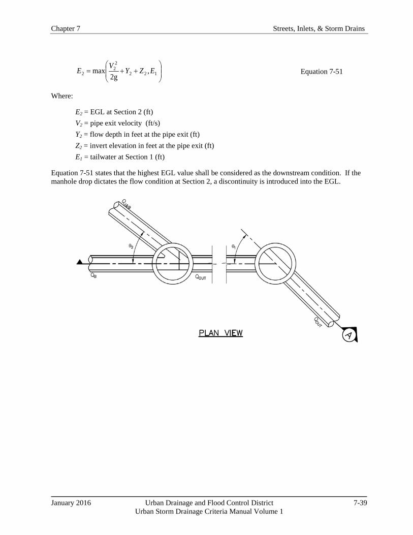
Chapter 7 Streets, Inlets, & Storm Drains
January 2016 Urban Drainage and Flood Control District 7-39 Urban Storm Drainage Criteria Manual Volume 1
++= 122
22
2 ,2g
max EZYVE Equation 7-51
Where:
E2 = EGL at Section 2 (ft) V2 = pipe exit velocity (ft/s) Y2 = flow depth in feet at the pipe exit (ft) Z2 = invert elevation in feet at the pipe exit (ft) E1 = tailwater at Section 1 (ft)
Equation 7-51 states that the highest EGL value shall be considered as the downstream condition. If the manhole drop dictates the flow condition at Section 2, a discontinuity is introduced into the EGL.

Streets, Inlets, & Storm Drains Chapter 7
7-40 Urban Drainage and Flood Control District January 2016 Urban Storm Drainage Criteria Manual Volume 1
Figure 7-11. A pipe-manhole unit
Figure 7-12. Hydraulic and energy grade lines

Chapter 7 Streets, Inlets, & Storm Drains
January 2016 Urban Drainage and Flood Control District 7-41 Urban Storm Drainage Criteria Manual Volume 1
Losses in the Pipe, Section 2 to Section 3 The continuity of the EGL within the pipe depends on the friction losses through the pipe. The flow in the pipe can be one condition or a combination of open channel flow, full flow, or pressurized (surcharge) flow. When a free surface exists through the pipe length, open channel hydraulics apply to the backwater surface profile computations. The friction losses through the pipe are the primary head losses for the type of water surface profile in the pipe. For instance, the pipe carrying a subcritical flow may have an M-1 water surface profile if the water depth at the downstream manhole is greater than normal depth in the pipe or an M-2 water surface profile if the water depth in the downstream manhole is lower than normal depth. Under an alternate condition, the pipe carrying a supercritical flow may have an S-2 water surface profile if the pipe entering the downstream manhole is not submerged; otherwise, a hydraulic jump is possible within the pipe.
When the downstream pipe soffit is submerged to a degree that the entire pipe is under the HGL, the head loss for this full flow condition is estimated by pressure flow hydraulics.
When the downstream pipe soffit is slightly submerged, the downstream end of the pipe is surcharged, but the upstream end of the pipe can have open channel flow. The head loss through a surcharge flow depends on the flow regime. For a subcritical flow, the head loss is the sum of the friction losses for the full flow condition and for the open channel flow condition. For a supercritical flow, the head loss may involve a hydraulic jump. To resolve which condition governs, culvert hydraulic principles can be used under both inlet and outlet control conditions and the governing condition is the one that produces the highest HGL at the upstream manhole.
Having identified the type of flow in the pipe, the computation of friction losses begins with the determination of friction slope. The friction loss and energy balance are calculated as:
ff LSh = Equation 7-52
∑+= fhEE 23 Equation 7-53
Where:
hf = friction loss (ft) L = length of pipe (ft) Sf = friction slope in the pipe (ft/ft) E3 = EGL at the upstream end of pipe (ft)
Losses at the Upstream Manhole, Section 3 to Section 4
Additional losses may be introduced at the pipe entrance. The general formula to estimate the entrance loss is:
gVKh EE 2
2
= Equation 7-54
Where:
hE = entrance loss (ft) V = pipe-full velocity in the incoming pipe (ft/s)
Streets, Inlets, & Storm Drains Chapter 7
7-42 Urban Drainage and Flood Control District January 2016 Urban Storm Drainage Criteria Manual Volume 1
KE = entrance loss coefficient between 0.2 to 0.5
In the modeling of pipe flow, the pipe entrance coefficients can be assumed to be part of the bend loss coefficient.
The energy principle between Sections 3 and 4 is determined by:
EhEE += 34 Equation 7-55
Where:
E4 = EGL at Section 4 (ft)
Junction and Bend Losses at the Upstream Manhole, Section 4 to Section 1 The analysis from Section 4 of the downstream pipe-manhole unit to Section 1 of the upstream pipe-manhole unit consists only of junction losses through the manhole. To maintain the conservation of energy through the manhole, the outgoing energy plus the energy losses at the manhole have to equal the incoming energy. Often a manhole is installed for the purpose of maintenance, deflection of the pipe alignment, change of the pipe size, and as a junction for incoming laterals. Although there are different causes for junction losses, they are typically considered as a minor loss in the computation of the EGL. These junction losses in the pipe system are determined solely by the local configuration and geometry and not by the length of the flow path through the manhole. Bend/Deflection Losses The angle between the incoming pipe line and the centerline of the exiting main pipe line introduces a bend loss to the incoming pipe. Bend loss is estimated by:
gVKh bb 2
2
= Equation 7-56
Where:
hb = bend loss (ft) V = full flow velocity in the incoming pipe (ft/s) Kb = bend loss coefficient.
As shown in Figure 7-15 and Table 7-11, the value of Kb depends on the angle between the exiting pipe line and the existence of manhole bottom shaping. A shaped manhole bottom or a deflector guides the flow and reduces bend loss. Figure 7-16 illustrates four cross-section options for the shaping of a manhole bottom. Only sections “c. Half” and “d. Full” can be considered for the purpose of using the bend loss coefficient for the curve on Figure 7-15 labeled as “Bend at Manhole, Curved or Shaped.”
Because a manhole may have multiple incoming pipes, Equation 7-56 should be applied to each incoming pipe based on its incoming angle, and then the energy principle between Sections 4 and 1 can be calculated as:
bhEE += 41 Equation 7-57
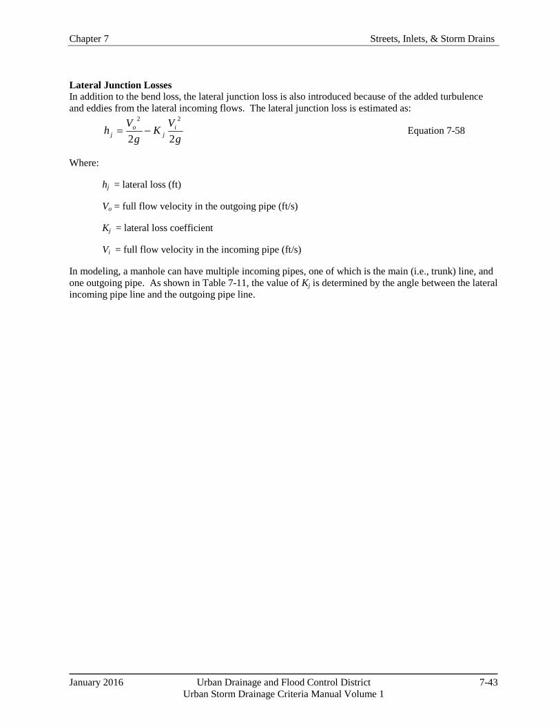
Chapter 7 Streets, Inlets, & Storm Drains
January 2016 Urban Drainage and Flood Control District 7-43 Urban Storm Drainage Criteria Manual Volume 1
Lateral Junction Losses In addition to the bend loss, the lateral junction loss is also introduced because of the added turbulence and eddies from the lateral incoming flows. The lateral junction loss is estimated as:
gV
Kg
Vh i
jo
j 22
22
−= Equation 7-58
Where:
hj = lateral loss (ft)
Vo = full flow velocity in the outgoing pipe (ft/s)
Kj = lateral loss coefficient
Vi = full flow velocity in the incoming pipe (ft/s)
In modeling, a manhole can have multiple incoming pipes, one of which is the main (i.e., trunk) line, and one outgoing pipe. As shown in Table 7-11, the value of Kj is determined by the angle between the lateral incoming pipe line and the outgoing pipe line.
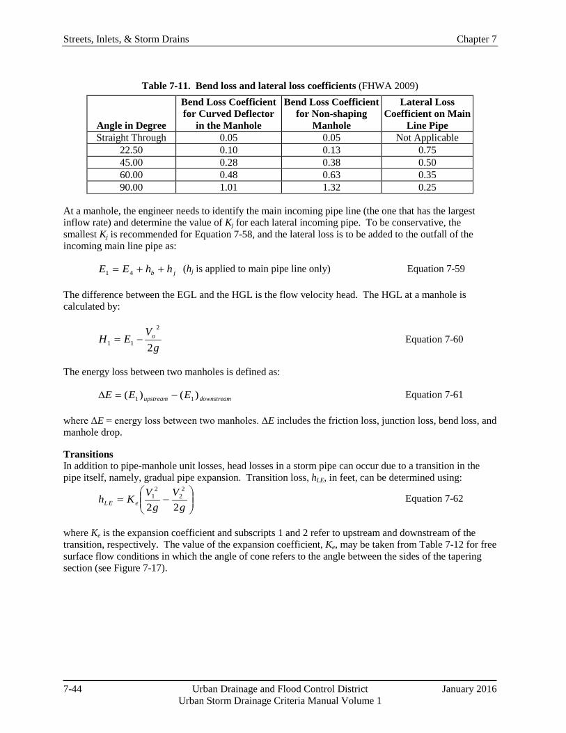
Streets, Inlets, & Storm Drains Chapter 7
7-44 Urban Drainage and Flood Control District January 2016 Urban Storm Drainage Criteria Manual Volume 1
Table 7-11. Bend loss and lateral loss coefficients (FHWA 2009)
Angle in Degree
Bend Loss Coefficient for Curved Deflector
in the Manhole
Bend Loss Coefficient for Non-shaping
Manhole
Lateral Loss Coefficient on Main
Line Pipe Straight Through 0.05 0.05 Not Applicable
22.50 0.10 0.13 0.75 45.00 0.28 0.38 0.50 60.00 0.48 0.63 0.35 90.00 1.01 1.32 0.25
At a manhole, the engineer needs to identify the main incoming pipe line (the one that has the largest inflow rate) and determine the value of Kj for each lateral incoming pipe. To be conservative, the smallest Kj is recommended for Equation 7-58, and the lateral loss is to be added to the outfall of the incoming main line pipe as:
jb hhEE ++= 41 (hj is applied to main pipe line only) Equation 7-59
The difference between the EGL and the HGL is the flow velocity head. The HGL at a manhole is calculated by:
gV
EH o
2
2
11 −= Equation 7-60
The energy loss between two manholes is defined as:
downstreamupstream EEE )()( 11 −=∆ Equation 7-61
where ΔE = energy loss between two manholes. ΔE includes the friction loss, junction loss, bend loss, and manhole drop.
Transitions In addition to pipe-manhole unit losses, head losses in a storm pipe can occur due to a transition in the pipe itself, namely, gradual pipe expansion. Transition loss, hLE, in feet, can be determined using:
−=
gV
gVKh eEL 22
22
21 Equation 7-62
where Ke is the expansion coefficient and subscripts 1 and 2 refer to upstream and downstream of the transition, respectively. The value of the expansion coefficient, Ke, may be taken from Table 7-12 for free surface flow conditions in which the angle of cone refers to the angle between the sides of the tapering section (see Figure 7-17).
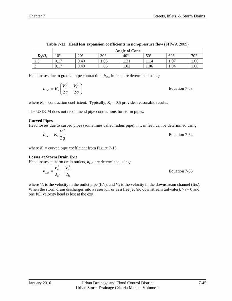
Chapter 7 Streets, Inlets, & Storm Drains
January 2016 Urban Drainage and Flood Control District 7-45 Urban Storm Drainage Criteria Manual Volume 1
Table 7-12. Head loss expansion coefficients in non-pressure flow (FHWA 2009)
D2/D1
Angle of Cone 10° 20° 30° 40° 50° 60° 70°
1.5 0.17 0.40 1.06 1.21 1.14 1.07 1.00 3 0.17 0.40 .86 1.02 1.06 1.04 1.00
Head losses due to gradual pipe contraction, hLC, in feet, are determined using:
−=
gV
gVKh cCL 22
21
22 Equation 7-63
where Kc = contraction coefficient. Typically, Kc = 0.5 provides reasonable results.
The USDCM does not recommend pipe contractions for storm pipes.
Curved Pipes Head losses due to curved pipes (sometimes called radius pipe), hLr, in feet, can be determined using:
gVKh rrL 2
2
= Equation 7-64
where Kr = curved pipe coefficient from Figure 7-15.
Losses at Storm Drain Exit Head losses at storm drain outlets, hLO, are determined using:
gV
gV
h doOL 22
22
−= Equation 7-65
where Vo is the velocity in the outlet pipe (ft/s), and Vd is the velocity in the downstream channel (ft/s). When the storm drain discharges into a reservoir or as a free jet (no downstream tailwater), Vd = 0 and one full velocity head is lost at the exit.

Streets, Inlets, & Storm Drains Chapter 7
7-46 Urban Drainage and Flood Control District January 2016 Urban Storm Drainage Criteria Manual Volume 1
D
40 60 80 900 200
0.2
0.4
0.6
0.8
1.0
1.2
Loss
Coe
fficie
nt, k
Curved Sewer r/D >6
Curved Sewer r/D = 2
Deflection Angle , in Degrees
Curved
Sewer
Bend at Manhole,Curved or Shaped
Curved or Shaped Bend at Manhole
r
Figure 7-13. Bend loss coefficients

Chapter 7 Streets, Inlets, & Storm Drains
January 2016 Urban Drainage and Flood Control District 7-47 Urban Storm Drainage Criteria Manual Volume 1
Figure 7-14. Manhole benching methods
Figure 7-15. Angle of cone for pipe diameter changes
Streets, Inlets, & Storm Drains Chapter 7
7-48 Urban Drainage and Flood Control District January 2016 Urban Storm Drainage Criteria Manual Volume 1
5.0 UD-Inlet Design Workbook The UD-Inlet design workbook provides quick solutions for many of the street capacity and inlet performance computations described in this chapter. A brief summary of each worksheet of the workbook is provided below. Note that some of the symbols and nomenclature in the worksheets do not correspond exactly with the nomenclature of the text. The text and the worksheets are computationally equivalent. An example problem using UD-Inlet is provided in section 6.0 of this chapter.
The Q-Peak tab calculates the peak discharge for the inlet tributary area based on the rational method for the minor and major storm events. Alternatively, the user can enter a known flow. Information from this tab is exported to the Inlet Management tab.
The Inlet Management tab imports information from the Q-Peak tab and Inlet [#] tabs and can be used to connect inlets in series so that bypass flow from an upstream inlet is added to flow calculated for the next downstream inlet. This tab can also be used to modify design information imported from the Q-Peak tab.
Inlet [#] tabs are created each time the user exports information from the Q-Peak tab to the Inlet Management tab. The Inlet [#] tabs calculate allowable half-street capacity based on allowable depth and allowable spread for the minor and major storm events. This is also where the user selects an inlet type and calculates the capacity of that inlet.
The Inlet Pictures tab contains a library of photographs of the various types of inlets contained in the worksheet and referenced in this chapter.
6.0 Examples
6.1 Example—Triangular Gutter Capacity
A triangular gutter has a longitudinal slope of 1%, cross slope of 2%, and a curb depth of 6 inches. Determine the flow rate and flow depth if the spread is limited to 9 feet.
Using Equation 7-1 the flow rate is calculated as:
3/82/13/556.0 TSSn
Q ox=
( )( )( )3/82/13/5 901.002.0016.056.0
=Q = 1.81 cfs
The flow depth can be found using Equation 7-2:
y = (9.0)(0.02) = 0.18 ft
Note that the computed flow depth is less than the curb height of 6 inches (0.5 feet). If it was not, the spread and associated flow rate would need to be reduced.
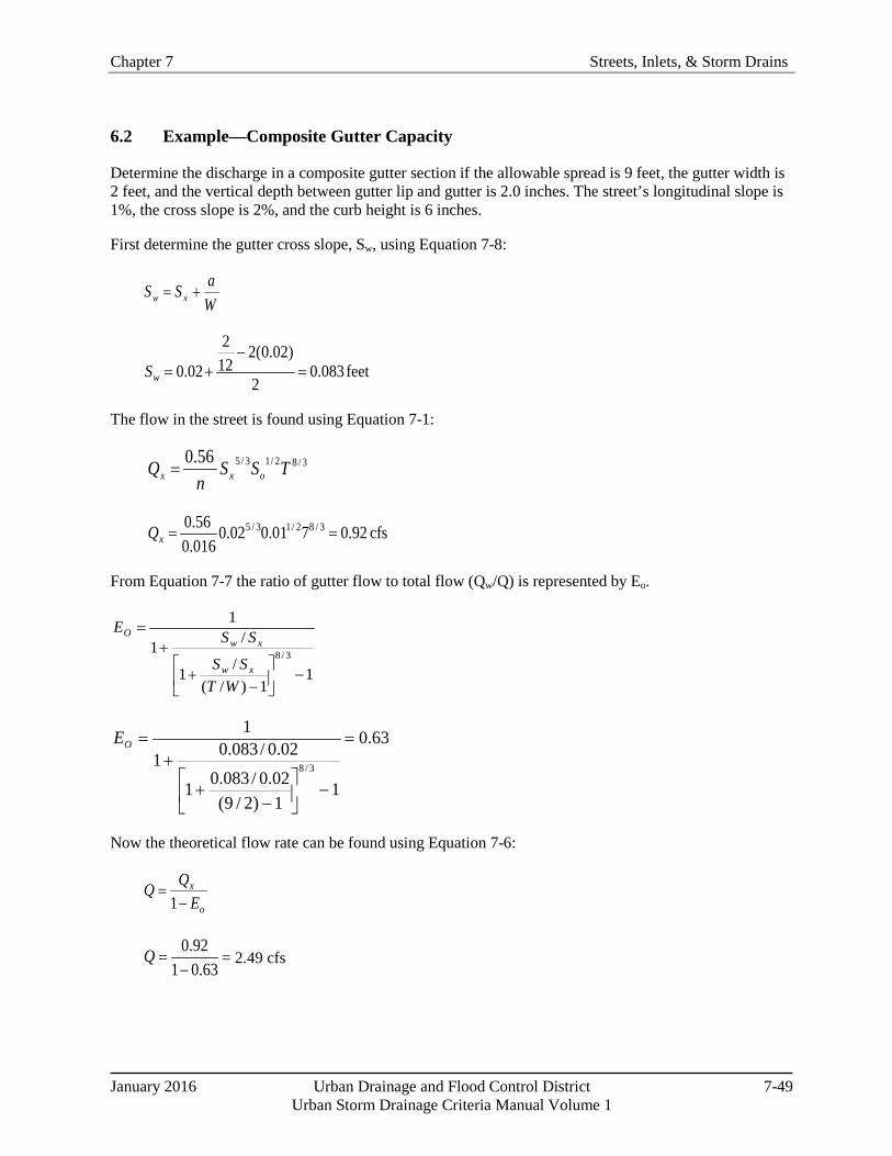
Chapter 7 Streets, Inlets, & Storm Drains
January 2016 Urban Drainage and Flood Control District 7-49 Urban Storm Drainage Criteria Manual Volume 1
6.2 Example—Composite Gutter Capacity
Determine the discharge in a composite gutter section if the allowable spread is 9 feet, the gutter width is 2 feet, and the vertical depth between gutter lip and gutter is 2.0 inches. The street’s longitudinal slope is 1%, the cross slope is 2%, and the curb height is 6 inches.
First determine the gutter cross slope, Sw, using Equation 7-8:
feet 083.02
)02.0(2122
02.0 =−
+=wS
The flow in the street is found using Equation 7-1:
3/82/13/556.0 TSSn
Q oxx =
cfs 92.0701.002.0016.056.0 3/82/13/5 ==xQ
From Equation 7-7 the ratio of gutter flow to total flow (Qw/Q) is represented by Eo.
11)/(
/1
/1
1
3/8
−
−
+
+=
WTSS
SSE
xw
xwO
0.63
11)2/9(02.0/083.01
02.0/083.01
1
3/8
=
−
−
+
+=OE
Now the theoretical flow rate can be found using Equation 7-6:
o
x
EQQ−
=1
63.0192.0
−=Q = 2.49 cfs
WaSS xw +=
Streets, Inlets, & Storm Drains Chapter 7
7-50 Urban Drainage and Flood Control District January 2016 Urban Storm Drainage Criteria Manual Volume 1
Then by using Equation 7-9 the computed flow depth is:
xTSay +=
[ ] )02.0(9)02.0(21667.0 +−=y = 0.31 feet
Note that the computed flow depth is less than the curb height of 6 inches.
6.3 Example—Composite Gutter Capacity – Major Storm Event
Determine the local street capacity of a composite gutter street section if the allowable depth is 12 inches. Assume there is ponding on the crown of the road and the encroachment has extended onto the 10-foot wide sidewalk behind the curb (sloping toward the curb at 2%). The street’s longitudinal slope is 1% and the cross slope is 2%. The gutter width is 2 feet, the vertical distance between the gutter lip and flowline is 2 inches, and the height of the curb is 6 inches. The distance from the gutter flowline to the street crown is 24 feet. Use a Manning’s coefficient (n) of 0.013 for concrete and 0.016 for asphalt. It should be noted that at a 12-inch depth, the sidewalk behind the curb would not contain the flow. This example assumes that flow is contained by a vertical wall at the back of the walk. From a standpoint of public safety, it is of great importance to ensure that flow is contained within the right-of-way for the full length of the project. For this reason, the allowable depth of flow is typically determined by the physical constraints behind the curb rather than maximum depth criteria.
The total flow can be found by dividing the cross section into six right triangles as shown below and calculating the flow through each section using Equation 7-1.
3/82/13/556.0 TSSn
Q ox=
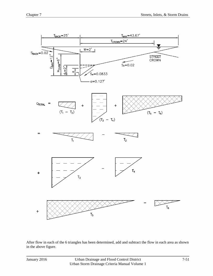
Chapter 7 Streets, Inlets, & Storm Drains
January 2016 Urban Drainage and Flood Control District 7-51 Urban Storm Drainage Criteria Manual Volume 1
After flow in each of the 6 triangles has been determined, add and subtract the flow in each area as shown in the above figure.
Streets, Inlets, & Storm Drains Chapter 7
7-52 Urban Drainage and Flood Control District January 2016 Urban Storm Drainage Criteria Manual Volume 1
654321 TTTTTT QQQQQQQ −+−+−=
( )( )( )3/82/13/51 2501.002.0
013.056.0
=TQ = 33.9 cfs
( )( )( )3/82/13/52 1501.002.0
013.056.0
=TQ = 8.86 cfs
( )( )( )3/82/13/53 1201.00833.0
013.056.0
=TQ = 51.7 cfs
( )( )( )3/82/13/54 1001.00833.0
013.056.0
=TQ = 31.8 cfs
(Solve for T using equation 7-9)
( )( )( )3/82/13/55 7.4101.002.0
016.056.0
=TQ = 107.8 cfs
( )( )( )3/82/13/56 7.1901.002.0
016.056.0
=TQ = 14.6 cfs
Therefore by combining the above calculations the total flow can be calculated as:
654321 TTTTTT QQQQQQQ −+−+−= = 138 cfs
Note: UD-Inlet.xls uses HEC-22 methodology to solve this problem and will provide a slightly different answer.
6.4 Example—V-Shaped Swale Capacity
Determine the maximum discharge and depth of flow in a V-shaped, roadside grass swale with side slopes of 8% and 6%, a longitudinal slope of 2% and a total width of 6 feet.
The adjusted slope, Sx, is determined using Equation 7-13:
21
21
xx
xxx SS
SSS+
=
06.008.0)06.0)(08.0(
+=xS = 0.034
From Equation 7-1, the flow through the swale is computed:
3/82/13/556.0 TSSn
Q ox=
Chapter 7 Streets, Inlets, & Storm Drains
January 2016 Urban Drainage and Flood Control District 7-53 Urban Storm Drainage Criteria Manual Volume 1
3/82/13/5 602.0034.003.056.0
=Q = 1.12 cfs
Using Equation 7-2 the flow depth is calculated as:
xTSy =
)034.0(6=y =0.2 feet
6.5 Example—V-Shaped Swale Design
Design a V-shaped swale to convey a flow of 1.8 cfs. The available swale top width is 8 feet, the longitudinal slope is 1%, and the Manning’s roughness factor is 0.16. Determine the cross slopes and the depth of the swale.
Solving Equation 7-1 for Sx (i.e., average side slope) yields:
= 0.024 ft/ft
Now Equation 7-13 is used to solve for the actual cross slope assuming Sx1 = Sx2 , Equation 7-13 can be rewritten and solved for Sx1 :
xSS 2= = 2(0.024) = 0.048 ft/ft
Then using Equation 7-2 yields a flow depth, y, of:
xTSy = = (0.024)(8) = 0.19 feet
The swale is 8-feet wide with right and left side slopes of 0.048 ft/ft and a flow depth of 0.19 feet.
5/3
3/82/1 8)01.0(56.0016.0)8.1(
=xS
5/3
3/82/156.0
=
TSQnS
ox

Streets, Inlets, & Storm Drains Chapter 7
7-54 Urban Drainage and Flood Control District January 2016 Urban Storm Drainage Criteria Manual Volume 1
6.6 Example—Grate Inlet Capacity
Determine the efficiency of a CDOT Type C Standard Grate (W = 2 feet and L = 2 feet) when placed in a composite gutter section with a 2-foot concrete gutter that has a 2-inch drop between the gutter lip and gutter flowline. The street cross slope is 2% and the longitudinal slope of 1%. The flow in the gutter is 2.5 cfs with a spread of 8.5 feet.
Using Equation 7-7, determine the ratio of gutter flow to total flow (Qw/Q) (represented by Eo):
11)/(
/1
/1
1
3/8
−
−
+
+=
WTSSSSE
xw
xwO
0.66
11)2/5.8(
02.0/083.01
02.0/083.01
1
3/8
=
−
−
+
+=OE
Solve Equation 7-6 for Qx to determine the flow in the section outside of the depressed gutter:
( )ox EQQ −= 1 = 2.5(1-0.66) = 0.85 cfs
The flow in the dressed gutter section is determined by subtracting this value from the total flow:
65.185.05.2 =−=wQ cfs
Next, find the flow area using Equation 7-10 and velocity using the continuity equation V = Q/A.
2
2 aWTSA x +=
2)2(127.0)5.8(02.0 2 +
=A = 0.85 ft2
85.05.2
==AQV =2.94 fps
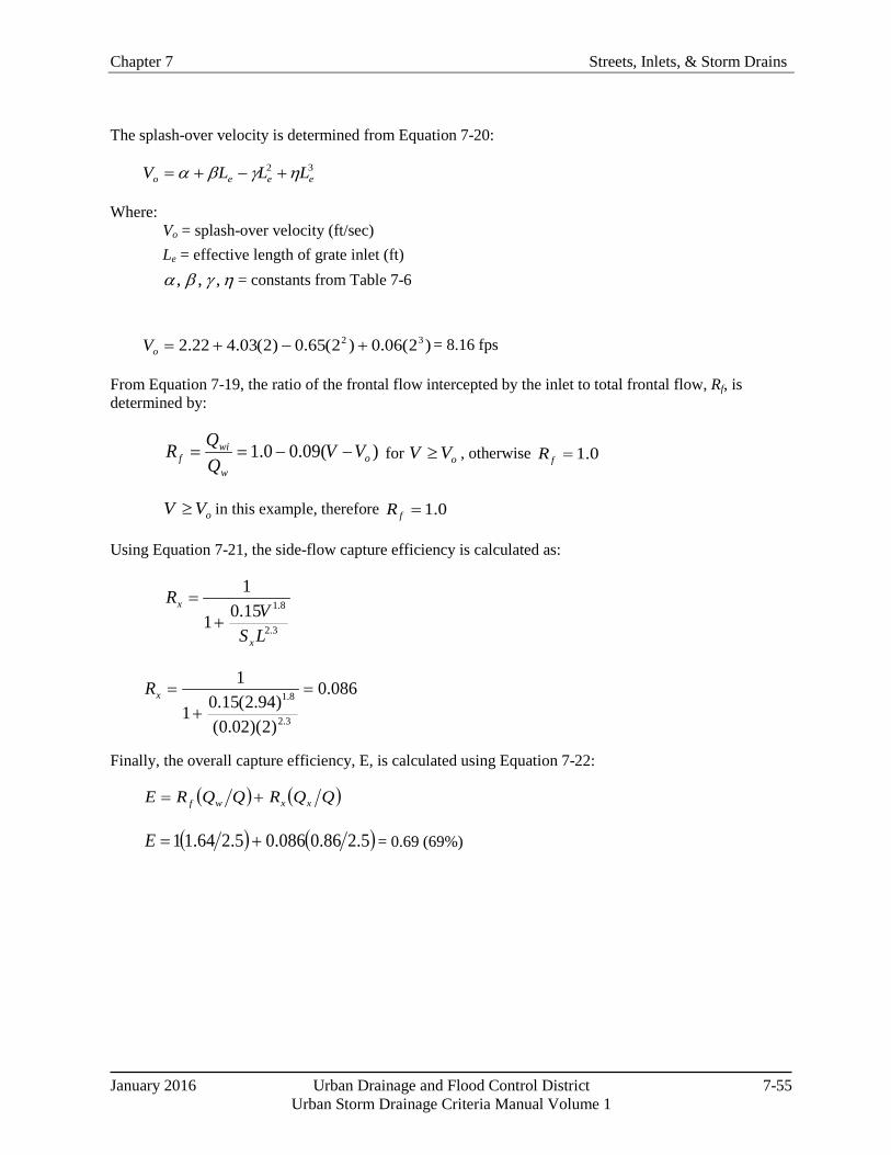
Chapter 7 Streets, Inlets, & Storm Drains
January 2016 Urban Drainage and Flood Control District 7-55 Urban Storm Drainage Criteria Manual Volume 1
The splash-over velocity is determined from Equation 7-20:
32eeeo LLLV ηγβα +−+=
Where: Vo = splash-over velocity (ft/sec) Le = effective length of grate inlet (ft)
= constants from Table 7-6
)2(06.0)2(65.0)2(03.422.2 32 +−+=oV = 8.16 fps
From Equation 7-19, the ratio of the frontal flow intercepted by the inlet to total frontal flow, Rf, is determined by:
)(09.00.1 ow
wif VV
QQR −−== for oVV ≥ , otherwise 0.1=fR
oVV ≥ in this example, therefore 0.1=fR
Using Equation 7-21, the side-flow capture efficiency is calculated as:
3.2
8.115.01
1
LSV
R
x
x
+=
086.0
)2)(02.0()94.2(15.01
1
3.2
8.1 =+
=xR
Finally, the overall capture efficiency, E, is calculated using Equation 7-22:
( ) ( )QQRQQRE xxwf +=
( ) ( )5.286.0086.05.264.11 +=E = 0.69 (69%)
ηγβα ,,,
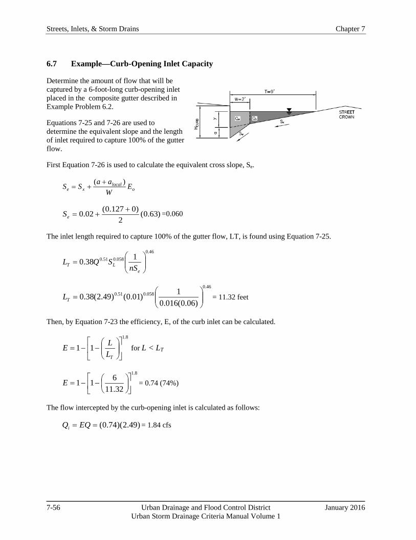
Streets, Inlets, & Storm Drains Chapter 7
7-56 Urban Drainage and Flood Control District January 2016 Urban Storm Drainage Criteria Manual Volume 1
6.7 Example—Curb-Opening Inlet Capacity
Determine the amount of flow that will be captured by a 6-foot-long curb-opening inlet placed in the composite gutter described in Example Problem 6.2.
Equations 7-25 and 7-26 are used to determine the equivalent slope and the length of inlet required to capture 100% of the gutter flow.
First Equation 7-26 is used to calculate the equivalent cross slope, Se.
olocal
xe EWaaSS )( +
+=
)63.0(2
)0127.0(02.0 ++=eS =0.060
The inlet length required to capture 100% of the gutter flow, LT, is found using Equation 7-25.
46.0058.051.0 138.0
=
eLT nS
SQL
46.0058.051.0
)06.0(016.01)01.0()49.2(38.0
=TL = 11.32 feet
Then, by Equation 7-23 the efficiency, E, of the curb inlet can be calculated.
8.1
11
−−=
TLLE for L < LT
8.1
32.11611
−−=E = 0.74 (74%)
The flow intercepted by the curb-opening inlet is calculated as follows:
)49.2)(74.0(== EQQi = 1.84 cfs

Chapter 7 Streets, Inlets, & Storm Drains
January 2016 Urban Drainage and Flood Control District 7-57 Urban Storm Drainage Criteria Manual Volume 1
6.8 Example—Design of a Network of Inlets Using UD-Inlet
Determine the number of CDOT Type R curb inlets needed to maintain allowable street flow for the 5-yr and 100-year storm events for each side of the street as shown in the below figure. The area can be described as a 4.8-acre residential development in Denver with LT = 711 ft, channel length LC = 637 ft, WT = 310 ft. and WS = 30 ft. Each lot is 0.25 acres. The development has imperviousness I=75% and type C soil. The channel slope is 2% and the overland slope is 3%. All flows must be contained within the street and gutter section (i.e., no flow behind the curb). Additionally, the flow spread for the minor storm shall not exceed 9 ft.
The tributary area to be used is half of the total development (A = 2.4 acre). Based on the dimensions of the lot sizes, the overland flow length is 136 ft. Use the Q-Peak tab of the UD-Inlet workbook to calculate the 5-year and 100-year peak flow for the upper portion of the tributary area. This requires approximation of the location of the most upstream inlet and calculation of the area tributary to this inlet. The following screenshot shows the Q-Peak input and output for the upper 0.7 acres of the tributary area. Based on the geometry of the development, this corresponds to a channel flow length of 157 feet.

Streets, Inlets, & Storm Drains Chapter 7
7-58 Urban Drainage and Flood Control District January 2016 Urban Storm Drainage Criteria Manual Volume 1
The Q-Peak inlet calculates the 5-year and 100-year peak flow based on the estimated sub-catchment area to the first inlet, percent imperviousness, soil type, appropriate time of concentration calculations, as well as location-specific rainfall information and runoff coefficients. For this problem, the 5-year flow is 2.1 cfs and the 100-year flow is 4.8 cfs. Alternatively, the user could enter known flows in this tab. Once the flows have been calculated, press the “Add Results to New Inlet” button. This adds a new inlet to the Inlet Management tab and opens a new tab for calculation of both the flow spread and depth in the street and the design of the receiving inlet.
On the inlet tab, enter the geometry of half of the street section. Use the requirements stated in the problem statement for the allowable spread and depth of flow. This section indicates the maximum street flow for the minor and major storm events based on allowable spread and depth criteria. If the allowable street flow is less than the flow calculated on the Q-Peak tab, reduce the area and associated channel length on the Q-Peak tab. For this example, neither flow depth nor flow spread exceed criteria. See the screenshot below.
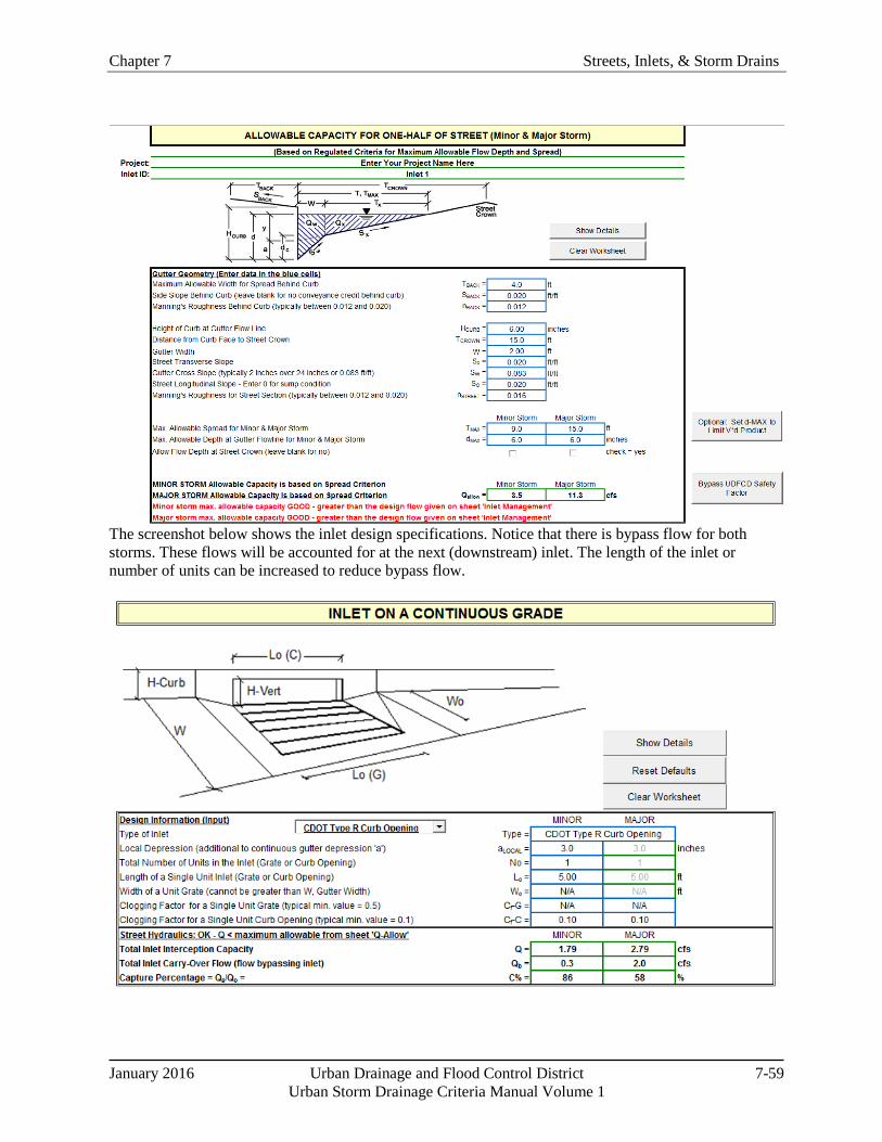
Chapter 7 Streets, Inlets, & Storm Drains
January 2016 Urban Drainage and Flood Control District 7-59 Urban Storm Drainage Criteria Manual Volume 1
The screenshot below shows the inlet design specifications. Notice that there is bypass flow for both storms. These flows will be accounted for at the next (downstream) inlet. The length of the inlet or number of units can be increased to reduce bypass flow.
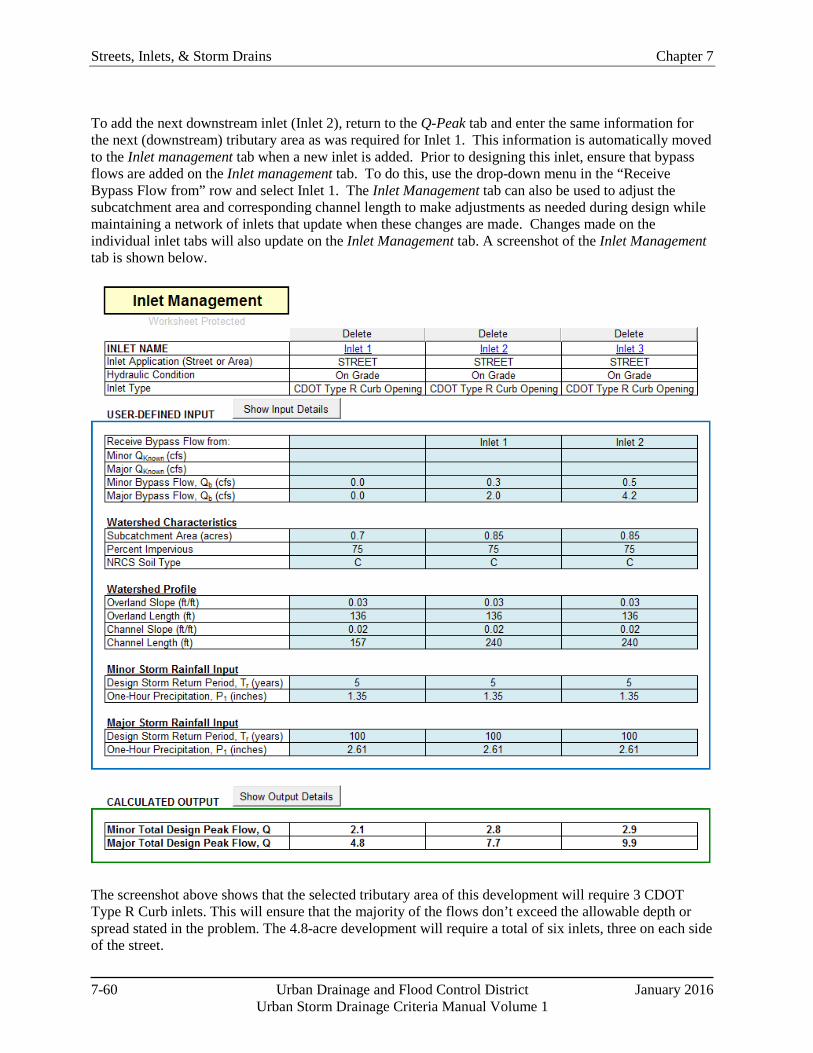
Streets, Inlets, & Storm Drains Chapter 7
7-60 Urban Drainage and Flood Control District January 2016 Urban Storm Drainage Criteria Manual Volume 1
To add the next downstream inlet (Inlet 2), return to the Q-Peak tab and enter the same information for the next (downstream) tributary area as was required for Inlet 1. This information is automatically moved to the Inlet management tab when a new inlet is added. Prior to designing this inlet, ensure that bypass flows are added on the Inlet management tab. To do this, use the drop-down menu in the “Receive Bypass Flow from” row and select Inlet 1. The Inlet Management tab can also be used to adjust the subcatchment area and corresponding channel length to make adjustments as needed during design while maintaining a network of inlets that update when these changes are made. Changes made on the individual inlet tabs will also update on the Inlet Management tab. A screenshot of the Inlet Management tab is shown below.
The screenshot above shows that the selected tributary area of this development will require 3 CDOT Type R Curb inlets. This will ensure that the majority of the flows don’t exceed the allowable depth or spread stated in the problem. The 4.8-acre development will require a total of six inlets, three on each side of the street.

Chapter 7 Streets, Inlets, & Storm Drains
January 2016 Urban Drainage and Flood Control District 7-61 Urban Storm Drainage Criteria Manual Volume 1
7.0 References Akan, A.O. and R.J. Houghtalen. 2002. Urban Hydrology, Hydraulics, and Water Quality. Upper Saddle River, NJ: Prentice Hall. Forthcoming.
Colorado State University (CSU). 2009. Hydraulic Efficiency of Grate and Curb Inlets for Urban Storm Drainage. Denver, CO: Urban Drainage and Flood Control District.
Federal Highway Administration (FHWA). 1984. Drainage of Highway Pavements. Hydraulic Engineering Circular 12. McLean, VA: Federal Highway Administration.
Federal Highway Administration (FHWA). 2009. Urban Drainage Design Manual. Hydraulic Engineering Circular 22. Washington, DC: Federal Highway Administration.
Guo, J.C.Y. 1992. Technical Manual for Computer Model UDSEWER for Storm Sewer System Design. Denver, CO: Department of Civil Engineering, University of Colorado at Denver.
Guo, J.C.Y. 1998a. Storm Sewer System Design and Flow Analysis Using the Personal Computer Model UDSEWER. Denver, CO: Urban Drainage and Flood Control District.
Guo, J.C.Y. 1998b. Street Hydraulics and Inlet Sizing Using the Computer Model UDINLET. Denver, CO: Urban Drainage and Flood Control District.
Guo, J.C.Y. 1999. Storm Water System Design. CE 5803, University of Colorado at Denver.
Guo, J.C.Y. 2000a. Design of Grate Inlets with a Clogging Factor. Advances in Environmental Research 4(3)181-186.
Guo, J.C.Y. 2000b. Street Storm Water Conveyance Capacity. Journal of Irrigation and Drainage Engineering 136(2)119-124.
Wright-McLaughlin Engineers. 1969. Urban Storm Drainage Criteria Manual. Prepared for the Denver Regional Council of Governments. Denver, CO: Urban Drainage and Flood Control District.