7.1

Chapter 7. SOIL COMPONENT

E.E. Alberts, M.A. Nearing, M.A. Weltz, L.M. Risse,F.B. Pierson, X.C. Zhang, J.M. Laflen and J.R. Simanton

7.1 Introduction and Objectives

Soil properties influence the basic water erosion processes of infiltration and surface runoff, soildetachment by raindrops and concentrated flow, and sediment transport. The purpose of this chapter is toprovide the WEPP user with background information on the soil and soil-related variables currentlypredicted in the WEPP model.

7.2 Background

7.2.1 Hydrology Parameters

Four soil variables that influence the hydrology portion of the erosion process are predicted in thiscomponent, including: 1) random roughness, 2) ridge height, 3) bulk density, and 4) effective hydraulicconductivity. Random roughness is most often associated with tillage of cropland soil, but any tillage orsoil disturbing operation creates soil roughness. Ridge height, which is a form of oriented roughness,results when the soil is arranged in a regular way by a tillage implement and varies by a factor of two ormore depending upon implement type. Depressional storage of rainfall and hydraulic resistance tooverland flow are positively correlated with soil roughness. Soil roughness changes temporarily due totillage, rainfall weathering, and freezing and thawing. Bulk density reflects the total pore volume of thesoil and is used to predict several infiltration parameters, including wetting front suction. Bulk densitychanges temporally due to tillage, wetting and drying, and freezing and thawing. Adjustments to bulkdensity are needed to account for factors such as the volumes of entrapped air and coarse fragments in thesoil.

7.2.2 Soil Detachment Parameters

Interrill erodibility (Ki) is a measure of sediment delivery rate to rills as a function of rainfallintensity and runoff rate. For cropland and rangeland soils, base Ki values were predicted fromrelationships developed from field experiments conducted in 1987 and 1988 (Laflen et al., 1987;Simanton et al., 1987). Base Ki values for cropland soils are measured when the soil is in a loose,unconsolidated condition typical of that found after primary and secondary tillage using conventionaltillage practices. Base Ki values for rangeland are measured on undisturbed soils with all vegetation andcoarse fragments removed. Base Ki values for cropland and rangeland soils need to be adjusted forfactors that influence the resistance of the soil to detachment, such as live and dead root biomass, soilfreezing and thawing, and mechanical and livestock compaction.

Rill erodibility (Kr) is a measure of soil susceptibility to detachment by concentrated flow, and isoften defined as the increase in soil detachment per unit increase in shear stress of clear water flow.Critical shear stress (τc) is an important term in the rill detachment equation, and is the shear stress belowwhich no soil detachment occurs. Critical shear stress (τc) is the shear intercept on a plot of detachmentby clear water vs. shear stress in rills. Rate of detachment in rills may be influenced by a number ofvariables including soil disturbance by tillage, living root biomass, incorporated residue, soilconsolidation, and freezing and thawing.

7.3 User and Climatic Inputs

The number of overland flow elements (OFEs) existing on the hillslope profile is specified by theuser, with an OFE being defined as an area of uniform cropping, management, and soil characteristics.

July 1995

7.2

Soil information at the mapping unit level is stored in a soil input file. If the hillslope segment begins ona ridge and ends in a alluvial valley, the location of each mapping unit can be specified and soil propertiesof each read into the model from the soil input file. Mapping units on the hillslope profile are specified tobetter predict the effects of basic soil physical and chemical properties on infiltration and soil erodibilityparameters.

Because tillage is one major process altering soil properties, the user must specify information onany tillage operation that occurs during the erosion simulation. Specific inputs include: 1) implementtype, 2) tillage date, 3) tillage depth, 4) surface disturbance level, and 5) residue burial amounts.

After tillage, temporal changes in soil roughness, bulk density, and hydraulic conductivity occurdue to soil wetting and drying and freezing and thawing. Daily rainfall, max-min air temperatures, andsoil water content are important variables in some equations that predict temporal soil properties.

7.4 Time Invariant Soil Properties

Time invariant soil properties are used to calculate baseline soil infiltration and erodibilityparameters. Most baseline soil infiltration and erodibility parameters are calculated internal to the modelusing data read in from the soil input file (see User Summary for more information).

7.5 Random Roughness

Random roughness following a tillage operation is estimated based upon measured averages for animplement, which is similar to the approach used in EPIC (Williams et al., 1984). Table 7.5.1 shows therandom roughness value assigned to each tillage implement in the current crop management input file.

RRo and RHo are random roughness and ridge height parameters. RINT represents the on-centerridge interval.

Soil random roughness immediately after a tillage operation is predicted from:

RRi = RRo Tds + RRt −1RQ1 − Tds

HP

[7.5.1]

where RRi is the random roughness immediately after tillage (m), RRo is the random roughness created bya tillage implement, RRt −1 is the random roughness of the soil surface on the day previous to the tillageoperation, and Tds is the fraction of the soil surface disturbed by the tillage implement. This approachaccounts for the effect of prior random roughness on random roughness after tillage.

Random roughness decay with time after tillage is predicted from a modified relationship of Potter(1990):

RRt = RRi e−Cbr

IJL b

RchhhMJO

0.6

[7.5.2]

where RRt is the random roughness at time t (m), Cbr is the adjustment factor for buried residue, Rc is thecumulative rainfall since tillage (m), and b is a coefficient. Cbr is predicted by:

Cbr = 1 − 0.5 br [7.5.3]

where br is the mass of the buried residue in the 0-to 0.15-meter soil zone (kg .m−2). Cbr is arbitrarily setto be no less the 0.3 in the WEPP model. The adjustment assumes that the buried residue reduces thesurface roughness decay rate. The coefficient b is computed as:

July 1995

7.3

Table 7.5.1. WEPP soil parameters for 78 tillage implements.iiiiiiiiiiiiiiiiiiiiiiiiiiiiiiiiiiiiiiiiiiiiiiiiiiiiiiiiiiiiiiiiiiiiiiiiiiiiiiiiiiiiiiiiiiiiii

WEPP Parameter ValuesIMPLEMENT CODE & DESCRIPTION RRo Tds RHo RINT TDMEAN

(m) (m) (m) (m)iiiiiiiiiiiiiiiiiiiiiiiiiiiiiiiiiiiiiiiiiiiiiiiiiiiiiiiiiiiiiiiiiiiiiiiiiiiiiiiiiiiiiiiiiiiiiiANHYDISK - anhydrous applicator with closing disks 0.013 0.25 0.025 0.75 0ANHYDROS - anhydrous applicator 0.013 0.15 0.025 0.75 0BEDDER - bedders, lister and hippers 0.025 1 0.15 0.75 0.1CHISCOST - chisel plow with coulters and straight chisel spikes 0.023 1 0.05 0.3 0.15CHISCOSW - chisel plow with coulters and sweeps 0.023 1 0.05 0.3 0.15CHISCOTW - chisel plow with coulters and twisted points or shovels 0.026 1 0.075 0.3 0.15CHISELSW - chisel plow with sweeps 0.023 1 0.05 0.3 0.15CHISSTSP - chisel plow, straight with spike points 0.023 1 0.05 0.3 0.15CHISTPSH - chisel plow, twisted points or shovels 0.026 1 0.075 0.3 0.15COMBDISK - combination tools with disks, shanks and leveling atchmnts 0.015 1 0.025 0.3 0.075COMBSPRG - combination tools with spring teeth and rolling basket 0.015 1 0.025 0.3 0.075CRNTFRR - drill, no-till in flat residues-ripple or bubble coulters 0.012 0.5 0.025 0.2 0CULTFW - cultivator, row finger wheels 0.015 0.95 0.05 0.75 0.025CULTMUSW - cultivator, row, multiple sweeps per row 0.015 0.85 0.075 0.75 0.05CULTRD - cultivator, row, rolling disks 0.015 0.9 0.15 0.75 0.05CULTRT - cultivator, row, ridge till 0.015 0.9 0.15 0.75 0.05CULTSW - cultivator, row, single sweep per row 0.015 0.85 0.075 0.75 0.05DI1WA12+ - disk, one-way with 12-16" blades 0.026 1 0.05 0.2 0.1DI1WA18+ - disk, one-way with 18-30" blades 0.026 1 0.05 0.2 0.1DICHSP - disk chisel plow with straight chisel spike pts 0.026 1 0.075 0.3 0.15DICHSW - disk chisel plow with sweeps 0.023 1 0.05 0.3 0.15DICHTW - disk chisel plow with twisted points or shovels 0.026 1 0.075 0.3 0.15DIOFF10 - disk, offset-heavy plow > 10" spacing 0.038 1 0.05 0.2 0.1DIOFF9 - disk, offset-primary cutting > 9" spacing 0.038 1 0.05 0.2 0.1DIOFFFIN - disk, offset, finishing 7-9" spacing 0.038 1 0.05 0.2 0.075DIPLOW - disk plow 0.038 1 0.05 0.2 0.1DISGANG - disk, single gang 0.026 1 0.05 0.2 0.05DITAF19 - disk, tandem-finishing 7-9" spacing 0.026 1 0.05 0.2 0.05DITAHP10 - disk, tandem-heavy plowing > 10" spacing 0.026 1 0.05 0.2 0.075DITALIAH - disk, tandem-light after harvest, before other tillage 0.026 1 0.05 0.2 0.025DITAPR9 - disk, tandem-primary cutting > 9" spacing 0.026 1 0.05 0.2 0.075DRDDO - drill with double disk opener 0.012 0.85 0.025 0.2 0.025DRDF12- drill, deep furrow with 12" spacing 0.012 0.9 0.05 0.2 0.075DRHOE - drill, hoe opener 0.012 0.8 0.05 0.2 0.025DRNTFLSC - drill, no-till in flat residues-smooth coulters 0.012 0.4 0.025 0.2 0DRNTFRFC - drill, no-till in flat residues-fluted coulters 0.012 0.6 0.025 0.2 0DRNTSRFC - drill, no-till in standing stubble-fluted coulters 0.012 0.6 0.025 0.2 0DRNTSRRI - drill, no-till in standing stubble-ripple or bubble coulters 0.012 0.5 0.025 0.2 0DRNTSRSC - drill, no-till in standing stubble-smooth coulters 0.012 0.4 0.025 0.2 0DRSDFP7+ - drill, semi-deep furrow or press 7-12" spacing 0.012 0.9 0.05 0.2 0.05DRSDO - drill, single disk opener (conventional) 0.012 0.85 0.05 0.2 0.025FCPTDP - field cultivator, primary tillage-duckfoot points 0.015 1 0.025 0.3 0.075FCPTS12+ - field cultivator, primary tillage-sweeps 12-20" 0.015 1 0.025 0.3 0.075FCPTSW6+ - field cultivator, primary tillage-sweeps or shovels 6-12" 0.015 1 0.025 0.3 0.075FCSTACDP - field cultivator, secondary tillage, after duckfoot points 0.015 1 0.025 0.3 0.05

July 1995

7.4

FCSTACDS - field cultivator, secondary tillage, sweeps 12-20" 0.015 1 0.025 0.3 0.05FCSTACSH - field cultivator, secondary tillage, swp or shov 6-12" 0.015 1 0.025 0.3 0.05FURROWD - furrow diker 0.015 0.7 0.025 0.75 0.05HAFTT - harrow-flex-tine tooth 0.018 1 0.025 0.1 0.025HAPR - harrow-packer roller 0.01 1 0.025 0.08 0.025HARHCP - harrow-roller harrow (cultipacker) 0.01 1 0.025 0.08 0.025HASP - harrow-spike tooth 0.015 1 0.025 0.05 0.025HASPTCT - harrow-springtooth (coil tine) 0.015 1 0.025 0.05 0.025MANUAPPL - applicator, subsurface manure 0.013 0.4 0.025 0.75 0MOPL - plow, moldboard, 8" 0.043 0.1 0.05 0.4 0.15MOPLUF - plow, moldboard with uphill furrow (Pacific NW only) 0.043 1 0.05 0.4 0.15MULCHT - mulch treader 0.015 1 0.025 0.05 0.025PARAPLOW - paratill/paraplow 0.01 0.3 0.025 0.36 0.2PLDDO - planter, double disk openers 0.012 0.15 0.025 0.75 0.05PLNTFC - planter, no-till with fluted coulters 0.012 0.15 0.025 0.75 0PLNTRC - planter, no-till with ripple coulters 0.012 0.15 0.025 0.75 0PLNTSC - planter, no-till with smooth coulters 0.012 0.15 0.025 0.75 0PLRO - planter, runner openers 0.013 0.2 0.025 0.75 0.05PLRT - planter, ridge-till 0.013 0.4 0.1 0.75 0.05PLSDDO - planter, staggered double disk openers 0.013 0.15 0.025 0.75 0.05PLST2C - planter, strip-till with 2 or 3 fluted coulters 0.013 0.3 0.025 0.75 0.05PLSTRC - planter, strip-till with row cleaning devices (8-14" wide) 0.013 0.4 0.025 0.75 0.05RORRP - rodweeder, plain rotary rod 0.01 1 0.025 0.13 0.05RORRSC - rodweeder, rotary rod with semi-chisels or shovels 0.01 1 0.025 0.13 0.05ROTHOE - rotary hoe 0.012 1 0 0 0.025ROTILPO - rotary tiller-primary operation 6" deep 0.015 1 0 0 0.15ROTILSO - rotary tiller-secondary operation 3" deep 0.015 1 0 0 0.075ROTILST - rotary tiller, strip tillage - 12" tilled on 40" rows 0.015 0.3 0 0 0.075SUBCC - subsoil-chisel, combination chisel 0.015 1 0.075 0.3 0.4SUBCD - subsoiler, combination disk 0.015 1 0.075 0.3 0.4SUBVRIP - subsoiler, V ripper 20" spacing 0.015 0.2 0.075 0.5 0.4UNSMWBL - undercutter, stubble-mulch sweep (20-30"wide) or blade 0.015 1 0.075 1 0.075UNSMWBP - undercutter, stubble-mulch sweep or blade plows > 30" wide 0.015 1 0.075 1.5 0.075iiiiiiiiiiiiiiiiiiiiiiiiiiiiiiiiiiiiiiiiiiiiiiiiiiiiiiiiiiiiiiiiiiiiiiiiiiiiiiiiiiiiiiiiiiiiii

b = 63 + 62.7 ln (50 orgmat) + 1570 clay − 2500 clay 2 [7.5.4]

where orgmat is the soil organic matter content (0-1), and clay is the soil clay content (0-1). Only the Cbrcoefficient and its associated equation were added to the Potter (1990) equation.

Since WEPP assumes that surface roughness in a rill is relatively small and is also independent ofroughness in interrill, friction due to form roughness is not included in the total friction factor of the rill.This is reasonable only after the rill has formed. But during rill initiation stage, surface roughness shouldbe considered. It is expected that rill formation should be slower on a rougher surface than on a smootherone. This can be realized by relating critical shear (τc) to RR, because WEPP assumes that rill erosionwill not be initiated until flow shear exceeds the critical shear. By calibration, the following equation wasobtained:

Cτrr = 1.0 + 8.0 (RRt − 0.006) [7.5.5]

where Cτrr is the adjustment factor, and 0.006 is the minimum RR value in meters. τc is multiplied byCτrr , thus τc increases as RR increases, which reduces rill detachment.

July 1995

7.5

Table 7.5.1 contains the recommended values for five tillage parameters - RRo (random roughness)immediately after tillage, Tds (fraction of soil surface disturbed by the tillage implement), RHo (ridgeheight immediately after tillage), RINT (ridge interval), and TDMEAN (the mean tillage depth associatedwith each implement). See Chapter 9 for information on tillage implement effects on residue burial.

7.6 Ridge Height

A ridge height value is assigned to a tillage implement based upon measured averages for eachimplement (see Table 7.5.1 for assigned ridge height values), which is similar to the approach used inEPIC (Williams et al., 1984).

Ridge height decay following tillage is predicted from:

RHt = RHo e−Cbr

IJL b

RchhhMJO

0.6

[7.6.1]

where RHt is the ridge height (m) at time t, RHo is the ridge height immediately after tillage (m), and Cbr ,Rc, and b are as defined in section 7.5.

Large ridges made by a ridging cultivator or a similar ridging implement do not decay as fast assmaller ridges made by a disk or chisel plow. Criteria used to identify a well-defined ridge-furrow systemis that ridge height after tillage for any implement in the tillage sequence is ≥ 0.1 m and the ridge intervalis between 0.6 and 1.4 meters. For this condition, ridge height is not allowed to decay below 0.1 m.

7.7 Bulk Density

7.7.1 Tillage Effects

Soil bulk density changes are used to predict changes in infiltration parameters. Bulk density aftertillage is difficult to predict because of limited knowledge, particularly for point- and rolling-typeimplements, of how an implement interacts with a soil as influenced by tillage speed, tillage depth, andsoil cohesion.

The approach chosen to account for the influence of tillage on soil bulk density is to use aclassification scheme where each implement is assigned a tillage disturbance value from 0 to 1, which issimilar to the approach used in EPIC (Williams et al., 1984). The concept is based, in part, on measuredeffects of various tillage implements on residue cover (see tillage intensity values in Chapter 9).

The equation used to predict soil bulk density after tillage is (Williams et al., 1984):

ρt = ρt −1 −RJQ

ILρt −1 − 0.667 ρc

MO Tds

HJP

[7.7.1]

where ρt is the bulk density after tillage (kg .m−3), ρt −1 is the bulk density before tillage (kg .m−3), ρc isthe consolidated soil bulk density (kg .m−3) at 0.033 MPa of tension, and Tds is the fraction of the soilsurface disturbed by the tillage implement (0-1).

Consolidated soil bulk density, ρc, is calculated by the model from the soil input data from therelationship:

ρc = (1.514 + 0.25 sand − 13.0 sand orgmat − 6.0 clay orgmat − 0.48 clay CECr) 103 [7.7.2]

where ρc is the consolidated soil bulk density (kg .m−3) at 0.033 MPa of tension, sand is the sand content(0-1), orgmat is the organic matter content (0-1), clay is the clay content (0-1), and CECr is the ratio ofthe cation exchange capacity of the clay (CECc) to the clay content of the soil.

July 1995

7.6

The cation exchange capacity of the clay fraction of the soil is calculated from:

CECc = CEC − orgmat (142 + 170 Dg) [7.7.3]

where CEC is the cation exchange capacity of the soil (meq /100g) and Dg is the average depth of thehorizon of interest (m).

The WEPP model currently assumes the depth of primary tillage to be 0.2 meters and the depth ofsecondary tillage to be 0.1 meters. The model uses the information in the soil input file to create a newset of soil layers which are appropriate for use in the infiltration and percolation computations. The topsoil layer has a thickness of 0.1 meters, and the second soil layer also has a thickness of 0.1 meters. Allremaining soil layers to a total maximum possible depth of 1.8 meters have a thickness of 0.2 meters.Soil properties for the newly-created layers are obtained by using weighted averages of input soilproperties from the corresponding depths. All processes that influence soil bulk density are modeledwithin the primary and secondary tillage zones.

7.7.2 Soil Water Content Effects

The bulk density of the soil at the wilting point, ρd , is predicted from:

ρd = RQ−0.024 +0.001 ρc +1.55 clay CECr +clay 2 CECr

2 −1.1 CECr2 clay −1.4 orgmat H

P 103 [7.7.4]

The residual water content of the soil is predicted from (Baumer, personal communication):

θr = (0.000002 + 0.0001 orgmat + 0.00025 clay CECr0.45) ρt

[7.7.5]

where θr is the residual volumetric water content of the soil (m3.m−3).

The volumetric water content at 0.033 MPa of tension (field capacity), θfc , is predicted from:

θfc = 0.2391 − 0.19 sand + 2.1 orgmat + 0.72 θd[7.7.6]

The volumetric water content at 1.5 MPa of tension (wilting point), θd , is predicted from:

θd =0.0022 +0.383 clay −0.5 clay 2 sand 2 +0.265 clay CECr2 − (0.06 clay 2 +0.108 clay)

IJL 1000

ρthhhhhMJO

2[7.7.7]

7.7.3 Rainfall Consolidation

Rainfall on freshly-tilled soil consolidates it and increases soil bulk density. Soil bulk densityincreases by rainfall are predicted from (Onstad et al., 1984):

ρd = ρt + ∆ ρrf[7.7.8]

where ρd is the bulk density after rainfall (kg .m−3), ρt is the bulk density after tillage (kg .m−3), and ∆ρrfis the bulk density increase due to consolidation by rainfall (kg .m−3).

The increase in soil bulk density from rainfall consolidation (∆ρrf) is calculated from:

∆ ρrf = ∆ ρmx 0.01 + Rc

Rchhhhhhhhh [7.7.9]

July 1995

7.7

where ∆ρmx is the maximum increase in soil bulk density with rainfall and Rc is the cumulative rainfallsince tillage (m).

The maximum increase in soil bulk density with rainfall is predicted from:

∆ ρmx = 1650 − 2900 clay + 3000 clay 2 − 0.92 ρt[7.7.10]

and if ∆ρmx is ≤0.0, then ∆ρmx= 0.0.

The upper boundary for soil bulk density change with rainfall is reached after a freshly-tilled soilreceives 0.1 m of rainfall.

7.7.4 Weathering Consolidation

For most soils, 0.1 m of rainfall does not fully consolidate the soil. Consolidated soil bulk density(ρc) is assumed to be the upper boundary to which a soil naturally tends to consolidate.

The difference between the naturally consolidated bulk density and the bulk density after 0.1 m ofrainfall is:

∆ ρc = ρc − ρt[7.7.11]

where ∆ρc is the difference in soil bulk density between a soil that is naturally consolidated and one thathas received 0.1 m of rainfall. ρt is soil bulk density on the day cumulative rainfall since tillage equals0.1 m.

The adjustment for increasing bulk density due to weathering and longer-term soil consolidation iscomputed from:

∆ ρwt = ∆ρc Fdc[7.7.12]

where ∆ρwt is the daily increase in soil bulk density (kg .m−3) after 0.1 m of rainfall, and Fdc is the dailyconsolidation factor.

The daily bulk density consolidation factor is predicted from:

Fdc = 1 − e−0.005 daycnt [7.7.13]

where daycnt is a counter to keep track of the number of days since the last tillage operation.

Soil bulk density changes following tillage are predicted from:

ρt = ρt −1 + ∆ ρrf + ∆ ρwt[7.7.14]

where the tillage occurred the previous day (t −1) and the variables have been previously described.

7.8 Porosity

Total soil porosity (φt) is predicted from soil bulk density by:

φt = 1 − ρt /2650 [7.8.1]

where ρt is the bulk density (kg .m−3) at time t.

The volume of entrapped air in the soil (Fa) is calculated from (Baumer, personal communication):

July 1995

7.8

Fa = 1.0 −100

3.8 + 1.9 clay 2 − 3.365 sand + 12.6 CECr clay + 100 orgmat (sand/2)2hhhhhhhhhhhhhhhhhhhhhhhhhhhhhhhhhhhhhhhhhhhhhhhhhhhhhhhhhhh [7.8.2]

where the clay, sand, and organic matter contents of the soil are given as a fraction (0-1).

The correction for the volume of coarse fragments in the soil (Fcf) is predicted from (Brakensiek etal., 1986):

Fcf = 1 − Vcf[7.8.3]

Vcf is the fraction of coarse fragments by volume (0-1) and is predicted from:

Vcf =2.65 I

L1 − Mcf

MO

Mcf 1000

ρthhhhhhhhhhhhhhhhhh [7.8.4]

where Mcf is the fraction of coarse fragments by weight (0-1).

The effective porosity of the soil (φe) is calculated from the total porosity determined from soilbulk density (< 2-mm material) and adjusted for the volume of coarse fragments and the volume ofentrapped air. φe is computed from:

φe = φt Fa Fcf[7.8.5]

Volumetric soil water contents at 0.020, 0.033, and 1.5 MPa are adjusted for the volumes ofentrapped air (Fa) and coarse fragments (Fcf). The adjusted soil parameters are then used in soil waterstorage computations (see Chapter 5).

7.9 Infiltration Parameters for the WEPP Green-Ampt Model

The key parameter for the WEPP model in terms of infiltration is the Green-Ampt effective hydraulicconductivity (Ke). This parameter is related to the saturated conductivity of the soil, but it is important tonote that it is not the same as or equal in value to the saturated conductivity of the soil. The second soil-related parameter in the Green-Ampt model is the wetting front matric potential term. That term iscalculated internal to WEPP as a function of soil type, soil water content, and soil bulk density: it is notan input variable.

The effective conductivity value for the soil may be input into the third numerical data line of thesoil data file, immediately after the inputs for soil erodibility. If the user does not know the effectiveconductivity of the soil, he/she may insert a zero and the model will calculate a value based on theequations presented here for the time-variable case.

The model will run in two modes by either: A) using a "baseline" effective conductivity (Kb)which the model automatically adjusts within the continuous simulation calculations as a function of soilmanagement and plant characteristics, or B) using a constant input value of Kec. The second numericaldata line of the soil file contains a flag (0 or 1) which the model uses to distinguish between these twomodes. A value of 1 indicates that the model is expecting the user to input a Kb value which is a functionof soil only, and which will be internally adjusted to account for management practices. A value of 0indicates the model is expecting the user to input a value of Kec which will not be internally adjusted andmust therefore be representative of both the soil and the management practice being modeled. It isessential that the flag (0 or 1) be set consistently with the input value of effective conductivity for theupper soil layer.

July 1995

7.9

7.9.1 Cropland Temporally-varying Case: ‘Baseline’ Effective Conductivity

Values for "baseline" effective conductivity (Kb) may be estimated using the following equations:

Kb = − 0.265 + 0.0086 (100 sand)1.8 + 11.46 CEC −0.75 [7.9.1]

for soils with =< 40% clay content; and

Kb = 0.0066e

IJL clay

2.44hhhhhMJO

[7.9.2]

for soils with > 40% clay content. In these equations, sand and clay are the fractions of sand and clay,and CEC (meq /100g) is the cation exchange capacity of the soil. In order for these equations to workproperly, the input value for cation exchange capacity should always be greater than 1 meq /100g. Theseequations were derived based on model optimization runs to measured and curve number (fallowcondition) runoff amounts. Forty three soil input files were used to develop the relationships. Table 7.9.1shows the results of the optimization and the estimated values of Kb . Figure 7.9.1 is a plot of optimizedvs. estimated Kb for the 43 soils. Table 7.9.2 shows the results of comparisons to measured natural runoffplot data from 11 sites.

Figure 7.9.1. Estimated values of baseline hydraulic conductivity for the time-variable case plottedagainst those calibrated from curve number predictions.

July 1995

7.10

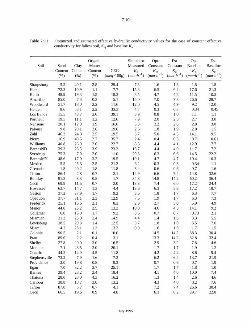
Table 7.9.1. Optimized and estimated effective hydraulic conductivity values for the case of constant effectiveconductivity for fallow soil, Kef and baseline Kb.

iiiiiiiiiiiiiiiiiiiiiiiiiiiiiiiiiiiiiiiiiiiiiiiiiiiiiiiiiiiiiiiiiiiiiiiiiiiiiiiiiiiiiiiiiiiiii

Organic Simulator Opt. Est. Opt. Est.Soil Sand Clay Matter Measured Constant Constant Baseline Baseline

Content Content Content CEC Ke Kef Kef Kb Kb

(%) (%) (%) (meq /100g) (mm .h −1) (mm .h −1) (mm .h −1) (mm .h −1) (mm .h −1)iiiiiiiiiiiiiiiiiiiiiiiiiiiiiiiiiiiiiiiiiiiiiiiiiiiiiiiiiiiiiiiiiiiiiiiiiiiiiiiiiiiiiiiiiiiiii

Sharpsburg 5.2 40.1 2.8 29.4 7.3 1.6 1.8 1.8 1.8Hersh 72.3 10.9 1.1 7.7 15.8 6.5 6.4 17.6 21.3Keith 48.9 19.3 1.5 18.3 3.5 4.7 4.8 11.5 10.5Amarillo 85.0 7.3 0.3 5.1 15.0 7.0 7.3 26.6 28.7Woodward 51.7 13.0 2.2 11.6 12.0 4.5 4.9 9.2 12.0Heiden 8.6 53.1 2.2 33.3 4.7 0.3 0.3 0.34 0.45Los Banos 15.5 43.7 2.0 39.1 3.9 0.8 1.0 1.1 1.1Portneuf 19.5 11.1 1.2 12.6 7.9 2.0 2.5 2.7 3.0Nansene 20.1 12.8 1.9 16.6 5.3 2.2 2.6 2.8 3.0Palouse 9.8 20.1 2.6 19.6 2.6 1.8 1.9 2.0 1.5Zahl 46.3 24.0 2.5 19.5 5.7 5.0 4.5 14.1 9.5Pierre 16.9 49.5 2.7 35.7 2.4 0.4 0.3 0.71 0.61Williams 40.8 26.9 2.6 22.7 8.3 4.4 4.1 12.9 7.7BarnesND 39.3 26.5 3.9 23.2 16.7 4.4 4.0 11.7 7.2Sverdrup 75.3 7.9 2.0 11.0 20.3 6.3 6.6 14.5 22.2BarnesMN 48.6 17.0 3.2 19.5 19.1 4.7 4.7 10.4 10.3Mexico 5.5 25.3 2.5 21.3 6.2 0.3 0.3 0.34 1.1Grenada 1.8 20.2 1.8 11.8 3.4 0.6 0.6 0.7 1.6Tifton 86.4 2.8 0.7 2.1 14.9 6.6 7.4 14.8 32.6Bonifay 91.2 3.3 0.5 1.7 34.8 14.8 14.2 60.2 36.4Cecil 69.9 11.5 0.7 2.0 13.3 7.4 6.0 17.2 24.4Hiwassee 63.7 14.7 1.3 4.4 13.6 6.3 5.8 17.2 18.7Gaston 37.2 37.9 1.7 9.2 3.6 1.8 1.7 6.3 7.7Opequon 37.7 31.1 2.3 12.9 7.6 1.9 1.7 6.3 7.3Frederick 25.1 16.6 2.1 8.2 2.9 2.7 3.0 5.9 4.9Manor 44.0 25.2 2.5 13.2 10.0 4.6 4.3 14.1 9.2Collamer 6.0 15.0 1.7 9.2 3.6 0.7 0.7 0.73 2.1Miamian 31.3 25.9 2.4 14.9 4.4 1.4 1.5 3.3 5.5Lewisburg 38.5 29.3 1.4 12.5 3.7 1.8 1.8 5.5 7.6Miami 4.2 23.1 1.3 13.3 0.9 1.6 1.5 1.7 1.5Colonie 90.5 2.1 0.1 10.0 14.5 14.2 38.3 30.4Pratt 89.0 2.2 0.4 3.1 13.3 14.2 32.8 32.4Shelby 27.8 29.0 3.0 16.5 2.9 3.2 7.8 4.6Monona 7.1 23.5 2.0 20.1 1.7 1.7 1.9 1.2Ontario 44.2 14.9 4.5 11.8 4.2 4.4 8.6 9.4Stephensville 73.2 7.9 1.6 7.2 6.2 6.4 13.7 21.9Providence 2.0 19.8 0.8 9.3 0.7 0.6 0.7 1.9Egan 7.0 32.2 3.7 25.1 1.7 1.7 1.8 1.0Barnes 39.4 23.2 3.4 18.4 4.1 4.0 10.0 7.4Thatuna 28.0 23.0 4.3 16.2 1.3 1.4 2.6 4.6Caribou 38.8 13.7 3.8 13.2 4.3 4.0 8.2 7.6Tifton 87.0 5.7 0.7 4.1 7.2 7.4 26.6 30.4Cecil 66.5 19.6 0.9 4.8 6.3 6.2 29.7 22.8iiiiiiiiiiiiiiiiiiiiiiiiiiiiiiiiiiiiiiiiiiiiiiiiiiiiiiiiiiiiiiiiiiiiiiiiiiiiiiiiiiiiiiiiiiiiii

July 1995

7.11

Table 7.9.2. WEPP estimated runoff in terms of: A) model efficiency on a storm-by-storm basis and B)average annual runoff.

A. Comparison of model efficiencyiiiiiiiiiiiiiiiiiiiiiiiiiiiiiiiiiiiiiiiiiiiiiiiiiiiiiiiiiiiiiiiiiiiiiiiiiiiiiiiiiiiii

Site Number Number Model Efficiencyof Years of Events WEPP WEPP

Opt. Kb CN Est. Kbiiiiiiiiiiiiiiiiiiiiiiiiiiiiiiiiiiiiiiiiiiiiiiiiiiiiiiiiiiiiiiiiiiiiiiiiiiiiiiiiiiiii

Bethany, MO 10 109 0.82 0.72 0.81Castana, IA 12 90 0.48 0.10 0.12Geneva, NY 10 97 0.73 0.58 0.62Guthrie, OK 15 170 0.86 0.77 0.85Holly Springs, MS 8 208 0.87 0.79 0.69Madison, SD 10 60 0.77 0.69 0.74Morris, MN 11 72 0.59 -1.06 -0.21Pendleton, OR 11 82 0.06 -0.33 -0.69Presque Isle, ME 9 99 0.45 -0.25 0.32Tifton, GA 7 64 0.67 0.24 0.59Watkinsville, GA 6 110 0.84 0.74 0.84iiiiiiiiiiiiiiiiiiiiiiiiiiiiiiiiiiiiiiiiiiiiiiiiiiiiiiiiiiiiiiiiiiiiiiiiiiiiiiiiiiiii

B. Comparison of average annual runoffiiiiiiiiiiiiiiiiiiiiiiiiiiiiiiiiiiiiiiiiiiiiiiiiiiiiiiiiiiiiiiiiiiiiiiiiiiiiiiiiiiiii

Site Number Average Annual Average Annual Runoffof Years Rainfall Measured CN WEPPiiiiiiiiiiiiiiiiiiiiiiiiiiiiiiiiiiiiiiiiiiiiiiiiiiiiiiiiiiiiiiiiiiiiiiiiiiiiiiiiiiiii

mm --------------------mm---------------------iiiiiiiiiiiiiiiiiiiiiiiiiiiiiiiiiiiiiiiiiiiiiiiiiiiiiiiiiiiiiiiiiiiiiiiiiiiiiiiiiiiiiBethany, MO 10 754 222 175 205Castana, IA 12 747 102* 125 148Geneva, NY 10 828 168* 79 110Guthrie, OK 15 745 154 78 121Holly Springs, MS 8 1328 557 216 299Madison, SD 10 577 56* 69 65Morris, MN 11 604 40* 33 75Pendleton, OR** 11 595 71 60 27Presque Isle, ME 9 846 107* 89 47Tifton, GA 7 1227 289 135 171Watkinsville, GA 6 1445 431 395 392iiiiiiiiiiiiiiiiiiiiiiiiiiiiiiiiiiiiiiiiiiiiiiiiiiiiiiiiiiiiiiiiiiiiiiiiiiiiiiiiiiiii

* indicates winter runoff not measured.

** Pendleton did not have any events with less than 80 mm of rainfall since last tillage.

Model efficiency is a quantification of how well the model predicted runoff on an individual stormbasis. At each of the eleven sites the model predicted runoff better on a storm-by-storm basis using theestimated Kb values (Eqs. [7.9.1] and [7.9.2]) than did the curve number approach. For purposes oferosion prediction it is more important to predict the individual storms accurately than to predict the totalannual runoff volume, because it is a relatively small number of intense storms which cause most of theerosion.

July 1995

7.12

Physically, the Kb value should approximate the value of Ke for the first storm after tillage on afallow plot of land. Figure 7.9.2 shows a plot of the optimized Kb versus a measurement of Kb obtainedusing the data from the WEPP erodibility sites under a rainfall simulator. These values are also listed inTable 7.9.2. In general, the rainfall simulator measured Kb values tended to be greater than thecorresponding optimum Kb values.

Figure 7.9.2 Baseline hydraulic conductivity values for the time-variable case measured under rainfallsimulation compared to those calibrated from curve number predictions.

7.9.2 Cropland Temporally-varying Case: Fallow Soil Adjustments to Effective Conductivity

In the natural system the hydraulic conductivity of the soil matrix is dynamically responding tochanges in the surrounding environment. Therefore, to improve the accuracy of infiltration estimatesobtained from the Green-Ampt equation in continuous simulation models, reliable estimates of thehydraulic conductivity during each event are necessary. This requires not only an appropriate inputvalue, but also a method for adjusting the hydraulic conductivity to account for temporal changes in thephysical condition of the soil. The method which is used to adjust the effective hydraulic conductivityparameter in the WEPP model was based on the results of a study which used over 220 plot years ofnatural runoff plot data from 11 different locations. By optimizing the effective Green-Ampt hydraulicconductivity for each event within a simulation, a method of determining the temporal variability in thehydraulic conductivity function was established (Risse, 1994). After a detailed statistical analysis ofseveral different WEPP parameters and functions, the following equation was selected to account for theeffects of soil crusting and tillage on the effective hydraulic conductivity:

Kbare = Kb[ CF + (1 − CF) e−C Ea (1 − RRt/0.04)][7.9.3]

where Kbare and Kb are the effective conductivity for any given event and the baseline hydraulicconductivity (mm.h −1), CF is the crust factor which ranges from 0.20 to 1.0, C is the soil stability factor(m2.J−1), Ea is the cumulative kinetic energy of the rainfall since the last tillage operation (J .m−2), and

July 1995

7.13

RRt is the random roughness of the soil surface (m). This equation has a similar form to the relationshipswhich have been proposed by Van Doren and Allmaras (1978), Eigel and Moore (1983), and Brakensiekand Rawls (1983). By selecting this form for the equation, it was assumed that the value of Kb willrepresent a freshly-tilled or maximum hydraulic conductivity which will decrease exponentially at a rateproportional to the kinetic energy of the rainfall since last tillage as it approaches the fully-crusted or finalvalue. While this form is consistent with those in the literature, most of those have been used to calculatethe hydraulic conductivity at some time within a given event rather than for a series of successive events.Generally, the energy associated with the rainfall rather than the amount is thought to control the rate atwhich the surface seal forms. The random roughness term is important, as crusts rarely form on surfaceswith random roughness greater than 4 cm and the reduction of effective hydraulic conductivity due to thecrust will generally be more significant on smoother surfaces (Rawls et al., 1990).

The crust factor, CF, provides a means of estimating the final or fully-crusted hydraulicconductivity based on the baseline values. The fully-crusted hydraulic conductivity is simply the baselinevalue multiplied by the crust factor. A relationship developed by Rawls et al. (1990) which states:

CF =IJL1 +

100 LΨhhhhhh

MJO

SChhhhhhhhhhhh[7.9.4]

where SC is the correction factor for partial saturation of the subcrust soil, Ψ is the steady state capillarypotential at the crust/subcrust interface, and L is the wetted depth (m). They also derive the followingcontinuous relationships for SC and Ψ:

SC = 0.736 + 0.19 sand [7.9.5]

Ψ = 45.19 − 46.68 SC [7.9.6]

The depth to the wetting front is calculated in the WEPP model as:

L = 0.147 − 0.15 (sand)2 − 0.0003 (clay) ρb[7.9.7]

where ρb is the bulk density (kg .m−3). If the calculated value of L is less than the crust thickness (0.005m in WEPP) then it is set equal to the crust thickness. Rawls et al. (1990) used data from 36 covered anduncovered plots to validate the fact that this method could provide reasonable estimates of crustedhydraulic conductivities based on freshly-tilled hydraulic conductivities. Table 7.9.3 compares the crustfactor calculated using these equations to two values of maximum adjustment taken from the naturalrunoff plot data.

At six of the ten sites, the calculated crust factor was within 10% of the maximum adjustmentcalculated from the data. At Bethany and Castana, the reduction in hydraulic conductivity was not assignificant as that predicted by the crust factor, while the data from Holly Springs indicated that the crustfactor should have been slightly higher. The data indicated that the crust factor calculated by theequations of Rawls et al. (1990) can adequately predict the maximum reduction in conductivity due tocrust formation.

July 1995

7.14

Table 7.9.3. Comparison of optimized and calculated values for the crust factors and soil stabilityconstants.

iiiiiiiiiiiiiiiiiiiiiiiiiiiiiiiiiiiiiiiiiiiiiiiiiiiiiiiiiiiiiiiiiiiiiiiiiiiiiiiiiiiiii

Site Avg. Ke for Avg. Ke for 10 CF calc. CF optimum CF from Optimum Calculatedevents w/ events w/ max. from Kf/Kb from SAS Rawls et al. C Crfcum<1.0 rfcum (1990) (m2.J−1) (m2.J−1)iiiiiiiiiiiiiiiiiiiiiiiiiiiiiiiiiiiiiiiiiiiiiiiiiiiiiiiiiiiiiiiiiiiiiiiiiiiiiiiiiiiiii

Bethany 1.72 0.61 0.35 0.77 0.20 0.0001 0.0051Castana 1.87 1.18 0.63 0.63 0.27 0.0002 0.0001Geneva 4.35 1.85 0.42 0.27 0.37 0.0020 0.0041Holly Springs 1.40 0.11 0.08 0.27 0.29 0.0009 0.0036Madison 3.84 0.70 0.18 0.33 0.20 0.0007 0.0001Morris 11.57 2.11 0.18 0.23 0.27 0.0034 0.0033Pendleton * 0.45 * 0.14 0.28 0.0015 0.0026Presque Isle 4.13 1.18 0.28 0.16 0.38 0.0033 0.0014Tifton 13.18 2.16 0.20 0.20 0.20 0.0118 0.0122Watkinsville 8.13 2.73 0.20 0.55 0.20 0.0312 0.0295iiiiiiiiiiiiiiiiiiiiiiiiiiiiiiiiiiiiiiiiiiiiiiiiiiiiiiiiiiiiiiiiiiiiiiiiiiiiiiiiiiiiii

* Pendleton did not have any events with less than 80 mm of rainfall since last tillage.

The soil stability factor, C, represents the rapidity that the effective conductivity declines from Kbto its fully-crusted value. The values obtained by fitting Eq. [7.9.3] to the optimized effectiveconductivities for the natural runoff plot data ranged from 0.00006 to 0.0312 m2.J−1. This generallyagreed with the range of values reported in the literature (0.00012-0.0356). For this equation to be widelyapplicable, the user must have a method for obtaining accurate values of C since few measured values arereadily available. Regression analysis between the C values given in Table 7.9.3 and soil propertiesindicated that the primary soil factors influencing the rate of surface seal development were sand content(r=0.68), bulk density (r=0.66), and silt content (r=-0.72). Bosch and Onstad (1988) had similar findingsin a study they conducted. Based on these findings, the following equation was developed to estimate thesoil stability factor based on soil properties:

C = −0.0028 + 0.0113 sand+ 0.125IJL CEC

clayhhhhhMJO

[7.9.8]

where CEC is the cation exchange capacity (meq /100g). Bounds of 0.0001<C<0.010 were imposed onthis equation to prevent negative C values on soils with very low sand and clay contents. Using thisequation, soils with high amounts of sand or clay and a low CEC will be predicted to form crust morerapidly. Eq. [7.9.8] provided estimates of C which were within one order of magnitude of the optimizedvalues for eight of the ten sites (Table 7.9.3).

Figure 7.9.3 shows the optimized event conductivities plotted against those calculated using thetillage adjustment with an optimized baseline hydraulic conductivity for soils with a high, medium, andlow value of C. In these figures, it is evident that the tillage adjustment using the estimated C values isaccurately predicting the trend of a reduction in Ke with increasing rainfall kinetic energy since lasttillage, however, this adjustment does not account for most of the variability in the Kopt values.

July 1995

7.15

CalculatedOptimizedCumulative Rainfall KE (J/ m

2)

C=0.012

C=0.005

C=0.0001

Tifton

Geneva

Castana

Ke/Kb

0.0

0.5

1.0

1.5

2.0

2.5

3.0

0 2000 4000 6000 8000 10000

0.0

0.5

1.0

1.5

2.0

2.5

3.0

0 2000 4000 6000 8000 10000

0.0

0.5

1.0

1.5

2.0

2.5

3.0

0 2000 4000 6000 8000 10000

Figure 7.9.3. Comparison of optimized effective conductivities to effective conductivities predicted bythe proposed tillage adjustments at three sites.

To compare the effects of using each of these adjustments on predicted runoff amounts, eachadjustment was incorporated into WEPP. Two different developmental WEPP versions were tested; 1) aconstant Kec version in which no temporal variation was allowed; and 2) a version which included thetillage and crusting adjustments. Both versions were run using calibrated values of hydraulicconductivity. The optimized baseline conductivities and model efficiencies of each of the versions isgiven in Table 7.9.4.

The baseline values of hydraulic conductivity were all higher than the effective conductivitiesobtained for the constant value version. This was expected since the constant values represent the

July 1995

7.16

average effective conditions rather than the freshly-tilled conditions. Using the tillage adjustment theaverage effective value, Kec was approximately 42% of Kb . The average model efficiency was higher forthe version of the model which used the tillage adjustment and this version performed the better at nine ofthe eleven sites. The correlation coefficients, r 2, were generally close to the model efficiencies andindicated the same trends. The slope and intercept of the regression line between measured and predictedvalues can be used as a measure of bias.

Table 7.9.4. Comparison of optimized baseline conductivities and model results for WEPP usingconstant values of hydraulic conductivity and temporally varying values.

iiiiiiiiiiiiiiiiiiiiiiiiiiiiiiiiiiiiiiiiiiiiiiiiiiiiiiiiiiiiiiiiiiiiiiiiiiiiiiiiiiiii

Constant Kec (mm.h −1) Kb (mm.h −1) with tillageand crusting adjustment

Site Kec ME* Slp. Int. r 2 Kb ME Slp Int r 2iiiiiiiiiiiiiiiiiiiiiiiiiiiiiiiiiiiiiiiiiiiiiiiiiiiiiiiiiiiiiiiiiiiiiiiiiiiiiiiiiiiii

Bethany 1.22 0.81 0.90 0.02 0.81 3.65 0.82 0.91 0.81 0.82Castana 2.04 0.46 0.82 0.50 0.59 2.38 0.49 0.84 0.05 0.62Geneva 2.27 0.63 0.83 0.67 0.67 5.14 0.72 0.80 0.32 0.74Guthrie 6.19 0.85 0.97 -0.99 0.87 16.73 0.85 0.97 -1.04 0.87Holly Springs 0.31 0.84 0.87 1.39 0.84 0.72 0.87 0.85 1.82 0.87Madison 1.80 0.74 0.69 1.57 0.75 2.01 0.77 0.71 1.42 0.78Morris 7.68 0.40 0.69 0.05 0.52 16.41 0.59 0.74 -0.29 0.66Pendleton 0.51 0.07 0.61 -0.18 0.41 1.76 0.07 0.67 -0.12 0.41Presque Isle 2.38 0.19 0.55 1.12 0.36 3.82 0.46 0.63 0.68 0.53Tifton 7.87 0.49 0.79 0.77 0.59 18.14 0.66 0.85 2.19 0.69Watkinsville 4.41 0.84 0.97 -0.81 0.86 19.15 0.84 1.01 -1.13 0.87Average 0.56 0.79 0.37 0.66 0.65 0.82 0.43 0.71iiiiiiiiiiiiiiiiiiiiiiiiiiiiiiiiiiiiiiiiiiiiiiiiiiiiiiiiiiiiiiiiiiiiiiiiiiiiiiiiiiiii

* Model efficiency calculated between WEPP predicted runoff and measured values. Regression statistics calculated between

measured and predicted runoff.

The results from a perfect model would have a slope of one and a intercept of zero. For bothversions of the model and almost every site, the slopes were less than one and the intercepts were greaterthan zero. This indicates that both of the versions were over-predicting runoff for the smaller events andunder-predicting runoff for the larger events. The version with the tillage adjustment appeared to be lessbiased as it had a higher slope.

7.9.3 Cropland Temporally-Varying Case: Cropping Adjustments to Effective Conductivity

7.9.3.1 Temporal Adjustment for Row Crops

Surface cover is known to be effective in reducing soil crusting and increasing effective hydraulicconductivity (Ke). Flow through macropores formed by root and soil fauna under cropped conditionsplays an important role in increasing Ke. As compared to the corresponding fallow conditions, the degreeof the increase under cropped conditions heavily depends on crop and residue management practices,tillage systems, soil properties, and rainfall characteristics, as well as their interactions. Wischmeier(1966) observed that water infiltration was more a characteristic of surface conditions and managementthan of a specific soil type, and that infiltration increased with larger storms. This indicates that theeffects of these variables and their interactions must be considered in order to successfully apply theGreen-Ampt equation to cropped conditions.

July 1995

7.17

A total of 328 plot-years of data from natural runoff plots on 8 sites with 1912 measured runoffvalues were used to develop equations for adjusting Ke for row cropped conditions (Table 7.9.5). Themanagement input files were compiled based on recorded data. Plant growth parameters were calibratedto obtain realistic above-ground biomass. Soil, slope, and climate input files were prepared usingmeasured data. Events which accounted for about 60-70% of the total annual runoff were strictly selectedfrom each site based on data quality.

Table 7.9.5. Site and crop management descriptions.iiiiiiiiiiiiiiiiiiiiiiiiiiiiiiiiiiiiiiiiiiiiiiiiiiiiiiiiiiiiiiiiiiiiiiiiiiiiiiiiiiiiii

Number of Number ofSite Crop management reps Years eventsiiiiiiiiiiiiiiiiiiiiiiiiiiiiiiiiiiiiiiiiiiiiiiiiiiiiiiiiiiiiiiiiiiiiiiiiiiiiiiiiiiiiii

Holly Springs,MS a. fallow 2 1961-68 208slope: 0.05 m/m b. cont. corn, sprint TP† 2 1961-68 163size: 4x22.3 m

Madison,SD a. fallow 3 1962-70 59slope: 0.06 m/m b. cont. corn, spring TP 3 1962-70 48size:4x22.3 m c. cont. corn, no TP 3 1962-70 50

d. cont. oats 3 1962-64 15

Morris, MN a. fallow 3 1962-71 67slope:0.06 m/m b. cont. corn, fall TP 3 1962-71 67size:4x22.3 m

Presque Isle, ME a. fallow 3 1961-65 65slope: 0.08 m/m b. cont. potato 3 1961-65 64size: 3.7x22.3 m

Watkinsville, GA a. fallow 2 1961-67 147slope: 0.07 m/m b. cont. corn, spring TP 2 1961-67 97size: 4x22.3 m c. cont. cotton, spring TP 2 1961-67 112

Bethany, MO a. fallow 1 1931-40 109slope: 0.07 m/m b. cont. corn, spring TP 1 1931-40 112size: 4.3x22.3 m

Geneva, NY a. fallow 1 1937-46 97slope: 0.08 m/m b. summer fallow, winter rye 1 1937-46 77size: 1.8x22.3 m c. cont. soybean, spring TP 1 1937-46 45

Guthrie, OK a. fallow 1 1942-56 170slope: 0.08 m/m b. cont. cotton, spring TP 1 1942-56 140size: 1.8x22.3 miiiiiiiiiiiiiiiiiiiiiiiiiiiiiiiiiiiiiiiiiiiiiiiiiiiiiiiiiiiiiiiiiiiiiiiiiiiiiiiiiiiiii

† TP, turn plow

July 1995

7.18

Canopy height has a significant effect on surface runoff (Khan et al., 1988). Based on the measuredfall velocities for a raindrop size (diameter) of 2.5 mm at various fall heights (Laws, 1941), the followingcorrection factor (Ch) for canopy height effectiveness as cover relative to infiltration was developed

Ch = e

IJL−0.33

2hhh

MJO r 2 = 0.99

[7.9.9]

where h is the fall height in meters. Average fall height was calculated as one half of the crop height inWEPP. With Eq. [7.9.9], the effective canopy cover (ccovef) can be computed by

ccovef = cancov Ch[7.9.10]

where cancov is the canopy cover (0-1).

The total effective surface cover (scovef) can be computed by

scovef = ccovef + rescov − (ccovef ) (rescov) [7.9.11]

where rescov is the residue cover (0-1).

Correlation coefficients of selected variables to optimized Ke for each site are tabulated in Table7.9.6. For cover-related variables, the correlation coefficients from the pooled data increased in the orderof: cancov, ccovef, rescov, and scovef. This sequence implies that 1). The adjustment of canopy cover byEq. [7.9.10] is useful; 2). Residue cover is more correlated to Ke than canopy cover; 3). The combinedeffects of the two are greater than either one of them when used alone. The rainfall amount (rain) showeda very strong correlation with Ke. This behavior could be explained by macropore flow phenomena.More importantly, the product of rain and scovef exhibited a better overall correlation coefficient thaneither rain or scovef, indicating a positive interaction between the two. Thus, this interactive productshould be a better predictor for Ke.

Table 7.9.6. Correlation coefficients of selected variables to optimized event hydraulic conductivities.iiiiiiiiiiiiiiiiiiiiiiiiiiiiiiiiiiiiiiiiiiiiiiiiiiiiiiiiiiiiiiiiiiiiiiiiiiiiiiiiiiiiii

TotalEffective effective Residue Days

Canopy canopy Residue surface mass Buried Total since Rainfall Rainfallcover cover cover cover on residue root last amount &cover

Site (cancov) (ccovef) (rescov) (scovef) ground mass mass tillage (rain) term†iiiiiiiiiiiiiiiiiiiiiiiiiiiiiiiiiiiiiiiiiiiiiiiiiiiiiiiiiiiiiiiiiiiiiiiiiiiiiiiiiiiiiiHolly Springs .11 .11 .26 .27 .24 .17 .31 .20 .31 .41Madison .20 .19 .03‡ .17 .07‡ .08‡ .17 -.01‡ .28 .32Morris .04‡ .05‡ -.02‡ .05‡ -.01‡ -.04‡ .04‡ -.15‡ .68 .20Presque Isle -.04‡ -.04‡ -.16‡ -.08‡ .00‡ .04‡ .01‡ -.05‡ .33 .06Watkinsville .18 .19 .20 .31 .18 .28 .31 .05‡ .40 .49Bethany .16 .17 -.10‡ .14 -.09‡ .12‡ .06‡ .00‡ .27 .22Geneva .43 .42 .27 .49 .28 .37 .49 .08‡ .64 .82Guthrie .14 .15 .06‡ .16 .05‡ .30 .27 -.18 .42 .28iiiiiiiiiiiiiiiiiiiiiiiiiiiiiiiiiiiiiiiiiiiiiiiiiiiiiiiiiiiiiiiiiiiiiiiiiiiiiiiiiiiiiipooled* .10 .12 .13 .20 .14 .17 .06 .11 .38 .39iiiiiiiiiiiiiiiiiiiiiiiiiiiiiiiiiiiiiiiiiiiiiiiiiiiiiiiiiiiiiiiiiiiiiiiiiiiiiiiiiiiiii

† Rain*scovef‡ Not significant at 5% level.

* Using the lumped database from all the sites.

July 1995

7.19

Based on the above analyses, the final model structure was proposed as:

Ke = Kbare (1 − scovef) + (c rain scovef) [7.9.12]

where Kbare is the Ke of the bare area (mm.h −1) and can be estimated by Eq. [7.9.3], c is a regressioncoefficient and was estimated for each soil series at each site, and rain is the storm rainfall amount inmillimeters. This equation assumes that Ke for any given area can be conceptualized as the areally-weighted average of Kbare and Ke in the covered area. The latter, being closely related to the variable ofrain*scovef, can be well represented by this variable. This model formulation attempts to reflect thegeneral conditions. For the fallow case, Eq. [7.9.12] reduces to Ke = Kbare . While under the fully-covered conditions, the effect of soil crusting is neglected and Ke is adjusted for the effects of surfacecover and rainfall amount. The c values were strongly related to basic soil properties such as sand andclay content, and to Kb which is estimated from basic soil properties (Eqs. [7.9.1] and [7.9.2]). Therelationship to Kb can be described by :

c = 0.0534 + 0.01179 (Kb) [7.9.13]

where Kb is in mm.h −1. Substituting the above equation for c, the final adjustment equation becomes:

Ke = Kbare (1 − scovef) + (0.0534 + 0.01179 Kb) (rain) (scovef ) [7.9.14]

The predicted mean Ke and total WEPP predicted runoff using Eq. [7.9.14], along with measuredvalues, are presented in Table 7.9.7. The predicted mean Ke agreed well with the optimized mean Ke.The total measured runoff of the selected events and the total predicted runoff matched well with r 2 andslope of regression being 0.94 and 0.99, respectively. The model efficiency, calculated on an event basis,averaged 0.64, which indicates that Eq. [7.9.14] works better than just using a constant mean for Ke.

This can also be clearly seen in Fig. 7.9.4. In addition, the seasonal variation of Ke and runoff werealso represented by the equation.

July 1995

7.20

Table 7.9.7. Total rainfall, optimized and predicted effective conductivity (Ke), and measured andpredicted total runoff for the selected events.

iiiiiiiiiiiiiiiiiiiiiiiiiiiiiiiiiiiiiiiiiiiiiiiiiiiiiiiiiiiiiiiiiiiiiiiiiiiiiiiiiiiii

Ke† Total runoff ModelTotal hhhhhhhhhhhhhhhhhhh hhhhhhhhhhhhhhhhhh efficiency‡

Site Management rainfall Optimized Predicted Measured Predicted (ME)iiiiiiiiiiiiiiiiiiiiiiiiiiiiiiiiiiiiiiiiiiiiiiiiiiiiiiiiiiiiiiiiiiiiiiiiiiiiiiiiiiiii

mm -------mm.h −1------- -------mm-------iiiiiiiiiiiiiiiiiiiiiiiiiiiiiiiiiiiiiiiiiiiiiiiiiiiiiiiiiiiiiiiiiiiiiiiiiiiiiiiiiiiii

Holly Springs fallow 5742 0.53corn 5049 1.34 1.20 1793 2014 .582

Madison fallow 1553 1.54corn TP 1310 1.83 1.62 322 311 .783corn No TP 1359 1.76 1.75 311 275 .747oats 410 1.86 1.76 86 88 .775

Morris fallow 1985 5.85corn 1987 6.11 6.74 319 310 .340

Presque Isle fallow 1321 1.53potato 1296 1.57 2.75 432 231 .291

Watkinsville fallow 4277 3.34corn 3566 8.45 9.66 675 793 .823cotton 3846 7.36 8.65 834 911 .791

Bethany fallow 3330 1.42corn 3375 1.73 1.60 1375 1308 .845

Geneva fallow 2292 2.40winter rye 1912 3.95 2.91 375 534 .511soybean 1446 8.70 3.66 51 338 **

Guthrie fallow 5313 5.58cotton 4820 8.16 8.87 1239 1204 .793iiiiiiiiiiiiiiiiiiiiiiiiiiiiiiiiiiiiiiiiiiiiiiiiiiiiiiiiiiiiiiiiiiiiiiiiiiiiiiiiiiiii

† Means of all selected events calculated on an event basis.‡ Calculation on an event basis.

** Indicates negative model efficiency.

July 1995

7.21

Figure 7.9.4. Measured vs. predicted runoff for each individual storm on selected sites under row cropconditions.

July 1995

7.22

7.9.3.2 Temporal Adjustment for Perennial Crops

The sites used for row crop adjustment were also used for perennial crops except for the Madisonsite where perennial crops were not grown (Table 7.9.8). Therefore, the same climate, slope, and soilinput files were used. The management input files were prepared according to the recorded data, and theplant growth parameters were calibrated. Two common cropping systems, continuous meadow androtation meadow, were included. A total of 88 plot-years of data with 506 measured runoff values wereused for the validation.

Table 7.9.8. Background information of the database used for Ke adjustment under perennial crops.iiiiiiiiiiiiiiiiiiiiiiiiiiiiiiiiiiiiiiiiiiiiiiiiiiiiiiiiiiiiiiiiiiiiiiiiiiiiiiiiiiiiii

NumberNumber of Periods Years in of events

Site Crop Management reps used meadow usediiiiiiiiiiiiiiiiiiiiiiiiiiiiiiiiiiiiiiiiiiiiiiiiiiiiiiiiiiiiiiiiiiiiiiiiiiiiiiiiiiiiii

Holly Springs, MS meadow-corn-meadow 2 1962-68 5 101

Morris, MN meadow-corn-oats 3 1962-71 4 18

Presque Isle, ME potato-oats-meadow 3 1961-65 1 4

Watkinsville, GA corn-meadow-meadow 2 1961-67 4 44

Bethany, MO cont. alfalfa 1 1931-40 10 83cont. blue grass 1 1931-40 10 79

Geneva, NY cont. red clover 1 1937-41 5 19cont. blue grass 1 1937-46 10 30

Guthrie, OK cont. blue grass 1 1942-56 15 96wheat-meadow-cotton 1 1942-56 5 32iiiiiiiiiiiiiiiiiiiiiiiiiiiiiiiiiiiiiiiiiiiiiiiiiiiiiiiiiiiiiiiiiiiiiiiiiiiiiiiiiiiiii

Since similar correlation relationships between the selected variables and optimized Ke valuesexisted for both row crops and perennial crops, Eq. [7.9.2] was used to generate the first approximation ofeffective hydraulic conductivity (Kappr) for each event under meadow conditions. The mean optimizedKe and mean generated Kappr on the 7 sites were used to develop the following adjustment equation

Ke = 1.81 (Kappr) [7.9.15]

where Kappr is in mm.h −1 and can be replaced by Eq. [7.9.14].

Ke = 1.81 (Kbare (1 − scovef) + (0.0534 + 0.01179 Kb) (rain) (scovef ) [7.9.16]

This final adjustment equation shows that with identical effective surface cover (scovef) the Ke ofperennial crops is approximately 1.8 times higher than that from the corresponding row croppedconditions. This is due to the fact that perennial crops, often accompanied by the formation of a thicklayer of organic matter or plant residue on soil surface, are more effective in improving soil aggregation,controlling soil crusting, and forming and preserving bio-pores.

As is shown in Table 7.9.9, the optimized Ke and predicted Ke matched well. The coefficient ofdetermination for predicted mean Ke versus the optimized values was 0.90 and slope of regression was0.96. The total runoff from the selected events was also predicted well. The r 2 and slope of regressionwere 0.94 and 0.99, respectively. Model efficiency, calculated on an event basis, averaged 0.49 (Table

July 1995

7.23

7.9.9), indicating the individual storm runoff was predicted reasonably well. The predicted and measuredannual runoff was plotted in Fig. 7.9.5. Linear regression fit the data well (r 2=0.76) with little bias(slope=0.88).

Figure 7.9.5. Measured vs. predicted annual runoff for the data used under meadow conditions.

Table 7.9.9. Total rainfall, optimized and predicted effective conductivity (Ke), and measured andpredicted total runoff for the events selected in the years when meadow was grown.

iiiiiiiiiiiiiiiiiiiiiiiiiiiiiiiiiiiiiiiiiiiiiiiiiiiiiiiiiiiiiiiiiiiiiiiiiiiiiiiiiiiii

Crop Total Ke† Total runoff ModelSite Management Rainfall Optimized Predicted Measured Predicted Efficiency

(mm) (mm.h −1) (mm.h −1) (mm) (mm) (ME)‡iiiiiiiiiiiiiiiiiiiiiiiiiiiiiiiiiiiiiiiiiiiiiiiiiiiiiiiiiiiiiiiiiiiiiiiiiiiiiiiiiiiii

Holly Springs bermuda-corn-bermuda 3497 1.62 2.49 1196 1256 .675Morris grass-corn-oats 646 12.15 17.55 27 17 .649Watkinsville corn-bermuda-bermuda 1682 11.87 13.36 154 269 .573Bethany cont. alfalfa 2900 6.40 4.98 310 553 .290

cont. brome grass 2761 5.47 5.90 308 265 .466Geneva cont. red clover 549 6.71 6.54 35 54 --

cont. brome grass 1131 10.23 7.97 3 93 --Guthrie cont bermuda grass 3767 19.55 20.30 189 373 .734

wheat-clover-cotton 1270 13.81 22.19 112 145 .275iiiiiiiiiiiiiiiiiiiiiiiiiiiiiiiiiiiiiiiiiiiiiiiiiiiiiiiiiiiiiiiiiiiiiiiiiiiiiiiiiiiii

† Means of all selected events.

‡ Calculated on an event basis, and negative ME is not presented.

July 1995

7.24

7.9.4 Cropland Time-Invariant Effective Hydraulic Conductivity Values

For the case of time-invariant effective conductivity, the input value of Ke must represent both thesoil type and the management practice. This method is corollary to the curve number approach forpredicting runoff, and in fact, the estimation procedures discussed here were derived using curve numberoptimizations, so the runoff volumes predicted should correspond closely to curve number predictions.One difference between this method and the curve number method is that no soil moisture correction isnecessary, since WEPP takes into account moisture differences via internal adjustments to the wettingfront matric potential term of the Green-Ampt equation.

Figure 7.9.6. Optimized effective conductivity values for fallow soil conditions, Kef , plotted versus sandcontent of the soil. This is for the case of time-invariant conductivity.

The estimation procedure involves two steps. In step one a fallow soil Kef is calculated. In step 2the fallow soil Kef is adjusted based on management practice using a runoff ratio to obtain the input valueof Kec.

Step 1: Kef was found to be related to the amount of sand in the upper 20 cm of the soil profile (Fig.7.9.6). Thus, one may use the hydrologic soil group and sand content to estimate Kef (mm.h −1):

Hydrologic Soil Group FormulaA Kef = 14.2B Kef = 1.17 + 7.2(sand)C Kef = 0.50 + 3.2(sand)D Kef = 0.34

July 1995

7.25

Step 2: Multiply Kef by the value in the table below to obtain Ke (mm.h −1):

Hydrologic Soil GroupA B,C Diiiiiiiiiiiiiiiiiiiiiiiiiiiiiiiiiiiiiiiiiiii

Fallow 1.00 1.00 1.00Conv. Tillage - Corn 1.35 1.58 1.73Conv. Tillage - Soybeans 1.39 1.70 2.00Conserv. Till. - Corn 1.48 1.79 2.21Conserv. Till. - Soybeans 1.50 1.91 2.49Small Grain 1.84 2.14 2.48Alfalfa 2.86 3.75 6.23Pasture (Grazed) 3.66 4.34 5.96Meadow (Grass) 6.33 9.03 15.5iiiiiiiiiiiiiiiiiiiiiiiiiiiiiiiiiiiiiiiiiiii

For other cases, such as for crop rotations, ratios of Ke/Kef may be estimated from curve numbervalues using the equation:

Kec =1 + 0.051e 0.062CN

56.82 Kef0.286

hhhhhhhhhhhhhhh − 2[7.9.17]

Table 7.9.10 shows the model results as applied to data from fallow natural runoff plots. The testsindicate that this method gives a slightly better fit to the measured data than does the curve numbermethod, as evidenced by the greater event-by-event model efficiencies. Tables 7.9.11 and 7.9.12 showthe model results as applied to data from several cropped natural runoff plots. In Table 7.9.11, Eq.[7.9.17] was used to estimate Kec, whereas the ratio values listed above for the 7 management practiceswere used in Table 7.9.12. WEPP produced better model efficiencies for most of the applications thandid the curve number procedure.

Table 7.9.10. Measured runoff volumes, curve numbers and WEPP predicted runoff volumes, andmodel efficiency for the fallow runoff plot data.

iiiiiiiiiiiiiiiiiiiiiiiiiiiiiiiiiiiiiiiiiiiiiiiiiiiiiiiiiiiiiiiiiiiiiiiiiiiiiiiiiiiiiiAverage runoff per event (mm) Model efficiency

Site hhhhhhhhhhhhhhhhhhhhhhhhhhhhhhhhhhhhhhhhhhhhhhhhhhhhhhhhhhhhhhhh

Measured CN WEPP CN WEPPiiiiiiiiiiiiiiiiiiiiiiiiiiiiiiiiiiiiiiiiiiiiiiiiiiiiiiiiiiiiiiiiiiiiiiiiiiiiiiiiiiiiiiBethany, MO 14.43 10.03 10.72 0.72 0.77Castana, IA 11.47 11.87 14.41 0.10 0.11Geneva, NY 7.87 6.08 6.45 0.58 0.63Guthrie, OK 10.91 10.58 12.46 0.77 0.80Holly Springs, MS 15.17 12.62 13.58 0.79 0.84Madison, SD 7.96 6.72 9.40 0.69 0.70Morris, MN 5.55 8.77 10.94 -1.06 -1.20Pendleton, OR 3.18 1.87 1.24 -0.26 -0.08Presque Isle, ME 6.91 4.87 4.86 -0.25 0.18Tifton, GA 19.58 21.70 21.17 0.36 0.43Watkinsville, GA 13.42 11.98 13.41 0.75 0.83iiiiiiiiiiiiiiiiiiiiiiiiiiiiiiiiiiiiiiiiiiiiiiiiiiiiiiiiiiiiiiiiiiiiiiiiiiiiiiiiiiiiii

July 1995

7.26

Table 7.9.11. Measured runoff volumes, curve number and WEPP predicted runoff volumes, and modelefficiency for the cropped runoff plot data. The estimations of effective conductivity arefrom the use of Eq. [7.9.17].

iiiiiiiiiiiiiiiiiiiiiiiiiiiiiiiiiiiiiiiiiiiiiiiiiiiiiiiiiiiiiiiiiiiiiiiiiiiiiiiiiiiii

Average runoff per event (mm) Model efficiencyhhhhhhhhhhhhhhhhhhhhhhhhhhhhhhhh hhhhhhhhhhhhhhhhhh

Management Curve CurveSite Practice Measured Number WEPP Number WEPPiiiiiiiiiiiiiiiiiiiiiiiiiiiiiiiiiiiiiiiiiiiiiiiiiiiiiiiiiiiiiiiiiiiiiiiiiiiiiiiiiiiii

Bethany, MO Alfalfa 3.72 1.25 1.41 0.33 0.49Bethany, MO Blue grass 3.91 1.30 1.28 0.43 0.42Bethany, MO Corn 12.20 6.65 7.63 0.66 0.73Guthrie, OK Blue grass 1.94 2.04 4.88 0.58 0.32Guthrie, OK Cotton 8.85 9.03 14.21 0.68 0.49Holly Springs, MS Corn 11.00 11.91 12.01 0.15 0.38Madison, SD Corn 6.70 4.90 6.07 0.55 0.78Madison, SD No-till corn 6.22 3.57 4.75 0.50 0.76Watkinsville, GA Corn 6.96 9.97 14.15 0.37 0.04Watkinsville, GA Cotton 7.48 8.91 12.22 0.49 0.09iiiiiiiiiiiiiiiiiiiiiiiiiiiiiiiiiiiiiiiiiiiiiiiiiiiiiiiiiiiiiiiiiiiiiiiiiiiiiiiiiiiii

Table 7.9.12. Measured runoff volumes, curve number and WEPP predicted runoff volumes, and modelefficiency for the cropped runoff plot data. The estimations of effective conductivity arefrom the use of tabulated values in the text.

iiiiiiiiiiiiiiiiiiiiiiiiiiiiiiiiiiiiiiiiiiiiiiiiiiiiiiiiiiiiiiiiiiiiiiiiiiiiiiiiiiiii

Average runoff per event (mm) Model efficiencyhhhhhhhhhhhhhhhhhhhhhhhhhhhhhhhhh hhhhhhhhhhhhhhhhhhManagement Curve Curve

Site Practice Measured Number WEPP Number WEPPiiiiiiiiiiiiiiiiiiiiiiiiiiiiiiiiiiiiiiiiiiiiiiiiiiiiiiiiiiiiiiiiiiiiiiiiiiiiiiiiiiiii

Bethany, MO Alfalfa 3.72 1.25 1.46 0.33 0.50Bethany, MO Blue grass 3.91 1.30 1.33 0.43 0.43Bethany, MO Corn 12.20 6.65 7.55 0.66 0.72Guthrie, OK Blue grass 1.94 2.04 2.74 0.58 0.80Guthrie, OK Cotton 8.85 9.03 11.46 0.68 0.68Holly Springs, MS Corn 11.00 11.91 13.35 0.15 0.29Madison, SD Corn 6.70 4.90 7.56 0.55 0.70Madison, SD No-till corn 6.22 3.57 5.91 0.50 0.76Watkinsville, GA Corn 6.96 9.97 11.44 0.37 0.37Watkinsville, GA Cotton 7.48 8.91 10.50 0.49 0.55iiiiiiiiiiiiiiiiiiiiiiiiiiiiiiiiiiiiiiiiiiiiiiiiiiiiiiiiiiiiiiiiiiiiiiiiiiiiiiiiiiiii

7.9.5 Cropland Bio-pore Adjustments to Effective Conductivity

Accounting for infiltration differences as a function of wormholes may be made by adjusting theinput value of effective conductivity. The suggestions listed here are preliminary guidelines which arebased on interpretations of personal communications regarding the effects of bio-pores on permeabilityclasses from the SCS Soil Survey Laboratory Staff. The first step is to identify the bio-pore influenceclass from Table 7.9.13 below. Then, the input value of either Kec or Kb as calculated above should bemultiplied by the ratio shown in Table 7.9.14 below.

July 1995

7.27

Table 7.9.13. Classes of bio-pore influence defined by abundance and size classes.iiiiiiiiiiiiiiiiiiiiiiiiiiiiiiiiiiiiiiiiiiiiiiiiiiiiiiiiiiiiii

Pore Sizehhhhhhhhhhhhhhhhhhhhhhhhhhhhhhhhhhhhhhhhhhhhhhhhhh

Abundance Medium Coarse Very Coarseiiiiiiiiiiiiiiiiiiiiiiiiiiiiiiiiiiiiiiiiiiiiiiiiiiiiiiiiiiiiii

Few Small Moderate Moderately LargeCommon Moderate Moderately Large LargeMany Moderately Large Large Very Largeiiiiiiiiiiiiiiiiiiiiiiiiiiiiiiiiiiiiiiiiiiiiiiiiiiiiiiiiiiiiii

Table 7.9.14. Increase in input Kec or Kb by bio-pore influence.iiiiiiiiiiiiiiiiiiiiiiiiiiiiiiiiiiiiiiiiiiiiiiiiiiiiiiii

Input Kec,Kb Bio-pore Influence Ratio for Kec, Kb IncreaseiiiiiiiiiiiiiiiiiiiiiiiiiiiiiiiiiiiiiiiiiiiiiiiiiiiiiiiiVery Low Moderate 12<0.5 mm.h −1 Large 15

Very Large 18Low Moderate 90.5-1 mm.h −1 Large 12

Very Large 15Moderately Low Moderate 61-2 mm.h −1 Large 9

Very Large 12Moderate Moderate 32-3 mm.h −1 Large 6

Very Large 9Moderately High Moderate 23-5 mm.h −1 Large 2.5

Very Large 3iiiiiiiiiiiiiiiiiiiiiiiiiiiiiiiiiiiiiiiiiiiiiiiiiiiiiiii

July 1995

7.28

7.9.6 Rangeland Effective Hydraulic Conductivity Estimation

Baseline default equations for predicting Ke on rangelands were developed from rainfall simulationdata collected on 150 plots from 34 locations across the western United States. The data were collectedduring the WEPP rangeland field experiment and as a part of a joint Agricultural Research Service andNatural Resource Conservation Service project known as the Interagency Rangeland Water Erosion Team(IRWET). Site description information for each location is given in Tables 7.9.15 and 7.9.16. Kerange foreach of the 150 plots was obtained by optimizing the WEPP model based on total runoff volume (mm).Multiple regression procedures were then used to develop predictive equations for Kerange based on bothbiotic and abiotic plot-specific properties. The resulting equations are as follows.

If the rill surface cover (surface cover outside the plant canopy) is less than 45%, then Kerange ispredicted from:

Kerange = 57.99 − 14.05 ln (CEC) + 6.20 ln (ROOT 10) − 473.39 BASR 2 + 4.78 RESI [7.9.18]

where CEC is cation exchange capacity of the surface soil (meq /100g), ROOT 10 is root biomass in thetop 10 cm of the soil (kg .m−2), BASR is the fraction of basal surface cover in rill (outside the plantcanopy) areas based on the entire overland flow element area (0-1), and RESI is the fraction of littersurface cover in interrill (under plant canopy) areas based on the entire overland flow element area (0-1).BASR is the product of the fraction of basal surface cover in rill areas (FBASR, expressed as a fraction oftotal basal surface cover) and total basal surface cover (BASCOV). RESI is the product of the fraction oflitter surface cover in interrill areas (FRESI, expressed as a fraction of total litter surface cover) and totallitter surface cover (rescov).

If rill surface cover is greater than or equal to 45%, then Kerange is predicted from:

Kerange = −14.29 − 3.40 ln (ROOT 10) + 37.83 sand + 208.86 orgmat

+ 398.64 RR − 27.39 RESI + 64.14 BASI [7.9.19]

where sand is the fraction of sand in the soil (0-1), orgmat is the fraction of organic matter in the soil (0-1), RR is the soil surface random roughness (m), and BASI is the fraction of basal surface cover in interrillareas based on the entire overland flow element area (0-1). BASI is the product of the fraction of basalsurface cover in interrill areas (FBASI, expressed as a fraction of total basal surface cover) and total basalsurface cover (BASCOV).

The user is cautioned against using Eqs. [7.9.18] and [7.9.19] with data which fall outside theranges of data values upon which the regression equations were developed. Ranges of values for eachvariable used in the equation development are given in Table 7.9.17.

July 1995

7.29

Table 7.9.15. Abiotic mean site characteristics and optimized effective hydraulic conductivity (mm.h −1)values from WEPP Rangeland and USDA-IRWET1 rangeland rainfall simulationexperiments used to develop the baseline effective hydraulic conductivity equation for theWEPP model.

iiiiiiiiiiiiiiiiiiiiiiiiiiiiiiiiiiiiiiiiiiiiiiiiiiiiiiiiiiiiiiiiiiiiiiiiiiiiiiiiiiiiiiiiiiiiiiiiiiiiiiii

Organic Bulk Mean Range inSurface Slope matter density optimized optimized Ke

Location Soil family Soil series texture (%) (%) (g .cm −3)2 Ke min. max.iiiiiiiiiiiiiiiiiiiiiiiiiiiiiiiiiiiiiiiiiiiiiiiiiiiiiiiiiiiiiiiiiiiiiiiiiiiiiiiiiiiiiiiiiiiiiiiiiiiiiiii

1) Prescott, AZ Aridic argiustoll Lonti Sandy loam 5 1.3 1.6 7.0 4.1 9.82) Prescott, AZ Aridic argiustoll Lonti Sandy loam 4 1.3 1.6 5.6 3.4 6.93) Tombstone, AZ Ustochreptic calciorthid Stronghold Sandy loam 10 1.8 1.5 28.7 24.5 32.94) Tombstone, AZ Ustollic haplargid Forrest Sandy clay loam 4 1.5 1.5 8.7 3.6 13.85) Susanville, CA Typic argixeroll Jauriga Sandy loam 13 6.4 1.2 16.7 15.3 18.76) Susanville, CA Typic argixeroll Jauriga Sandy loam 13 6.4 1.2 17.2 13.9 20.37) Akron, CO Ustollic haplargid Stoneham Loam 7 2.5 1.5 7.3 1.5 15.08) Akron, CO Ustollic haplargid Stoneham Sandy loam 8 2.4 1.5 16.5 8.4 23.09) Akron, CO Ustollic haplargid Stoneham Loam 7 2.2 1.5 8.8 4.8 14.010) Meeker, CO Typic camborthid Degater Silty clay 10 2.4 1.5 8.0 5.2 10.811) Blackfoot, ID Pachic cryoborall Robin Silt loam 7 7.5 1.3 7.0 4.7 9.712) Blackfoot, ID Pachic cryoborall Robin Silt loam 9 9.9 1.2 7.8 6.6 9.713) Eureka, KS Vertic argiudoll Martin Silty clay loam 3 6.0 1.4 2.9 1.1 4.614) Sidney, MT Typic argiboroll Vida Loam 10 5.2 1.2 22.5 18.4 26.515) Wahoo, NE Typic argiudoll Burchard Loam 10 5.1 1.3 3.3 2.0 4.416) Wahoo, NE Typic argiudoll Burchard Loam 11 4.8 1.3 15.3 13.1 17.517) Cuba, NM Ustollic camborthid Querencia Sandy loam 7 1.5 1.5 16.5 14.5 18.518) Los Alamos, NM Aridic haplustalf Hackroy Sandy loam 7 1.4 1.5 6.3 5.2 7.319) Killdeer, ND Pachic haploborall Parshall Sandy loam 11 3.6 1.3 23.2 21.2 25.420) Killdeer, ND Pachic haploborall Parshall Sandy loam 11 3.5 1.3 22.4 17.9 26.921) Chickasha, OK Udic argiustoll Grant Loam 5 4.0 1.3 17.8 9.4 27.722) Chickasha, OK Udic argiustoll Grant Sandy loam3 5 2.3 1.5 13.6 8.8 18.823) Freedom, OK Typic ustochrept Woodward Loam 6 3.1 1.4 14.9 13.0 16.824) Woodward, OK Typic ustochrept Quinlan Loam 6 2.3 1.5 20.4 15.5 25.925) Cottonwood, SD Typic torrert Pierre Clay 8 3.2 1.5 9.3 8.6 10.026) Cottonwood, SD Typic torrert Pierre Clay 12 3.7 1.4 3.6 2.7 4.427) Amarillo, TX Aridic paleustoll Olton Loam 3 3.0 1.5 8.4 6.5 9.728) Amarillo, TX Aridic paleustoll Olton Loam 2 2.5 1.5 5.8 2.4 10.429) Sonora, TX Thermic calciustoll Purbes Cobbly clay 8 8.9 1.2 2.2 0.8 3.730) Buffalo, WY Ustollic haplargid Forkwood Silt loam 10 2.8 1.5 5.9 4.2 8.831) Buffalo, WY Ustollic haplargid Forkwood Loam 7 2.4 1.5 4.6 1.7 11.532) Newcastle, WY Ustic torriothent Kishona Sandy loam 7 1.7 1.5 21.7 14.8 26.333) Newcastle, WY Ustic torriothent Kishona Loam 8 2.2 1.5 23.1 20.0 28.634) Newcastle, WY Ustic torriothent Kishona Sandy loam 9 1.4 1.5 9.0 6.3 12.4iiiiiiiiiiiiiiiiiiiiiiiiiiiiiiiiiiiiiiiiiiiiiiiiiiiiiiiiiiiiiiiiiiiiiiiiiiiiiiiiiiiiiiiiiiiiiiiiiiiiiiii

1 Interagency Rangeland Water Erosion Team is comprised of ARS staff from the Southwest and Northwest Watershed Research Centers in

Tucson, AZ and Boise, ID, and NRCS staff members in Lincoln, NE and Boise, ID.

2 Bulk density calculated by the WEPP model based on measured soil properties including percent sand, clay, organic matter and cationexchange capacity.

3 Farm land abandoned during the 1930’s that had returned to rangeland. The majority of the ‘A’ horizon had been previously eroded.

July 1995

7.30

Table 7.9.16. Biotic mean site characteristics from WEPP Rangeland and USDA-IRWET1 rangelandrainfall simulation experiments used to develop the baseline effective hydraulicconductivity equations for the WEPP model.

iiiiiiiiiiiiiiiiiiiiiiiiiiiiiiiiiiiiiiiiiiiiiiiiiiiiiiiiiiiiiiiiiiiiiiiiiiiiiiiiiiiiiiiiiiiiiiiiiiiiiiiiDominant species Eco- Canopy Ground Standing

Rangeland by weight logical cover cover biomassLocation MLRA2 cover type3 Range site descending order status4 (%) (%) (kg .ha −1)iiiiiiiiiiiiiiiiiiiiiiiiiiiiiiiiiiiiiiiiiiiiiiiiiiiiiiiiiiiiiiiiiiiiiiiiiiiiiiiiiiiiiiiiiiiiiiiiiiiiiiii1) Prescott, AZ 35 Grama-Galleta Loamy Blue grama 54 48 47 990

upland GoldenweedRing muhly

2) Prescott, AZ 35 Grama-Galleta Loamy Rubber rabbitbrush 36 51 50 2,321upland Blue grama

Threeawn3) Tombstone, AZ 41 Creosotebush- Limy Tarbush 38 32 82 775

Tarbush upland Creosobush4) Tombstone, AZ 41 Grama-Tobosa- Loamy Blue grama 55 18 40 752

Shrub upland TobosaBurro-weed

5) Susanville, CA 21 Basin Big Brush Loamy Idaho fescue 55 29 84 5,743SquirreltailWooly mulesearsGreen rabbitbrushWyoming big sagebrush

6) Susanville, CA 21 Basin Big Brush Loamy Idaho fescue 55 18 76 5,743SquirreltailWooly mulesearsGreen rabbitbrushWyoming big sagebrush

7) Akron, CO 67 Wheatgrass-Grama- Loamy Blue grama 76 54 96 1,262Needlegrass plains #2 Western wheatgrass

Buffalograss8) Akron, CO 67 Wheatgrass-Grama- Loamy Blue grama 44 44 86 936

Needlegrass plains #2 Sun sedgeBottlebrush squirreltail

9) Akron, CO 67 Wheatgrass-Grama- Loamy Buffalograss 45 28 82 477Needlegrass plains #2 Blue grama

Prickly pear cactus10) Meeker, CO 34 Wyoming big Clayey slopes Salina wildrye 60 11 42 1,583

sagebrush Wyoming big sagebrushWestern wheatgrass

11) Blackfoot, ID 13 Mountain big Loamy Mountain big sagebrush 15 71 90 1,587sagebrush Letterman needlegrass

Sandberg bluegrass12) Blackfoot, ID 13 Mountain big Loamy Letterman needlegrass 22 87 92 1,595

sagebrush Sandberg bluegrassPrairie junegrass

13) Eureka, KS 76 Bluestem prairie Loamy Buffalograss 45 38 58 526upland Sideoats grama

Little bluestem14) Sidney, MO 54 Wheatgrass-Grama- Silty Dense clubmoss 58 12 81 2,141

Needlegrass Western wheatgrassNeedle & thread grassBlue grama

15) Wahoo, NE 106 Bluestem prairie Silty Kentucky bluegrass 11 27 80 1,239DandelionAlsike clover

July 1995

7.31

Table 7.9.16. (continued)iiiiiiiiiiiiiiiiiiiiiiiiiiiiiiiiiiiiiiiiiiiiiiiiiiiiiiiiiiiiiiiiiiiiiiiiiiiiiiiiiiiiiiiiiiiiiiiiiiiiiiiiDominant species Eco- Canopy Ground Standing

Rangeland by weight logical cover cover biomassLocation MLRA2 cover type3 Range site descending order status4 (%) (%) (kg .ha −1)iiiiiiiiiiiiiiiiiiiiiiiiiiiiiiiiiiiiiiiiiiiiiiiiiiiiiiiiiiiiiiiiiiiiiiiiiiiiiiiiiiiiiiiiiiiiiiiiiiiiiiii16) Wahoo, NE 106 Bluestem prairie Silty Primrose 37 22 87 3,856

PorcupinegrassBig bluestem

17) Cuba, NM 36 Blue grama-Galleta Loamy Galleta 47 13 62 817Blue gramaBroom snakeweed

18) Los Alamos, NM 36 Juniper-Pinyon Woodland Colorado rubberweed NA5 16 72 1,382Woodland community Sagebrush

Broom snakeweed19) Killdeer, ND 54 Wheatgrass- Sandy Clubmoss 43 69 96 1,613

Needlegrass SedgeCrocus

20) Killdeer, ND 54 Wheatgrass- Sandy Sedge 52 71 88 1,422Needlegrass Blue grama

Clubmoss21) Chickasha, OK 80A Bluestem prairie Loamy Indiangrass 60 46 94 2,010

prairie Little bluestemSideoats grama

22) Chickasha, OK 80A Bluestem prairie Eroded Oldfield threeawn 40 14 70 396prairie Sand paspalum

Scribners dichantheliumLittle bluestem

23) Freedom, OK 78 Bluestem prairie Loamy Hairy grama 30 39 72 1,223prairie Silver bluestem

Perennial forbsSideoats grama

24) Woodward, OK 78 Bluestem-Grama Shallow Sideoats grama 28 45 62 1,505prairie Hairy grama

Western ragweedHairy goldaster

25) Cottonwood, SD 63A Wheatgrass- Clayey west Green needle grass 100 46 68 2,049Needlegrass central Scarlet globemallow

Western wheatgrass26) Cottonwood, SD 63A Blue grama- Clayey west Blue grama 30 34 81 529

Buffalograss central Buffalograss27) Amarillo, TX 77 Blue grama- Clay loam Blue grama 72 23 97 2,477

Buffalograss BuffalograssPrickly pear cactus

28) Amarillo, TX 77 Blue grama- Clay loam Blue grama 62 10 87 816Buffalograss Buffalograss

Prickly pear cactus29) Sonora, TX 81 Juniper-Oak Shallow Buffalograss 35 39 68 2,461

Curly mesquitePrairie cone flowerHairy tridens

30) Buffalo, WY 58B Wyoming big Loamy Wyoming big sagebrush 33 53 59 7,591sagebrush

Prairie junegrassWestern wheatgrass

31) Buffalo, WY 58B Wyoming big Loamy Western wheatgrass 40 68 60 2,901sagebrush Bluebunch wheatgrass

Green needlegrass

July 1995

7.32

Table 7.9.16. (continued)iiiiiiiiiiiiiiiiiiiiiiiiiiiiiiiiiiiiiiiiiiiiiiiiiiiiiiiiiiiiiiiiiiiiiiiiiiiiiiiiiiiiiiiiiiiiiiiiiiiiiiiiDominant species Eco- Canopy Ground Standing

Rangeland by weight logical cover cover biomassLocation MLRA2 cover type3 Range site descending order status4 (%) (%) (kg .ha −1)iiiiiiiiiiiiiiiiiiiiiiiiiiiiiiiiiiiiiiiiiiiiiiiiiiiiiiiiiiiiiiiiiiiiiiiiiiiiiiiiiiiiiiiiiiiiiiiiiiiiiiii32) Newcastle, WY 60A Wheatgrass- Loamy Prickly pear cactus 21 11 77 1,257

Needlegrass plains Needle-and-threadThreadleaf sedge

33) Newcastle, WY 60A Wheatgrass- Loamy Cheatgrass 22 56 81 2,193Needlegrass plains Needle-and-thread

Blue grama34) Newcastle, WY 60A Wheatgrass- Loamy Needle-and-thread 50 32 47 893

Needlegrass plains Threadleaf sedgeBlue gramaiiiiiiiiiiiiiiiiiiiiiiiiiiiiiiiiiiiiiiiiiiiiiiiiiiiiiiiiiiiiiiiiiiiiiiiiiiiiiiiiiiiiiiiiiiiiiiiiiiiiiiii

1 Interagency Rangeland Water Erosion Team is comprised of ARS staff from the Southwest and Northwest Watershed ResearchCenters in Tucson, AZ and Boise, ID, and NRCS staff members in Lincoln, NE and Boise, ID.

2 USDA - Soil Conservation Service. 1981. Land resource regions and major land resource areas of the United States.Agricultural Handbook 296. USDA - SCS, Washington, D.C.

3 Definition of Cover Types from: T.N. Shiflet, 1994. Rangeland cover types of the United States, Society for RangeManagement, Denver, CO.

4 Ecological status is a similarity index that expresses the degree to which the composition of the present plant community is areflection of the historic climax plant community. This similarity index may be used with other site criterion orcharacteristics to determine rangeland health. Four classes are used to express the percentage of the historic climax plantcommunity on the site (I 76-100; II 51-75; III 26-50; IV 0-25). USDA, National Resources Conservation Service. 1995.National Handbook for Grazingland Ecology and Management. National Headquarters, Washington, D.C. in press.

5 NA - Ecological status indices are not appropriate for woodland communities.

Table 7.9.17. Ranges of values for variables used to develop Eqs. [7.9.18] and [7.9.19].iiiiiiiiiiiiiiiiiiiiiiiiiiiiiiiiiiiiiiiiiiii

Variable Mean Minimum MaximumiiiiiiiiiiiiiiiiiiiiiiiiiiiiiiiiiiiiiiiiiiiiEquation 7.9.18iiiiiiiiiiiiiiiiiiiiiiiiiiiiiiiiiiiiiiiiiiiiCEC 20 7 45ROOT 10 0.45 0.09 0.99BASR 0.06 0.00 0.27RESI 0.34 0.05 0.84iiiiiiiiiiiiiiiiiiiiiiiiiiiiiiiiiiiiiiiiiiiiEquation 7.9.19iiiiiiiiiiiiiiiiiiiiiiiiiiiiiiiiiiiiiiiiiiiiROOT 10 0.69 0.12 1.95SAND 0.43 0.02 0.71ORGMAT 0.04 0.02 0.10RROUGH 0.013 0.005 0.045RESI 0.16 0.02 0.41BASI 0.05 0.00 0.34iiiiiiiiiiiiiiiiiiiiiiiiiiiiiiiiiiiiiiiiiiii

Eqs. [7.9.18] and [7.9.19] have not been independently validated, however, they have performedwell at predicting Kerange compared to the data set from which the equations were derived (Figure 7.9.7).The residuals shown in Figure 7.9.8 showed no bias and were similarly distributed between the twoequations. Predicted values of Kerange were used in the model to predict runoff volume and peak runoffrate and the results are shown in Figures 7.9.9 and 7.9.10.

July 1995

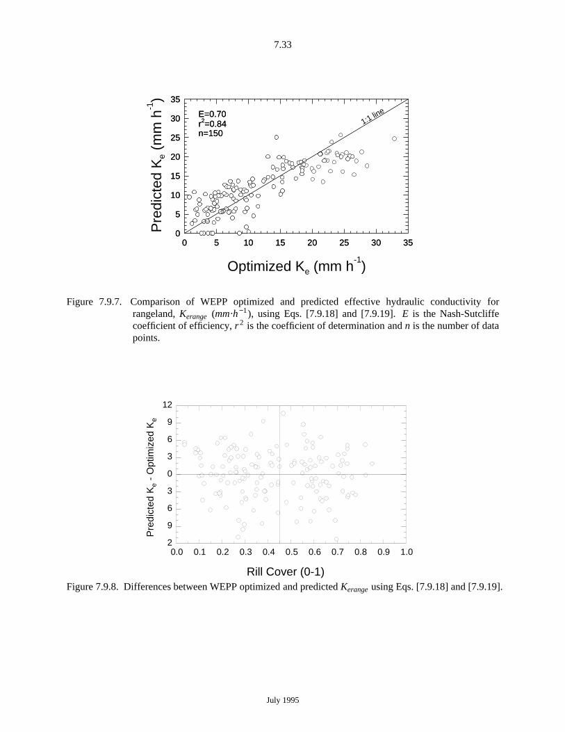
7.33

Pre

dict

ed K

e(m

m h

-1)

0 5 10 15 20 25 30 350

5

10

15

20

25

30

35

E=0.70r2=0.84n=150

0 5 10 15 20 25 30 350

5

10

15

20

25

30

35

E=0.70r2=0.84n=150

Optimized Ke (mm h-1)

1:1 line

Figure 7.9.7. Comparison of WEPP optimized and predicted effective hydraulic conductivity forrangeland, Kerange (mm.h −1), using Eqs. [7.9.18] and [7.9.19]. E is the Nash-Sutcliffecoefficient of efficiency, r 2 is the coefficient of determination and n is the number of datapoints.

0.0 0.1 0.2 0.3 0.4 0.5 0.6 0.7 0.8 0.9 1.02

9

6

3

0

3

6

9

12

Pre

dict

ed K

e-

Opt

imiz

ed K

e

Rill Cover (0-1)Figure 7.9.8. Differences between WEPP optimized and predicted Kerange using Eqs. [7.9.18] and [7.9.19].

July 1995

7.34

0 5 10 15 20 25 300

5

10

15

20

25

30

E=0.34r2=0.63n=150

Observed Runoff (mm)

Pre

dict

ed R

unof

f (m

m)

1:1 line

Figure 7.9.9. Comparison of WEPP predicted runoff using Kerange values estimated using Eqs. [7.9.18]and [7.9.19] and observed runoff. The data set of observed runoff is from the same plotsthat Eqs. [7.9.18] and [7.9.19] were developed. E is the Nash-Sutcliffe coefficient ofefficiency, r 2 is the coefficient of determination and n is the number of data points.

Observed Peak Runoff (mm h

-1-1

-1-1)0 10 20 30 40 50 60

0

10

20

30

40

50

60

70E=0.26r2=0.52n=126

Pre

dict

ed P

eak

Run

off (

mm

h

)

1:1 line

Figure 7.9.10. Comparison of WEPP predicted peak runoff using Kerange values estimated using Eqs.[7.9.18] and [7.9.19] and observed runoff. The data set of observed peak runoff is fromthe same plots that Eqs. [7.9.18] and [7.9.19] were developed. E is the Nash-Sutcliffecoefficient of efficiency, r 2 is the coefficient of determination and n is the number of datapoints. The number of data points shown is 126 because 24 plots had zero predictedrunoff.

July 1995

7.35

7.9.7 Freeze and Thaw Adjustments to Conductivity Values

The WEPP winter component (Chapter 3) computes frost and thaw development in the soil. Whenthe soil is totally or partially frozen, an adjustment is made within the model to the hydraulic conductivityvalues used in the infiltration and percolation calculations.

The hydraulic conductivity adjustment for frozen soil (FSa) is predicted from (Lee, 1983):

FSa = 3.75 e−0.26Fθ [7.9.20]

F θ is predicted from:

F θ =θfc

θfhhh100 [7.9.21]

where θf is the volumetric soil water content at freezing (m3.m−3) and θfc is the volumetric soil watercontent at field capacity. If F θ is greater than or equal to 100, FSa is set equal to 0.1.

For the frozen soil layer, conductivity will be calculated using the equation

Kfrozen = Kunfrozen(FSa) [7.9.22]

where Kfrozen represents the hydraulic conductivity that will be used for the frozen soil layer (mm.h −1),and Kunfrozen is the hydraulic conductivity of the soil in an unfrozen condition (mm.h −1). If part of a soillayer is frozen, a weighted average (by frozen/unfrozen thickness) of the frozen and unfrozenconductivities is used for the infiltration and/or percolation computations.

7.10 Interrill Erodibility Parameters

7.10.1 Cropland Baseline Interrill Erodibility

The WEPP model is very sensitive to the input values for the soil erodibility parameters. The usermust input a value for the baseline interrill erodibility (Kib), which represents the erodibility of a freshly-tilled soil. If the user enters a value of 0.0 for Kib in the soil input file, the baseline interrill erodibility fora cropland simulation will be set to 5,300,000 kg .s .m−4.

A series of field experiments was conducted in 1987 and 1988 to develop estimation equations forerodibility parameters (Elliot et al., 1989). For cropland surface soils containing 30% or more sand, theequation for baseline interrill erodibility is:

Kib = 2728000 + 19210000 vfs [7.10.1]

where vfs is the fraction of very fine sand in the surface soil. If very fine sand content is greater than 0.40,use a maximum value of 0.40 in the equation.

For soils containing less than 30% sand, the equation is

Kib = 6054000 − 5513000 clay [7.10.2]

where clay is the fraction of clay in the surface soil. If clay content is less than 0.10, use 0.10 in theequation. Be sure to check the most recent version of the WEPP user summary document for any changesor updates to these equations. Table 7.10.1 provides suggested limits for Kib values.

July 1995

7.36

Table 7.10.1. Suggested limits for baseline values for Ki, Kr, and τc for cropland.iiiiiiiiiiiiiiiiiiiiiiiiiiiiiiiiiiiiiiiiii

Kib Krb τcb(kg .s .m−4) (s .m−1) (Pa)iiiiiiiiiiiiiiiiiiiiiiiiiiiiiiiiiiiiiiiiii

Minimum Value 500000 .002 0.3Maximum Value 12000000 .050 7.0iiiiiiiiiiiiiiiiiiiiiiiiiiiiiiiiiiiiiiiiii

7.10.2 Cropland Interrill Erodibility Adjustments

The baseline interrill erodibility on croplands is multiplied by an assortment of adjustment factorsto account for various effects, including canopy cover, ground cover, roots, and sealing and crusting. Thefinal adjusted interrill erodibility which is used on a day during a WEPP simulation is:

Kiadj = Kib (CKican) (CKigc) (CKidr) (CKilr) (CKisc) (CKisl) (CKift)[7.10.3]

where Kiadj is the adjusted interrill erodibility. The individual adjustment factors are described below.

7.10.2.1 Canopy Effects

The canopy adjustment factor, CKican , for Kib is predicted from

CKican = 1 − 2.941h

cancovhhhhhhh IL1 − e−0.34h M

O[7.10.4]

where h is the canopy height in meters.

7.10.2.2 Ground Cover

The ground cover adjustment factor (CKigc) for Ki is predicted from

CKigc = e−2.5 inrcov [7.10.5]

where inrcov is the interrill cover (0-1).

7.10.2.3 Roots

Effects of dead and live root biomass within the 0- to 0.15-m soil zone on interrill erodibility of acropland soil are predicted separately. The effect of dead roots on interrill erodibility is predicted:

CKidr = e−0.56 dr [7.10.6]

where CKidr is the interrill erodibility adjustment for dead roots and dr is dead root mass (kg .m−2) withinthe 0- to 0.15-m soil zone.

The effect of live roots on interrill erodibility is predicted from:

CKilr = e−0.56 lr [7.10.7]

where CKilr is the interrill erodibility adjustment for live roots and lr is live root biomass (kg .m−2) withinthe 0- to 0.15-m soil zone.

There is no adjustment to account for the effect of buried residues on interrill erodibility.

July 1995

7.37

7.10.2.4 Sealing and Crusting

The effect of sealing and crusting on interrill erodibility is predicted from:

CKisc =Kib

Kiconshhhhhh +IJL1 −

Kib

KiconshhhhhhMJOe−ρc daydis [7.10.8]

where CKisc is the adjustment factor, Kib is the baseline interrill erodibility, daydis is the cumulativenumber of days since total soil disturbance, and Kicons is the consolidated interrill erodibility and iscalculated as:

Kicons = 103 (3042 − 3166 sand − 8816 orgmat − 2477 θcf)[7.10.9]

7.10.2.5 Interrill Slope Adjustment

The interrill slope adjustment factor (CKisl) is calculated as:

CKisl = 1.05 − 0.85 e 4 sinΩ [7.10.10]

where Ω is the interrill slope angle. If the interrill slope angle is less than the average OFE slope, theaverage OFE slope is used in place of Ω in Eq. [7.10.10].

7.10.2.6 Freeze and Thaw

Soil that has undergone one or more freeze-thaw cycles is normally in a more erodible conditionafter thawing, at least until the soil dries. Adjustments to baseline interrill erodibility, rill erodibility, andcritical shear stress are made from the time a frozen soil thaws until it dries to less than 1/3 bar watercontent. The adjustment equation is initially a function of the number of freeze-thaw cycles, until amaximum of 10 cycles have occurred during the current winter period.

CKift = acyc e−ln

IJL(acyc)

33

ΨsurfhhhhhMJO

[7.10.11]

where CKift is the interrill adjustment factor due to freeze-thaw, Ψsurf is the soil matric potential in thesurface soil layer (KPa), and acyc is the freeze-thaw cycle factor. acyc is computed using:

acyc = 1 + 0.0586 (cycles) − 0.0027 (cycles)2 [7.10.12]

where cycles is the number of freeze-thaw cycles in the current winter period. When cycles exceed 10,acyc is set to a constant 1.31.

7.10.3 Rangeland Baseline Interrill Erodibility

Data collected from a study of 18 rangeland sites (Simanton et al., 1987) in 1987 and 1988 wereanalyzed to develop a relationship between interrill erodibility and soil physical and chemical properties.

The baseline Ki is predicted from:

Ki = 1000 [ 1810 − 1910 sand − 6327 orgmat − 846 θfc ] [7.10.13]

where Ki is the baseline interrill erodibility parameter for a rangeland soil (kg .s .m−4), sand is the fractionof sand (0 to 1), orgmat is the fraction of organic matter (0 to 1), and θfc is the volumetric water contentof the soil at 0.033 MPa (m3.m−3). If the predicted Ki is < 10,000 kg .s .m−4, then Ki is set equal to10,000. If Ki is > 2,000,000 kg .s .m−4, then Ki is set equal to 2,000,000.

July 1995

7.38

Table 7.10.2 gives the optimized erodibility values from the WEPP rangeland field studies. Table7.10.3 gives the ranges of the variables used in developing Eq. [7.10.13]. It is recommended that Eq.[7.10.13] not be used with input data outside these ranges. Figure 7.10.1 compares the measured andpredicted values of Ki . Table 7.10.4 lists the recommended upper and lower limits for rangeland Ki .

Table 7.10.2. Location and soil series description of mean site optimized interrill erodibility, Ki(kg .s .m−4), rill erodibility, Kr (s .m−1), and critical shear stress, τc (Pa) from USDArangeland rainfall simulation experiments.

iiiiiiiiiiiiiiiiiiiiiiiiiiiiiiiiiiiiiiiiiiiiiiiiiiiiiiiiiiiiiiiiiiiiiiiiiiiiiiiiiiiiiiiiiiiiiiiiiOptimized Optimized Optimized

Location1 Soil family Soil series Surface texture Ki* Kr* τciiiiiiiiiiiiiiiiiiiiiiiiiiiiiiiiiiiiiiiiiiiiiiiiiiiiiiiiiiiiiiiiiiiiiiiiiiiiiiiiiiiiiiiiiiiiiiiii3) Tombstone, AZ Ustochreptic calciorthid Stronghold Sandy loam 285 5.3 0.5024) Tombstone, AZ Ustollic haplargid Forest Sandy clay loam 263 3.5 1.3065) Susanville, CA Typic argixeroll Jauriga Sandy loam 270 1.2 0.313

10) Meeker, CO Typic camborthid Degater Silty clay 1195 16.2 4.36014) Sidney, MT Typic argiboroll Vida Loam 315 3.2 0.02517) Cuba, NM Ustollic camborthid Querencia Sandy loam 445 1.7 0.57618) Los Alamos, NM Aridic haplustalf Hackroy Sandy loam 485 2.1 0.52821) Chickasha, OK Udic argiustoll Grant Loam3 357 1.5 1.16022) Chickasha, OK Udic argiustoll Grant Sandy loam 422 1.1 0.71223) Freedom, OK Typic ustochrept Woodward Loam 972 1.0 0.05024) Woodward, OK Typic ustochrept Quinlan Loam 469 8.3 1.88025) Cottonwood, SD Typic torrert Pierre Clay 1030 2.0 0.42626) Cottonwood, SD Typic torrert Pierre Clay 947 1.5 3.27035) Mercury, NV NA4 NA Sandy loam 223 4.6 0.13636) Mercury, NV Thermic nadurargid NA Gravelly sandy loam 186 3.3 0.28837) Ft. Supply, OK Thermic haplustalf Pratt Sand 20 30.2 5.71038) Freedom, OK Thermic ustochrept Woodward Loam 903 0.9 0.00139)Los Banos, CA Thermic haploxeroll Apollo Loam 238 0.4 0.031iiiiiiiiiiiiiiiiiiiiiiiiiiiiiiiiiiiiiiiiiiiiiiiiiiiiiiiiiiiiiiiiiiiiiiiiiiiiiiiiiiiiiiiiiiiiiiiii

* Ki times 1,000 equals measured Ki . Kr divided by 10,000 equals measured Kr .

1 Locations numbers in this table are consistant with location references in rangeland plant growth and effective hydraulicconductivity (Kerange) tables and therefore are not numbered sequentially in this table. Locations 35 through 39 were used todevelop soil erodibility coefficients for the WEPP model but were not used to develop Kerange .

2 Farm land abandoned during the 1930’s that had returned to rangeland. The majority of the ‘A’ horizon had been previouslyeroded.

3 NA indicates data not available.

Table 7.10.3. Ranges of the variables used to develop Eq. [7.10.13].iiiiiiiiiiiiiiiiiiiiiiiiiiiiiiiii

Variable Range Unitsiiiiiiiiiiiiiiiiiiiiiiiiiiiiiiiii

sand 0.08 to 0.88 (Fraction)orgmat 0.005 to 0.112 (Fraction)θfc 0.04 to 0.40 (m3.m−3)iiiiiiiiiiiiiiiiiiiiiiiiiiiiiiiii

July 1995

7.39

1,400,000

1,200,000

1,000,000

800,000

600,000

400,000

200,000

00 200,000 400,000 600,000 800,000 1,000,000 1,200,000 1,400,000

r = 0.762

n = 181:1

MEASURED Ki (kg s m ) -4

PR

ED

ICT

ED

Ki (

kg s

m

)

-4

Figure 7.10.1. Rangeland measured vs. predicted Ki for eighteen WEPP field study sites.

Table 7.10.4. Suggested limits for predicted values for Ki , Kr , and τc for rangeland.iiiiiiiiiiiiiiiiiiiiiiiiiiiiiiiiiiiiiiiiiiiiiii

Ki Kr τc(kg .s .m−4) (s .m−1) (pascals)iiiiiiiiiiiiiiiiiiiiiiiiiiiiiiiiiiiiiiiiiiiiiii

Minimum Value 10000 0.00001 0.3Maximum Value 2000000 0.004 7iiiiiiiiiiiiiiiiiiiiiiiiiiiiiiiiiiiiiiiiiiiiiii

7.10.4 Rangeland Interrill Erodibility Adjustments

Baseline interrill soil erodibility for rangelands is adjusted in a similar way to croplands, only thereare currently less adjustment factors:

Kiadj = Kib (RKicov) (RKift)[7.10.14]

where Kiadj is the adjusted interrill erodibility, Kib is the baseline interrill erodibility for the rangelandsoil, RKicov is the adjustment factor for rangeland cover, and RKift is the adjustment for freezing andthawing.

7.10.4.1 Ground Cover Adjustment

The rangeland cover adjustment factor (RKicov) for Kib is predicted from:

RKicov = e−7.0(inrcov + cancov) [7.10.15]

where inrcov is the interrill cover (0-1) and cancov is the canopy cover (0-1).

7.10.4.2 Freeze and Thaw

Freeze and thaw adjustment relationships for cropland interrill erodibility, that are given in Eq.[7.10.11] are also applied to rangeland soils within a WEPP model simulation. Thus, RKift = CKift in theWEPP model.

July 1995

7.40

7.11 Rill Erodibility Parameters

7.11.1 Baseline Rill Erodibility and Critical Shear for Cropland Soils

The WEPP model is very sensitive to the input values for baseline rill erodibility and critical shearstress. Baseline erodibility parameters in cropland simulations are meant to represent the erodibilitycharacteristics of a freshly-tilled soil. A baseline rill erodibility (Krb) and a baseline critical hydraulicshear stress (τcb) must be supplied to the model in the soil input file by the user. If the user enters 0.0, theWEPP model sets the value of Krb and τcb to 0.0115 s .m−1 and 3.1 pascals, respectively.

A set of field experiments conducted in 1987 and 1988 (Elliot et al., 1989). was used to derive thefollowing equations, which can be used to estimate Krb and τcb. For cropland surface soils containing30% or more sand, the equations are:

Krb = 0.00197 + 0.030 vfs + 0.03863 e−184 orgmat [7.11.1]

τcb = 2.67 + 6.5 clay − 5.8 vfs [7.11.2]

where vfs is the fraction of very fine sand in the surface soil, clay is the fraction of clay in the surface soil,and orgmat is the fraction of organic matter in the surface soil. In the development of these equations,organic matter (orgmat) was assumed to be equal to 1.724 times the organic carbon content (orgc). Ifvery fine sand content is less than 0.40, use 0.40 in the equations. If clay content is more than 0.40, use0.40 in the equation. If organic matter content is less than 0.0035, use 0.0035 in the equation.

For cropland soils containing less than 30% sand,

Krb = 0.0069 + 0.134 e−20 clay [7.11.3]

τcb = 3.5 [7.11.4]

If clay content is less than 0.10, use 0.10 in the equation.

Be sure to check the most recent WEPP user summary documentation for any changes or updates tothese equations.

7.11.2 Cropland Rill Erodibility Adjustments

The baseline rill erodibility in the WEPP model is multiplied by a set of adjustment factors toaccount for various temporally-changing factors, including incorporated residue, roots, sealing andcrusting, and freezing and thawing. The final adjusted rill erodibility for croplands which is used on asimulation day to predict rill detachment is:

Kradj = Krb (CKrbr) (CKrdr) (CKrlr) (CKrsc) (CKrft)[7.11.5]

where Kradj is the adjusted rill erodibility, Krb is the baseline rill erodibility, and the other terms are themultiplicative adjustment factors described below.

7.11.2.1 Incorporated Residue

The following relationship is used to predict the effect of incorporated residue on Kr for acropland soil

July 1995

7.41

CKrbr = e−0.4br [7.11.6]

where CKrbr is the rill erodibility adjustment for buried residue and br is the mass of buried residue(kg .m−2) within the 0- to 0.15-m soil zone. This adjustment factor is based on the work of Alberts andGantzer (1988) and Brown and Foster (1987).

7.11.2.2 Roots

The adjustments to Kr for dead roots (CKrdr) and live roots (CKrlr) are given as:

CKrdr = e−2.2dr [7.11.7]

where dr is the mass of dead roots (kg .m−2)

CKrlr = e−3.5lr [7.11.8]

where lr is mass of living roots (kg .m−2) within the 0- to 0.15-m soil zone.

7.11.2.3 Sealing and Crusting

The adjustment to Kr due to sealing and crusting (CKrsc) is estimated by:

CKrsc =Kr

Krconshhhhhh +IJL1 −

Kr

KrconshhhhhhMJOe−ρc daydis [7.11.9]

where Krcons is the consolidated rill erodibility and is predicted from:

Krcons = 0.00035 − 0.0014 θcf + 0.00068 silt + 0.0049 Mcf[7.11.10]

7.11.2.4 Freeze and Thaw

The adjustment for rill erodibility as the soil dries from saturation to field capacity is:

CKrft = 2.0 (0.933)Ψsurf [7.11.11]

where Ψsurf is the matric potential of the surface soil in KPa. Once the soil dries to field capacity, nofurther adjustment is made unless the soil surface becomes frozen then thaws once more.

7.11.3 Cropland Critical Hydraulic Shear Adjustments

As with the interrill and rill erodibilities, the baseline critical shear stress is multiplied by a set ofadjustment factors to account for temporal variations in τc. The final adjusted τc value used on a day ofsimulation in the WEPP model is:

τcadj = τcb (Cτrr) (Cτsc) (Cτcons) (Cτ ft)[7.11.12]

where τcadj is the adjusted critical shear stress value, τcb is the baseline critical shear stress value, and themultiplicative factors are as described below.

July 1995

7.42

7.11.3.1 Random Roughness

The effect of random roughness on critical shear is calculated as:

Cτrr = 1.0 + 8.0 (RRt − 0.006) [7.11.13]

where RRt is the random roughness of the surface soil (mm).

7.11.3.2 Sealing and Crusting

The adjustment to τc due to sealing and crusting (Cτsc) is predicted from:

Cτsc =τc

τconshhhhh +IJL1 −

τc

τconshhhhhMJOe−ρc daydis [7.11.14]

where τcons is the consolidated critical shear and is calculated as:

τcons = 8.37 − 11.8 θfc − 4.9 sand [7.11.15]

7.11.3.3 Freeze and Thaw

The adjustment to critical hydraulic shear stress for freezing and thawing effects is given by:

Cτ ft = 0.875 + 0.0543 ln(Ψsurf)[7.11.16]

where Cτ ft is the adjustment factor for critical shear stress and Ψsurf is the matric potential of the surfacesoil (KPa). The adjustment becomes inactive once the soil becomes drier than field capacity (1/3 barwater content), and does not become active again until the soil has frozen and is thawing again.

7.11.4 Baseline Rill Erodibility and Critical Shear for Rangeland Soil

Data collected from a study of 18 rangeland soils (Simanton et al., 1987) conducted in 1987 and1988 were analyzed to develop relationships between rill erodibility and critical shear stress and soilphysical and chemical properties.

Baseline Kr for rangelands is predicted from:

Kr = 0.0017 + 0.0024 clay − 0.0088 orgmat −1000

0.00088 ρdhhhhhhhhhh − 0.00048 ROOT 10[7.11.17]

where Kr is the baseline rill erodibility for rangeland (s .m−1), clay is soil clay content (0-1), orgmat isorganic matter content of the surface soil (0-1), ρd is dry soil bulk density (kg .m−3), and ROOT 10 is totalroot mass in the top 10 cm of the soil surface (kg .m−2).

Table 7.11.1 gives the ranges of the variables used in developing Eq. [7.11.17]. It is recommendedthat Eq. [7.11.17] not be used with input data outside these ranges. The recommended lower and upperlimits for rangeland Kr are given in Table 7.10.4.

July 1995

7.43

Table 7.11.1. Ranges of the variables used to develop Eq. [7.11.17].iiiiiiiiiiiiiiiiiiiiiiiiiiiiiiiiiiiiiiiiiiiiiii

Variable Range Unitsiiiiiiiiiiiiiiiiiiiiiiiiiiiiiiiiiiiiiiiiiiiiiii

clay 0.033 to 0.422 Fractionorgmat 0.005 to 0.112 FractionROOT 10 0.02 to 4.10 kg .m−2

ρd 1200 to 1800 kg .m−3iiiiiiiiiiiiiiiiiiiiiiiiiiiiiiiiiiiiiiiiiiiiiii

Critical shear stress can be predicted using:

τc = 3.23 − 5.6 sand − 24.4 orgmat +1000

0.9ρdhhhhhh [7.11.18]

where τc is the critical shear stress of the flow necessary to detach soil (Pa) and sand is the fraction ofsand in the surface soil (0 to 1).

Table 7.11.2 gives the ranges of the variables used in developing Eq. [7.11.12]. It is recommendedthat Eq. [7.11.12] not be used with input data outside these ranges. The recommended lower and upperlimits for rangeland τc are given in Table 7.10.3.

Table 7.11.2. Ranges of the variables used to develop Eq. [7.11.18].iiiiiiiiiiiiiiiiiiiiiiiiiiiiiiiiiiiiiiiiiiiiiiVariable Range Unitsiiiiiiiiiiiiiiiiiiiiiiiiiiiiiiiiiiiiiiiiiiiiiisand 0.08 to 0.88 Fractionorgmat 0.005 to 0.112 Fractionρd 1200 to 1800 kg .m−3iiiiiiiiiiiiiiiiiiiiiiiiiiiiiiiiiiiiiiiiiiiiii

7.11.5 Rangeland Kr and τc Adjustments

Currently the only adjustment made to the baseline rangeland rill erodibility and critical shearstress parameters are due to soil freezing and thawing effects. The freeze and thaw adjustmentrelationships for cropland rill erodibility and critical shear given in Eqs. [7.11.11] and [7.11.16],respectively, are also applied in rangeland simulations in the WEPP model.

7.12 References

Alberts, E.E. and C.J. Gantzer. 1988. Influence of incorporated residue and soil consolidation on rill soilerodibility. Agronomy Abstracts. p. 270.

Bosch, D.D. and C.A. Onstad. 1988. Surface seal hydraulic conductivity as affected by rainfall. Trans.ASAE 31(4):1120-1127.

Brakensiek, D.L. and W.J. Rawls. 1983. Agricultural management effects on soil water processes PartII: Green and Ampt parameters for crusting soils. Trans. ASAE 26(6):1753-1759.

Brakensiek, D.L., W.J. Rawls and G.R. Stephenson. 1986. Determining the saturated hydraulicconductivity of soil containing rock fragments. Soil Sci. Soc. Am. J. 50(3):834-835.

Brown, L.C. and G.R. Foster. 1987. Rill erosion as affected by incorporated crop residue. ASAE PaperNo. 87-2069, American Society of Agricultural Engineers, St. Joseph, MI.

July 1995

7.44

Eigel, J.D. and I.D. Moore. 1983. Effect of rainfall energy on infiltration into a bare soil. In: Proc. ofASAE conference on Advances in Infiltration, Chicago, IL. pp.188-199.

Elliot, W.J., K.D. Kohl and J.M. Laflen. 1988. Methods of collecting WEPP soil erodibility data. ASAEPaper No. MCR 88-138, American Society of Agricultural Engineers, St. Joseph, MI.

Elliott, W.J., A.M. Liebenow, J.M. Laflen and K.D. Kohl. 1989. A Compendium of Soil ErodibilityData From WEPP Cropland Soil Field Erodibility Experiments 1987 & 1988. NSERL Report No.3, USDA-ARS National Soil Erosion Research Lab., West Lafayette, IN.

Khan, M.J., E.J. Monke and G.R. Foster. 1988. Mulch cover and canopy effects on soil loss. Trans.ASAE 31(3):706-711.

Laflen, J.M., A.W. Thomas and R.W. Welch. 1987. Cropland Experiments for the WEPP project.ASAE Paper No. 87-2544, American Society of Agricultural Engineers, St. Joseph, MI.

Laws, J.O. 1941. Measurements of the fall-velocity of water-drop and raindrops. Trans. Am.Geophysical Union 22:706-721.

Lee, H.W. 1983. Determination of infiltration characteristics of a frozen Palouse silt loam soil undersimulated rainfall. Ph.D. Dissertation, University of Idaho, Moscow, Idaho.

Onstad, C.A., M.L. Wolf, C.L. Larson and D.C. Slack. 1984. Tilled soil subsidence during repeatedwetting. Trans. ASAE 27(3):733-736.

Potter, K.N. 1990. Soil properties effect on random roughness decay by rainfall. Trans. ASAE33(6):1889-1892.

Rawls, W.J. and D.L. Brakensiek. 1983. A procedure to predict Green and Ampt infiltration parameters.Proc. of ASAE conference on Advances in Infiltration, Chicago, IL. pp.102-112.

Rawls, W.J., D.L. Brakensiek, J.R. Simanton and K.D. Kohl. 1990. Development of a Crust Factor forthe Green Ampt Model. Trans. ASAE 33(4):1224-1228.

Risse, L.M. 1994. Validation of WEPP using Natural Runoff Plot Data. Unpubl. Ph.D. dissertation.National Soil Erosion Research Laboratory, Purdue University, West Lafayette IN. 230 pp.

Simanton, J.R., L.T. West, M.A. Weltz and G.D. Wingate. 1987. Rangeland experiment for the WEPPproject. ASAE Paper No. 87-2545. American Society of Agricultural Engineers, St. Joseph, MI.

Van Doren, D.M. and R.R. Allmaras. 1978. Effect of Residue Management Practices on the soilphysical environment, micro climate, and plant growth. Am. Soc. Agron. Spec. Publ. #31. CropResidue Systems. ASA, CSSA, SSSA, Madison, WI. pp. 49-83.

Williams, J.R., C.A. Jones and P.T. Dyke. 1984. A modeling approach to determining the relationshipbetween erosion and soil productivity. Trans. ASAE 27(1):129-142.

Wischmeier, W.H. 1966. Surface runoff in relation to physical and management factors. Proc. First PanAmerican Soil Conservation Congress. San Paulo, Brazil. p. 237-244.

July 1995

7.45

7.13 List of Symbols

Symbol Definition Units Variable

acyc Freeze-thaw cycle factor - acycb Adjustment coefficient for random roughness - crrBASCOV Total basal surface cover fraction (0-1) Fraction bascovBASI Fraction of basal surface cover in interrill areas Fraction basiBASR Fraction of basal surface cover in rill areas Fraction basrbr Mass of buried residue within the 0- to 0.15 m soil zone kg .m −2 smrmc Coefficient relating amount of kinetic energy since last tillage m 2.J −1 cke

to the speed of crust formationcancov canopy cover Fraction cancovCbr Random roughness and ridge height adjustment factor for buried residue Fraction cbrccovef Effective canopy cover Fraction ccovefCEC Cation exchange capacity meq /100g cecCECc Cation exchange capacity of clay meq /100g ceccCECr CECc/clay meq /100g solconCF Crust factor Fraction crustCh Hydraulic conductivity adjustment factor for canopy height Fraction -CKican Cropland interrill erodibility adjustment factor for canopy cover Fraction ckiaccCKidr Cropland interrill erodibility adjustment factor for dead root Fraction ckiadrCKift Cropland interrill erodibility adjustment factor for freeze and thaw Fraction ckiaftCKigc Cropland interrill erodibility adjustment factor for ground cover Fraction ckiagcCKilr Cropland interrill erodibility adjustment factor for live roots Fraction ckialrCKisc Cropland interrill erodibility adjustment factor for sealing and crusting Fraction ckiascCKisl Cropland interrill erodibility adjustment factor for slope Fraction ckiaslCKrbr Cropland interrill erodibility adjustment factor for residue Fraction ckiabrCKrdr Cropland interrill erodibility adjustment factor for dead roots Fraction ckiadrCKrft Cropland rill erodibility adjustment factor for freeze and thaw Fraction ckraftCKrlr Cropland rill erodibility adjustment factor for live roots Fraction ckalrCKrsc Cropland interrill erodibility adjustment factor for sealing and crusting Fraction ckrascclay Clay content of the soil Fraction clayCN Curve number - -Cτ ft Critical shear adjustment factor for freeze and thaw Fraction tcaftCτrr Critical shear adjustment factor for random roughness Fraction tcarrCτsc Critical shear adjustment factor for sealing and crusting Fraction tcasccycles Number of freeze-thaw cycles in current winter period - cycledaycnt Counter to track the number of days since the last tillage operation d daycntdaydis The number of days since disturbance d daydisDg Depth of the soil horizon of interest m dgdr Amount of dead root mass kg .m −2 rtmEa Cumulative kinetic energy of the rainfall since the last tillage operation J .m −2 rkecumFa Volume of entrapped air in the soil Fraction cocaFcf Correction for the volume of coarse fragment in the soil Fraction cpmFdc Daily soil bulk density consolidation factor Fraction dayconF θ Ratio of soil water content at freezing to % -

to the soil water content at field capacityFSa Hydraulic conductivity adjustment for frozen soil Fraction frofFBASI Basal surface cover area fraction on the interrill areas Fraction fbasiFBASR Basal surface cover area fraction in the rill channels Fraction fbasr

July 1995

7.46

FRESI Residue cover area fraction on interrill areas Fraction fresiFRESR Residue cover area fraction in the rill channels Fraction fresrh Canopy height m canhgtinrcov Interrill cover Fraction inrcovKappr Approximation of hydraulic conductivity for each event under mm .h −1 -

meadow conditionKb Baseline effective hydraulic conductivity mm .h −1 avksKbare Effective Kb after adjustment for crusting and tillage mm .h −1 kbareKe Effective hydraulic conductivity in fill layer mm .h −1 ekeKec Time-invariant effective hydraulic condutivity mm .h −1 -Kef Effective hydraulic conductivity for fallow soil conditions mm .h −1 -Kerange Effective hydraulic conductivity for rangeland soils mm .h −1 -Ki Interrill soil erodibility kg .s.m −4 -Kiadj Adjusted interrill soil erodibility kg .s.m −4 kiadjf*kiKib Baseline interrill soil erodibility kg .s.m −4 kiKicons Consolidated interrill soil erodibility kg .s.m −4 kconsdKr Rill soil erodibility s.m −1 -Kradj Adjusted rill soil erodibility s.m −1 kradjf*krKrb Baseline rill soil erodibility s.m −1 krKrcons Consolidated rill soil erodibility s.m −1 kconsdKunfrozen Hydraulic conductivity of soil in unfrozen condition mm .h −1 sscunfKfrozen Hydraulic conductivity of soil in frozen condition mm .h −1 -L Depth of wetting front m wetfrtlr Amount of live root mass kg .m −2 rtm15Mcf Coarse fragment content by weight Fraction rfgME Nash-Sutcliffe model efficiency - -Ω Interrill slope angle rad -orgc Organic carbon content Fraction orgcorgmat Organic matter content Fraction orgmatφe Effective porosity Fraction eporφt Total porosity Fraction porρc Consolidated soil bulk density at 0.033 MPa kg .m −3 bdcons∆ρc Difference in bulk density between a soil that is naturally kg .m −3 bddiff

consolidated and one that has received 0.1 m of rainfallρd Soil bulk density at the wilting point kg .m −3 bddry∆ρmx Maximum increase in soil bulk density with rainfall kg .m −3 Ao

∆ρrf Adjustment for increasing bulk density due to consolidation by rainfall kg .m −3 bdrifρt Soil bulk density after tillage kg .m −3 bdtill∆ρwt Daily increase in soil bulk density after 0.1 m of rainfall kg .m −3 bdiwtρb Bulk density kg .m −3 bdrain Storm rainfall amount mm rainRESI Fraction of litter surface cover on interrill areas Fraction resiRKicov Interrill erodibility adjustment factor for rangeland cover Fraction rkiagcRKift Interrill erodibility adjustment for freezing and thawing Fraction rkiaftRc Cumulative rainfall since tillage m rfcumrescov Residue cover Fraction rescovRHo Ridge height immediately after tillage m rhoRHt Ridge height at time t m rhROOT 10 Total live and dead root mass in the top 0.1 m of soil kg .m −2 rootyRR Random roughness of the soil m -RRt Random roughness at time t m rrc

July 1995

7.47

RRi Random roughness immediately after tillage m rrinitRRo Random roughness of a tillage implement m rrosand sand content Fraction sandSC Correction factor for partial saturation of the subcrust soils Fraction scscovef Total effective surface cover Fraction scovefsilt Silt content Fraction siltTds Fraction of the soil surface disturbed by a tillage implement Fraction surdisτ Shear stress of the flow Pa tauτc Critical shear stress of the flow necessary to initiate detachment Pa -τcadj Adjusted critical shear stress Pa tcadjf*shcritτcb Baseline critical shear stress Pa shcritτcons Consolidated critical shear stress Pa kconsdθ Soil water content by volume Fraction thetθd Soil water content at 1.5 MPa by volume Fraction thetdrθf Soil water content at freezing by volume Fraction smfθfc Soil water content at 0.033 MPa by volume Fraction thetfcθr Residual water content by volume Fraction wrdVcf Coarse fragment content by volume Fraction vcfvfs Fracton of very fine sand in surface soil Fraction -Ψ Steady state capillary potential at the crust/subcrust interface - ffiΨsurf Soil matric potential in the surface soil layer KPa tenkpa

July 1995