Plumbing

103

Chapter 7 Plumbing

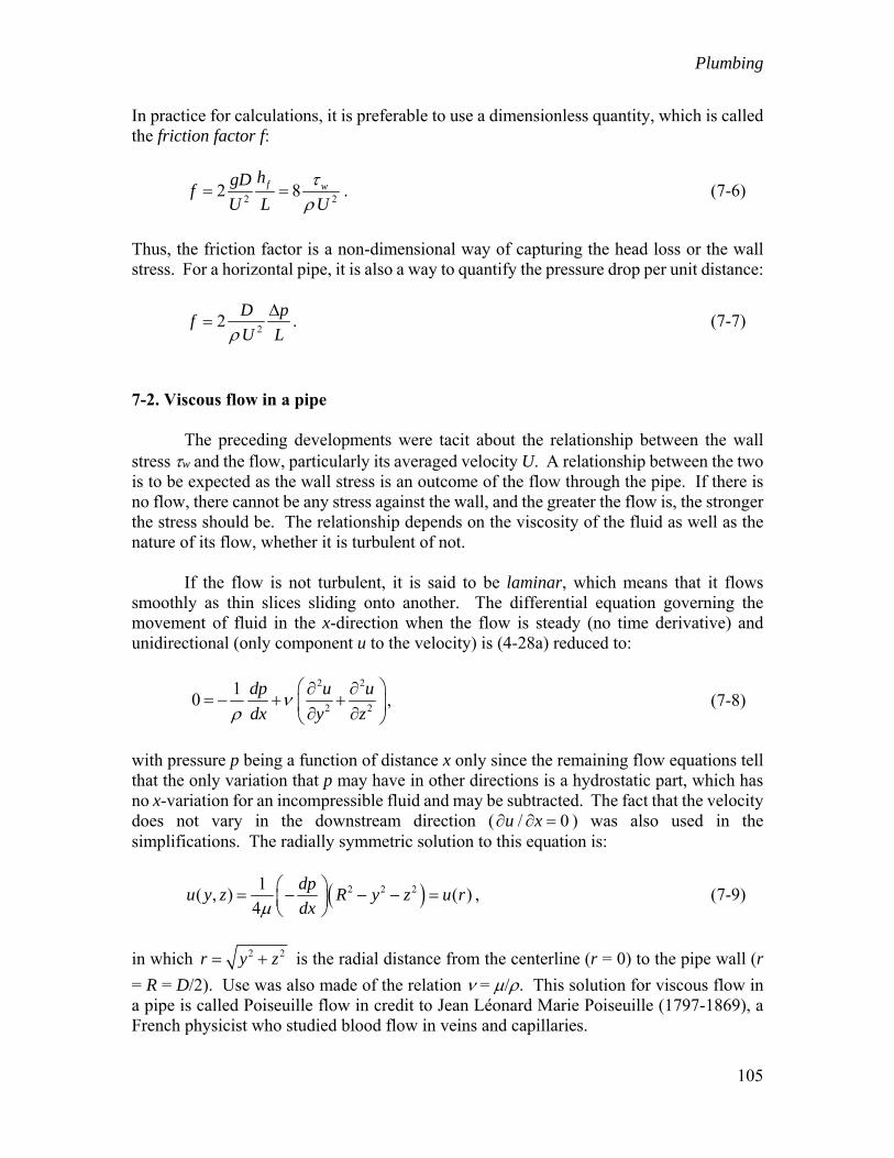
7-1. Flow down a pipe Throughout this chapter, we will assume that the fluid is incompressible. This is easy to justify when the fluid is water (which is the most common situation) or another liquid, but it turns out also to be a good approximation when the fluid is a gas as long as its speed is much less than the sound speed. Compressible gas flow is considered in Chapter 17 Rocket Science because it occurs in rocket engines. Incompressibility reduces mass conservation to volume conservation: The volumetric flow rate Q along a single pipe is conserved. As an initial step, we further limit ourselves to circular pipes with uniform inner diameter D. Conservation of volumetric flow rate in a pipe of unchanging cross-section implies conservation of velocity: The velocity distribution u(r) as a function of radial distance r from center across the pipe’s section, and thus also the averaged velocity U, remains unchanged with distance along the pipe. It follows that there is no acceleration or deceleration in such a pipe flow and that the several existing forces must balance one another. There are three forces acting on pipe flow: the pressure that “pushes” the flow through the pipe, wall friction that acts against the flow, and gravity if the pipe is inclined. The situation is depicted in Figure 7-1.

Figure 7-1. Force balance over a section of a circular pipe.

The pressure force is the pressure times the cross-sectional area D2/4, and the difference between the forward pressure p on the upstream side and the backward pressure p – p on the downstream side is +p. Thus, the net pressure force is 2( / 4)D p . The frictional

Plumbing

104

force is the wall stress w times the peripheral area DL, while the gravitational force is the weight mg = (D2L/4)g times the sinus of the inclination angle . The overall force balance is:

2 2

sin4 4w

D D Lp DL g

,

which can be reduced to:

4

sinw

pg

L D

. (7-1)

The ratio p/L represents the pressure loss per unit length of pipe; in differential form, it is –dp/dx (>0) with x being measured along the pipe. If we also write the pipe’s slope as the rate of change elevation z with distance x,

sindz

dx , (7-2)

then the balance of forces (7-1) can be rewritten as:

4 wd p

g zdx D

. (7-3)

This is reminiscent of the Bernoulli Principle (4-7). The velocity term is absent because it is constant along the pipe, reducing the Bernoulli function to the two terms in the parentheses. The major difference is that the Bernoulli function is no longer held constant along the flow but is steadily decaying because of wall friction. Integration over length L of the pipe yields

4 w

x L x

Lp pg z g z

D

, (7-4)

since the wall stress w is constant under constant velocity. The negative term on the right, which represents the loss of energy per mass of the fluid, can be captured after division by g as an equivalent loss of height, and we define the head loss:

4 w

f

Lh

g D

. (7-5)

The meaning is this: If the pipe were sloping downward by this height, the loss of potential energy would compensate the frictional loss, and the pressure would remain unchanged.

Plumbing

105

In practice for calculations, it is preferable to use a dimensionless quantity, which is called the friction factor f:

2 2

2 8f whgD

fU L U

. (7-6)

Thus, the friction factor is a non-dimensional way of capturing the head loss or the wall stress. For a horizontal pipe, it is also a way to quantify the pressure drop per unit distance:

2

2D p

fU L

. (7-7)

7-2. Viscous flow in a pipe The preceding developments were tacit about the relationship between the wall stress w and the flow, particularly its averaged velocity U. A relationship between the two is to be expected as the wall stress is an outcome of the flow through the pipe. If there is no flow, there cannot be any stress against the wall, and the greater the flow is, the stronger the stress should be. The relationship depends on the viscosity of the fluid as well as the nature of its flow, whether it is turbulent of not. If the flow is not turbulent, it is said to be laminar, which means that it flows smoothly as thin slices sliding onto another. The differential equation governing the movement of fluid in the x-direction when the flow is steady (no time derivative) and unidirectional (only component u to the velocity) is (4-28a) reduced to:

2 2

2 2

10

dp u u

dx y z

, (7-8)

with pressure p being a function of distance x only since the remaining flow equations tell that the only variation that p may have in other directions is a hydrostatic part, which has no x-variation for an incompressible fluid and may be subtracted. The fact that the velocity does not vary in the downstream direction ( / 0u x ) was also used in the simplifications. The radially symmetric solution to this equation is:

2 2 21( , ) ( )

4

dpu y z R y z u r

dx

, (7-9)

in which 2 2r y z is the radial distance from the centerline (r = 0) to the pipe wall (r

= R = D/2). Use was also made of the relation = . This solution for viscous flow in a pipe is called Poiseuille flow in credit to Jean Léonard Marie Poiseuille (1797-1869), a French physicist who studied blood flow in veins and capillaries.

Plumbing

106

The averaged velocity is:

2

2 2 0

1 1( ) 2

8

R R dpU u dy dz u r rdr

R R dx

, (7-10)

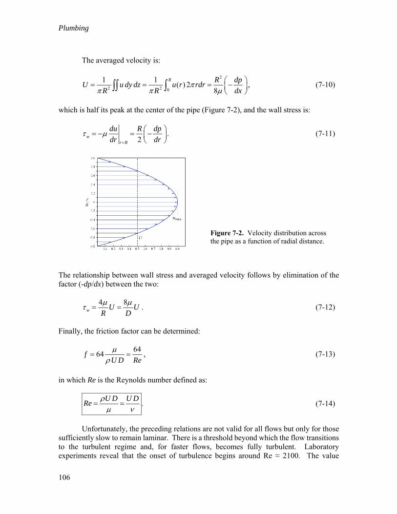
which is half its peak at the center of the pipe (Figure 7-2), and the wall stress is:

2w

r R

du R dp

dr dr

. (7-11)

Figure 7-2. Velocity distribution across the pipe as a function of radial distance.

The relationship between wall stress and averaged velocity follows by elimination of the factor (-dp/dx) between the two:

4 8

w U UR D

. (7-12)

Finally, the friction factor can be determined:

64

64fU D Re

, (7-13)

in which Re is the Reynolds number defined as:

U D U D

Re

. (7-14)

Unfortunately, the preceding relations are not valid for all flows but only for those sufficiently slow to remain laminar. There is a threshold beyond which the flow transitions to the turbulent regime and, for faster flows, becomes fully turbulent. Laboratory experiments reveal that the onset of turbulence begins around Re ≈ 2100. The value

Plumbing

107

remains imprecise because it depends on many details such as the manner by which the fluid is introduced at the entrance of the pipe and by which it is being gradually accelerated. 7-3. Turbulent flow in a pipe Beyond Re ≈ 2100 and up to Re ≈ 4000, there is a transition zone, in which the flow is relatively unstable, oscillating in places between laminar and turbulent regimes. For Re > 4000, the flow is no longer intermittent and is well established as a turbulent flow. In the turbulent regime, we know from Section 6-5 that the velocity profile in the vicinity of the wall is logarithmic. For a smooth wall, the velocity distribution with from the wall is given by (6-14a,b) as a function of the distance R–r from the wall:

2* ( )

( )u R r

u r

for *( )12

u R r

(7-15a)

* **

( )( ) ln 5.56

u u R ru r u

for *( )12

u R r

. (7-15b)

Toward the centerline line of the pipe, the logarithmic velocity profile from one side meets that from the opposite side, and the meeting of the two forms a cusp. Of course, no such a cusp exists in reality, and the velocity profile is smoothly varying around r = 0. Nevertheless, we assuming here as a first approximation that the flow is logarithmic all the way from the wall (thus neglecting the viscous sublayer) to the centerline (where we ignore the cusp), and we will adjust the result afterwards based on laboratory data. Using expression (7-15b) all the way from r = 0 to r = R, we estimate the mean velocity. After some algebra, we obtain:

* **2 0

1 3( ) 2 ln 5.56

2

R u RuU u r rdr u

R

. (7-16)

Since the turbulent stress is related to the friction velocity by 2

*w u , it follows that

2

2

*1 3ln 5.56

2 2

w

U

Du

. (7-17)

Note that this is an implicit relation since u*, which is the wall stress in disguise, occurs in the denominator on the right-hand side. In terms of the friction factor, this expression becomes:

Plumbing

108

22

88

1 3ln 5.56

4 2 2

wfU Re f

.

This is usually re-packaged for ease of calculations in terms of 1/ f :

1 1 1 3

ln 5.564 2 22 2

Re f

f

or, after performing the numerical evaluations with = 0.40,

10.88ln 0.89Re f

f . (7-18)

Based on laboratory data with smooth pipes, the coefficients should be adjusted as follows:

10.87 ln 0.80Re f

f . (7-19)

This adjustment makes up for the fact that we were quite approximate in our use of the velocity profile. For a rough wall, the roughness height z0 supersedes the viscosity as the factor in the logarithmic velocity profile, according to (6-13):

*

0

( ) lnu R r

u rz

. (7-20)

Assuming again that this is valid from wall to centerline, we deduce the average velocity:

*2 0

0

1 3( ) 2 ln

2

R u RU u r rdr

R z

, (7-21)

which we relate to the stress using 2

*w u :

2 2

2

0

3ln

2 2

w

U

Dz

, (7-22)

Plumbing

109

which is a purely quadratic relationship between stress and averaged velocity. In terms of the friction factor, this becomes:

2

2

0

8

3ln

2 2

fDz

,

which is independent of the Reynolds number and can be recast as:

0

11.94 0.88ln

D

zf

. (7-23)

The empirical relation obtained from laboratory data on rough pipes, to which we could compare (7-23) does not use the roughness height z0 as defined in Section 6-5 and which goes into the logarithmic profile, but uses the height of the averaged roughness element, denoted e and which is about 20 times as large z0. With z0 ≈ e/20, (7-23) becomes:

1

0.71 0.88lnD

ef

.

Adjustment of the numerical coefficients to fit laboratory data leads to:

1

1.14 0.87 lnD

ef

. (7-24)

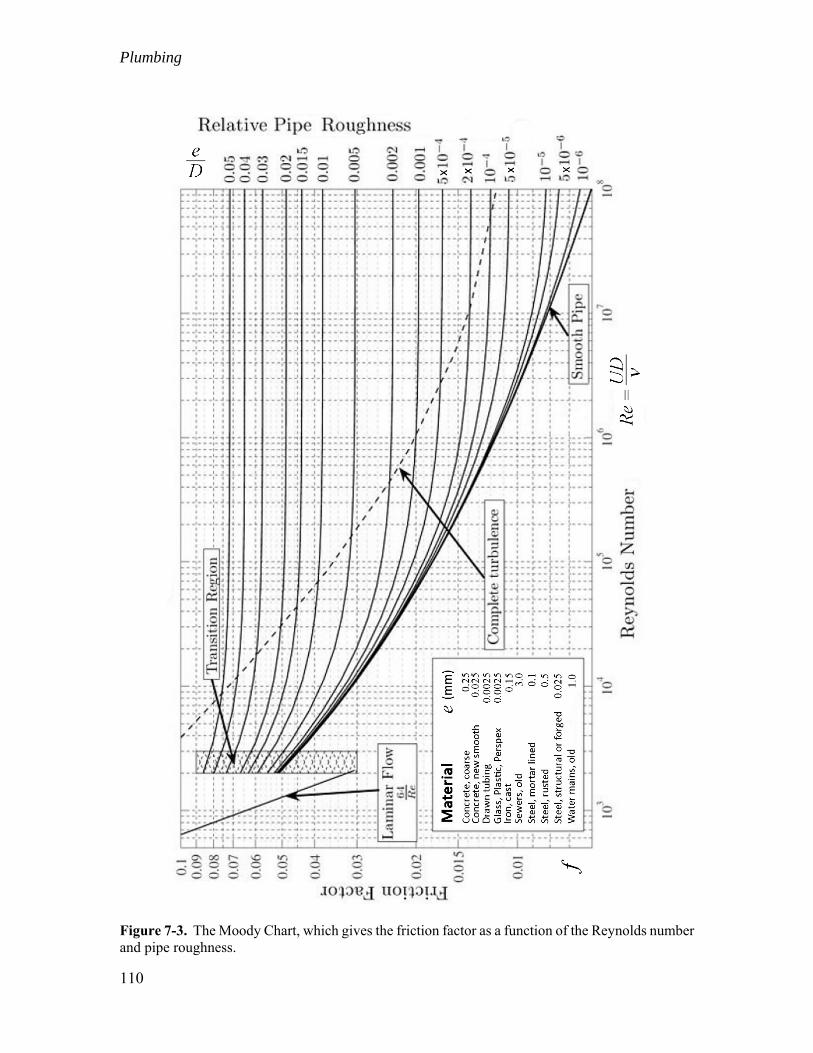
Assembling all the information, on laminar flow, turbulent flow in smooth pipes, and turbulent flow in rough pipes, we obtain the so-called Moody Chart, reproduced here as Figure 7-3. It provides the friction factor f as a function of the Reynolds number Re = UD/ of the flow, and the relative roughness e/D of the inner pipe wall. To avoid the reading of imprecise numbers from a graph or to automate calculations in a computer program, the following formulas are recommended:

For Re < 2100, use the laminar formula: 64

fRe

(7-25)

For 2100 < Re < 4000: Transitory and unstable situation to be avoided.

For 4000 < Re, use the so-called Colebrook-White formula that recapitulates both

turbulent cases:

1 9.29

1.14 0.87 lne

Df Re f

(7-26)

Plumbing

110

Figure 7-3. The Moody Chart, which gives the friction factor as a function of the Reynolds number and pipe roughness.

Plumbing

111

It is interesting to use the Moody Chart to the drinking from a straw to answer the question of how much sucking pressure is spent on overcoming gravity and how is spent on friction. For this, we set the following four variables (Figure 7-4): the inner diameter D of the straw, its length L, the elevation H from the surface of the beverage to the mouth, and the flow rate Q.

Figure 7-4. Drinking from a straw, with pertinent notation.

If the person drinks a cup-full of about 600 cm3 in 45 seconds, Q = 1.33 x 10-5 m3/s, and if the inner diameter of the straw is 8 mm, the averaged velocity of the beverage in the straw is U = (1.33 x 10-5 m3/s)/(5.03 x 10-5 m2) = 0.27 m/s. This makes the Reynolds number be about Re ≈ (0.27 m/s)(0.008 m)/(1.14 x 10-6 m2/s) = 1860, which falls in the laminar regime because it is less than 2100. Thus, the friction factor is f = 64/Re = 0.034. For a straw length of L = 24 cm, the frictional pressure drop according to (7-7) is:

2

3 2

2

0.034 (1000 kg/m )(0.27 m/s) (0.24 m)37.2 Pa .

2 (0.008 m)

f U Lp

D

In comparison, the pressure difference due to gravity over an elevation H = 16 cm is: 3 2(1000 kg/m )(9.81 m/s )(0.16 m) 1570 Pap gH . Thus, we see that only 2% of the sucking pressure to be applied by the mouth to the straw is to overcome friction, with the remaining 98% being needed to overcome gravity. A second application is the estimation of the power needed to flow municipal drinking water over 1km of underground steel piping. (to be continued)

Plumbing

112

7-4. Water hammer Have you ever heard a loud clang or clatter coming from the plumbing system of the building in which you are, like a hammering noise? This is called water hammer, a phenomenon caused by a sudden variation in pipe flow, such as upon the quick closing of a faucet or valve in a pipe with fast moving water. The sudden halt of fast moving water generates a shock wave that triggers compressibility effects and travels across the system back and forth until its energy dissipates. The nature of the compressibility is two-fold; there is compressibility of the water itself (weak but not zero) as well as elasticity in the pipe material (widening and shrinking of its cross-section). A compressibility wave is a sound wave because it generates frequencies in our audible range, which we perceive as noise. Because it severely stresses the pipes and also because of its unwelcome noise, water hammer is something to be avoided. The remedy is to place somewhere along the system an air chamber that can accommodate the compressibility effects in gentle fashion. The physics of water hammer can be described relatively simply by means of a one-dimensional model retaining only the axial variability of the flow in the downstream direction and ignoring variations across the pipe (Mohamed Ghidaoui et al., 2005). For this, we can start by integrating the equations of motion in the two transverse directions in order to retain only the axial direction and time, but it is tricky because of the distorting pipe geometry. It is easier as well as more intuitive to return to the basic principles of mass conservation and momentum balance. We define the along-pipe direction as the x-axis, A as the cross-sectional area of the pipe, and U as the averaged flow velocity through A. The mass balance is relatively straightforward to state. The accumulation over time of mass dm = dV=Adx in the stretch of pipe from position x to x+dx is equal to the mass flux AU entering at x minus that exiting at position x+dx:

( )

x x dx

d AdxAU AU

dt

.

In the limit dx → 0, this can be recast as

1 ( )

0d A U

A dt x

, (7-27)

in which / / /d dt t U x stands for the material derivative. Both density and cross-sectional area A change with pressure p in the pipe. We are led to define:

2

1 d dA

c dp A dp

. (7-28)

Plumbing

113

The first term arises from the compressibility of the water whereas the second term from that of the pipe. So defined, the (positive) quantity c happens to be the sound speed of the water plus pipe wall combination. Because water is weakly compressible and the pipe material weakly elastic, the quantity 1/c2 is tiny, which makes c be a large speed, much larger than the water velocity: c U . (7-29) In practice, the sound speed ranges from 100 to 1400 m/s depending on the water temperature and especially the elasticity of the pipes, with the higher values being most likely, while the flow velocity will never exceed 10 m/s, with a few meters per second being most common (Ghidaoui et al., 2005). Another way of stating (7-29) is that the water flow in the pipe is very subsonic (Mach number << 1). With definition (7-28) becomes:

2

10

dp U

c dt x

. (7-30)

The momentum balance likewise follows. The accumulation over time of momentum (dm)U = (dV)U=AUdx in the stretch of pipe from position x to x+dx is equal to the momentum flux (AU)U entering at x minus that exiting at position x+dx plus the sum for pushing forces and minus the braking forces:

2 2( )( ) ( ) wx x dxx x dx

d AU dx dzAU AU pA pA dm g Ddx

dt dx

,

in which p is the pressure, g the gravitational acceleration, dz/dx the slope of the pipe axis with respect to the horizontal (positive upward), and w the frictional wall stress against the inner pipe surface Ddx. Doing the same algebra as for the mass conservation equation, we can recast this equation as1

( )

w

d AU U p dzAU A g A D

dt x x dx

.

Then using (7-27) and after division by A, it can be reduced to:

1 wdU p dz D

gdt x dx A

. (7-31)

Equations (7-30)-(7-31) can be simplified by introducing the piezometric head h, defined differentially as

1 Delicate point: The difference

x x dxpA pA

in the limit dx → 0 is /A p x rather than ( ) /pA x because

of the axial contribution of the pressure on the slanted pipe wall.

Plumbing

114

dp

dh dzg

, (7-32)

which is a way of capturing the pressure minus its hydrostatic component in terms of a height. With (7-6) to express the ratio w/ in terms of the flow velocity U, (7-32) to replace p in terms of h, and finally A = D2/4, Equations (7-30) and (7-31) reduce to:

2

0dh dz c U

dt dt g x

(7-33a)

2

2

dU h fg U

dt x D

, (7-33b)

where f is the friction factor encountered at the end of Section 7-1. We now have a complete set of equations since (7-33a,b) form a 2-by-2 set of differential equations for the two remaining variables U and h, each function of x and t. A last and major simplification can be made by taking advantage of the fact that the flow velocity U and therefore also the vertical velocity w = dz/dt are both much slower than the sound speed c, as already noted in (7-29). With very little approximation, the material derivative reduces to its first term, the partial derivative with respect to time, and we obtain:

2

0h c U

t g x

(7-34a)

2

2

U h fg U

t x D

. (7-34b)

The solution in the frictional case is fairly complicated because of the nonlinearity of the U2 term (and indirectly also from the fact that, if the pipe is not too rough, f varies with the Reynolds number and therefore U), but for a moderate length, friction may be neglected. The solution is then a simple sine wave:

( , ) cosx

h x t H tc

, ( , ) cos

gH xU x t t

c c

(7-35)

with amplitude H and angular frequency . The wave propagates along the pipe at speed dx/dt = c because the phase remains unchanged at that speed. 7-5. What happens when the pipe changes The preceding considerations restricted the attention to pipes with uniform diameter D; they also ignored any possible bend, elbow or tee along the pipe. In a sharp curve, the

Plumbing

115

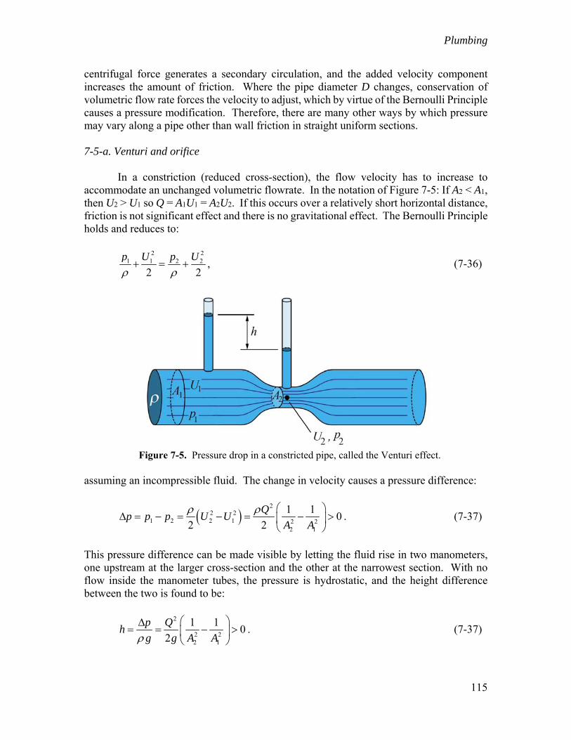
centrifugal force generates a secondary circulation, and the added velocity component increases the amount of friction. Where the pipe diameter D changes, conservation of volumetric flow rate forces the velocity to adjust, which by virtue of the Bernoulli Principle causes a pressure modification. Therefore, there are many other ways by which pressure may vary along a pipe other than wall friction in straight uniform sections. 7-5-a. Venturi and orifice In a constriction (reduced cross-section), the flow velocity has to increase to accommodate an unchanged volumetric flowrate. In the notation of Figure 7-5: If A2 < A1, then U2 > U1 so Q = A1U1 = A2U2. If this occurs over a relatively short horizontal distance, friction is not significant effect and there is no gravitational effect. The Bernoulli Principle holds and reduces to:

2 2

1 1 2 2

2 2

p U p U

, (7-36)

Figure 7-5. Pressure drop in a constricted pipe, called the Venturi effect.

assuming an incompressible fluid. The change in velocity causes a pressure difference:

2

2 21 2 2 1 2 2

2 1

1 10

2 2

Qp p p U U

A A

. (7-37)

This pressure difference can be made visible by letting the fluid rise in two manometers, one upstream at the larger cross-section and the other at the narrowest section. With no flow inside the manometer tubes, the pressure is hydrostatic, and the height difference between the two is found to be:

2

2 22 1

1 10

2

p Qh

g g A A

. (7-37)

Plumbing

116

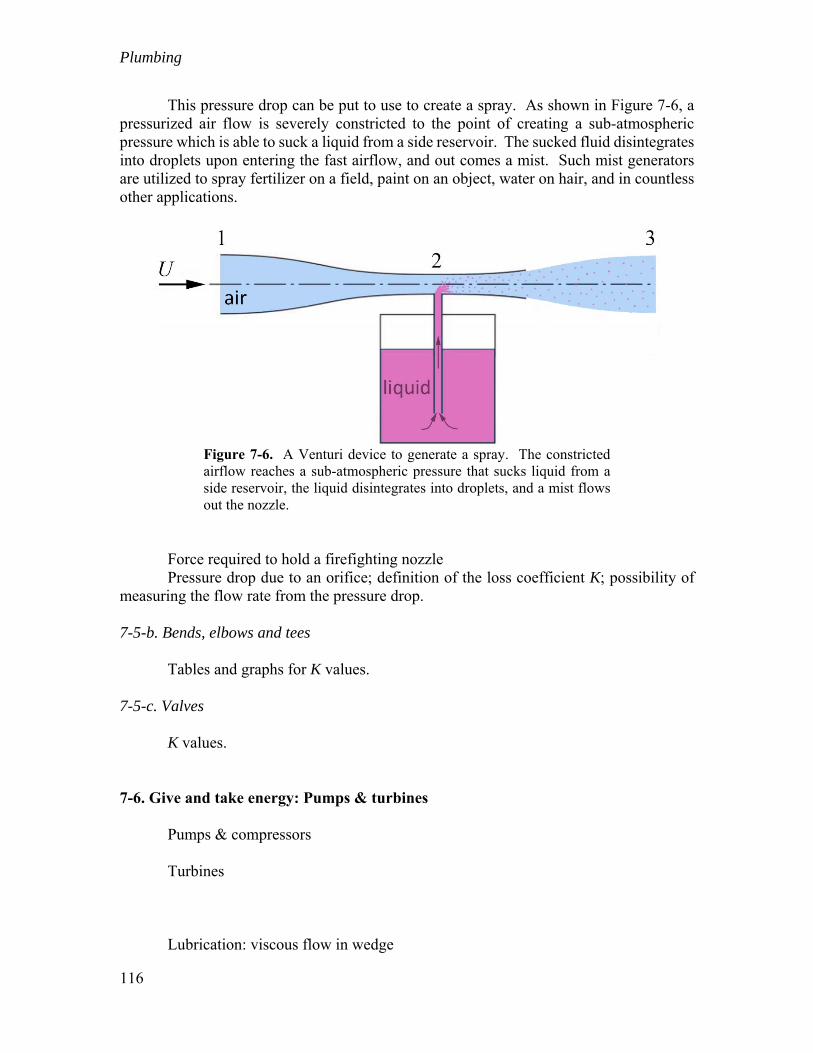
This pressure drop can be put to use to create a spray. As shown in Figure 7-6, a pressurized air flow is severely constricted to the point of creating a sub-atmospheric pressure which is able to suck a liquid from a side reservoir. The sucked fluid disintegrates into droplets upon entering the fast airflow, and out comes a mist. Such mist generators are utilized to spray fertilizer on a field, paint on an object, water on hair, and in countless other applications.

Figure 7-6. A Venturi device to generate a spray. The constricted airflow reaches a sub-atmospheric pressure that sucks liquid from a side reservoir, the liquid disintegrates into droplets, and a mist flows out the nozzle.

Force required to hold a firefighting nozzle Pressure drop due to an orifice; definition of the loss coefficient K; possibility of measuring the flow rate from the pressure drop. 7-5-b. Bends, elbows and tees Tables and graphs for K values. 7-5-c. Valves K values. 7-6. Give and take energy: Pumps & turbines Pumps & compressors Turbines Lubrication: viscous flow in wedge

Plumbing

117

Thought problems 7-T-1. Question 7-T-2. Question 7-T-3. In the application to the drinking with a straw (Figure 7-4), the elevation H was

taken from the surface of the beverage to the mouth. Why not from the bottom tip of the straw?

Quantitative Exercises 7-Q-1. Question 7-Q-2. Question 7-Q-3. Question