166

Chapter 7

Addressing The Problem

7.1 Introduction

The goal of this thesis is to develop a classifier which discriminates between

surfaces on the basis of their visual appearance. The development of such a classifier is

described in Chapter 5. However, using the models developed in the earlier chapters it is

shown in Chapter 6 that the direction of illumination is a critical factor in the

performance of the classifier. This chapter will review a range of candidate techniques

on which a classifier that is robust to tilt variations may be based. One technique will be

selected for further investigation in the next chapter.

Having observed the effect, we now consider some techniques aimed at reducing

tilt induced misclassification error. Chantler proposed four schemes [Chantler94], we

will begin by discussing all four and evaluating the three which we believe most

appropriate to the terms of this thesis. Since we wish to classify textures on the basis of

their surface properties, we then proceed to review the field of shape from shading.

Finally, we propose a novel scheme which uses a model based technique to overcome the

problem of tilt induced classifier failure.

7.2 Review of Chantler’s Feature Space Proposals

In [Chantler94] Chantler proposes four techniques for conferring tilt-robustness on a

classifier:

(i) a single classification rule obtained by training over the tilt range,

(ii) a series of rules indexed by tilt,

(iii) a segmentation based technique, and

167

(iv) a filter based technique designed to reverse the directional effects of

illumination.

The first three techniques operate in feature space, whereas the last pre-processes the

image before feature extraction. In his thesis, Chantler chose to investigate only the last

option. In this work we will discuss each and investigate those which are relevant to this

thesis.

7.2.1 Multiple Training Samples

Chantler’s first proposal is to train the classifier over the range of illuminant

conditions it is likely to encounter. He notes that the increased variance of each class

may reduce classification accuracy and pursues the idea no further. We reconsider the

scheme in the following terms:

In Chapter 5 we introduced a discriminant which classified a pixel, with feature

vector F, as having label �l on the criterion shown below:

[ ]�( )arg max

( ( ))ll

p li

l iiF F

F=

where p ll iiF

F( ) is the probability density function of feature F, given that a pixel

belongs to class i.

In Chapter 6 we showed that the probability density function of vector F,

p li( )F , is a function of the illuminant tilt. We treat tilt angle as a random variable,

randomly distributed between 0 and 2π, and describe using the joint pdf:

p li( , )F τ

Chantler's proposal attempts to classify pixels on the basis of an approximation to

the marginal density of p. The marginal distribution will be the integral of the joint

density over tilt (7.2.1a), assuming the illuminant tilt angle is drawn from a uniform

distribution, and the feature distributions vary continuously. This can be approximated

by the summation of a finite number of sample distributions (7.2.1b).

K l p l di i( ) ( , )F F= ∫ τ τ

π

0

(7.2.1a)

168

K p f li’( ) ( , )==∑τ

πτ

0

F (7.2.1b)

Where classification is made on the basis of:

[ ]�( )arg max

( ( ))ll

K li

C iiF F

F=

The probability function Ki(p) will occupy at least an equal, or more probably, a

larger volume of feature space than any of its component (tilt conditional) density

functions. There will consequently be a greater degree of overlap between clusters of

different classes. The success of the classifier is dependent on the degree of tilt induced

cluster movement being small relative to the distribution separation. In Figure 7.2.1 we

plot the feature means derived from filters oriented at 0° and 90° which have been

applied to the exemplar textures: Rock and Striate.

0

10

20

30

40

50

60

70

0 10 20 30 40 50 60 70 80 90 100 110 120 130 140 150 160 170 180

Tilt Angle (°)

Fea

ture

Val

ue

Rock

Striate

0

5

10

15

20

25

30

35

40

45

50

0 10 20 30 40 50 60 70 80 90 100 110 120 130 140 150 160 170 180

Tilt Angle (°)

Fea

ture

Val

ue

RockStriate

Figure 7.2.1 Feature means for Rock and Striate textures calulated from F25 filters

oriented at 0° and 90°.

In Figure 7.2.1, it is shown that the assumption that cluster separation is large

relative to cluster movement is not reasonable for the texture features measured on the

Rock and Striate textures. While the clusters may or may not overlap at a given tilt, the

movement of the means with tilt, in both cases, clearly show that it is not possible to set

a single threshold to discriminate between the textures throughout the tilt range.

Although this technique is not appropriate in the above case, we have not ruled

out the possibility that it may be effective for data sets which are well separated in

feature space. While the technique is not universally applicable to the tilt problem, its

simplicity of implementation makes it worthy of investigation for a given data set. We

also conclude from the inadequacy of a single threshold that a priori knowledge of the

169

illuminant tilt angle is a necessary condition for the illuminant invariant classification of

rough surfaces. This leads us to Chantler’s second proposal.

7.2.2 Multiple Discriminants

Chantler’s second proposal uses multiple training samples captured under various

illumination conditions to build a library of discriminant functions which can then be

indexed by tilt angle. Any practical system will have a finite number of training samples.

In the context of the schemes considered later in this chapter, we limit ourselves to three

training images.

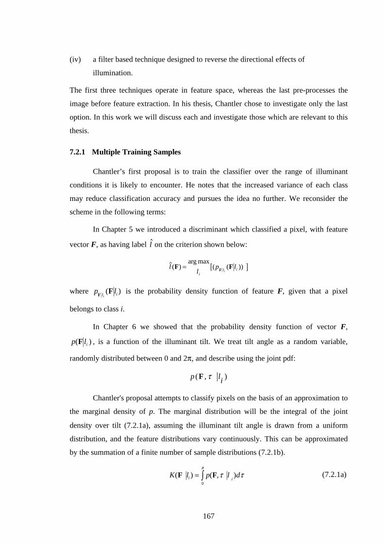
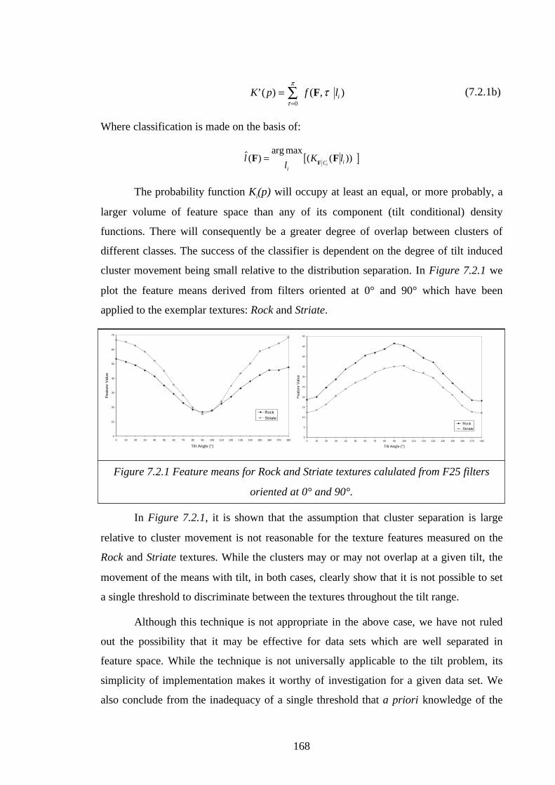
We conducted experiments on the Anaglypta and both the Stone montages, in

each case using three discriminants, developed at 0°,90° and 180°, switching between

discriminants at 50° and 140° respectively.

Anaglypta Montage

0

10

20

30

40

50

60

70

80

0 10

20

30

40

50

60

70

80

90

10

0

11

0

12

0

13

0

14

0

15

0

16

0

17

0

18

0

Tilt Angle (°)

Mis

clas

sific

atio

n (%

)

Figure 7.2.2 The use of three discriminants with the anaglypta montage.

Stones 1 Montage

0

10

20

30

40

50

60

70

80

0 10 20 30 40 50 60 70 80 90 100 110 120 130 140 150 160 170 180

Tilt Angle (°)

Mis

clas

sific

atio

n R

ate

(%)

Stones 2 Montage

0

10

20

30

40

50

60

70

0 10 20 30 40 50 60 70 80 90 100 110 120 130 140 150 160 170 180

Tilt Angle (°)

Mis

cla

ssifi

catio

n (

%)

Figure 7.2.3 The use of three discriminants with Stone montages.

170

As we might expect, the misclassification graph has minima at 0°,90° and 180°.

However, the majority of intermediate points show an unacceptably high

misclassification rate. The speed with which classification errors increase as we move

away from the training angle also suggests that the necessary interval between training

samples is so small, certainly less than 20°, as to be uneconomical for a practical

classification system. This immediately suggests an interpolative scheme, however non-

linearities in both the imaging and the classification processes make this problematic.

Later in this chapter we will propose a technique that is a derivative of this scheme, but

which operates in image, rather than feature space, circumventing the problems of non-

linearity.

7.2.3 Segmentation/Classification

The rationale for this scheme is that since the problem is caused by movement of

clusters across discriminant boundaries an appropriate strategy is to track the clusters

using cluster analysis techniques. The postulated clusters then may be identified as

belonging to an a priori defined class at a higher level in the image understanding

hierarchy. Identification at this level would be carried out by some feature measure

(Chantler suggests features based on the power spectra) which for reasons of

computational cost, or the requirement for homogenous regions of data, could not be

effectively integrated into the lower levels. We note that cluster analysis is being used as

a segmentation tool, and is therefore interchangeable with other segmentation techniques,

such as edge-based or region growing approaches. This scheme is effectively an

unsupervised technique, and consequently outwith the terms of this thesis. We do not

investigate it further.

7.3 Chantler’s Filters

While Chantler proposed four techniques he selected only one for further

investigation. Unlike the earlier techniques which seek to deal with the feature space

effects of tilt variation, this technique is proactive, and seeks to remove, or at least

mitigate the effects of tilt before features are extracted.

171

7.3.1 Review

Chantler proposed and evaluated a system of filters to reduce the effect of tilt

effects on the classification of texture [Chantler94]. After verifying Kube’s work on real

textures, Chantler used this model as the basis on which he could develop a frequency

domain technique to remove the directional effect introduced by illumination—treating

the problem essentially as one of inverse filtering. In this section we consider four issues

that arise from this scheme.

• Linearity: the filters are subject to the restrictions on surface type and lighting

conditions considered in Chapter 3. Chantler attempted to model the effects of non-

linearity by adding an empirical term, b, to form his F1 filter class (7.3.1a). In effect

treating the unwanted signal components as additive white noise.

Hm Cos bF1

1( , )( )

ω θ θ τ= − + (7.3.1a)

where

m and b are empirically derived coefficients.

• Frequency dependency: if we attempt to fit the F1 model to radial plots taken at

different frequencies we find a significant radial frequency dependency in both terms.

This led Chantler to develop the modified F2 model, where the second order parameters

are estimated in a two stage process: first, radial plots are taken for overlapping

frequency ranges, the m and b parameters are fitted to each using least squares; second a

linear least squares model is fitted to each parameter as a function of frequency.

Hm Cos b

( , )( ) ( ) ( )

ω θ ω θ τ ω=− +

1 (7.3.1b)

• Directionality: as the estimation process can only be applied to isotropic or near

isotropic textures, it assumes that directional textures, for which parameters cannot be

estimated, will be similarly affected by changes in tilt. In Chapter 3 it was shown that

rough directional surfaces do exhibit behaviour incompatible with Kube's model. In

combination with the linearity restrictions this forms a significant limit to the utility of

the scheme. The degree of restriction is illustrated by the fact that the isotropy condition,

strictly applied, would rule out all the test montages.

172

• Optimality: The work reported in Chapter 3 was based on the performance of a filter

which was optimal for a particular texture. In a classification problem, we must accept

the fact that any general filter will be sub-optimal for each texture. If we reconsider the

frequency variation of model parameters with frequency for different textures we see that

there is a wide variation from texture to texture. Chantler tackled this problem by

averaging the model parameters for each texture. Whether the resulting sub-optimal filter

will be sufficiently effective will depend on the similarity of the textures. This

interdependency limits the generality of any experimental results obtained.

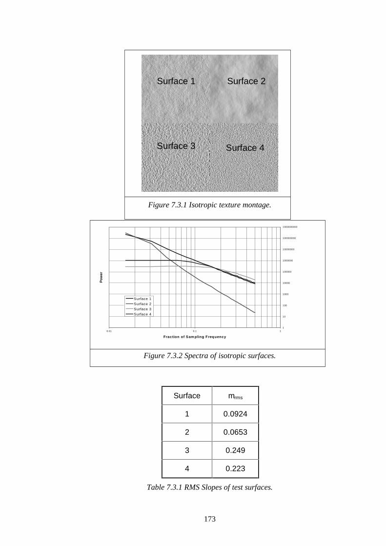
In order to address these issues, prior to an evaluation of the technique, a new set of

synthetic textures Figure 7.3.1 is introduced.

• Linearity: in chapter 3 we concluded that the major factor affecting how well a linear

model describes rendering is the rms slope of the surface. The rms slopes of the synthetic

surfaces are shown in Table 7.3.1.

• Directionality: the requirement for isotropic surfaces is satisfied by using Malvaney

and fractal surface models.

• Frequency dependency: The synthetic textures can be used to gauge the effect of

frequency dependency in the optimal parameter values. The distinct radial frequency

characteristics of the fractal and Mulvaney models provides one point of comparison.

The fractal surfaces (1 and 2) differ in their roll-off rates, β=3.0 and 4.5 respectively.

The Mulvaney surfaces differ in the cut-off frequency at which the transition between

white noise and fractal roll-off occurs.

• Optimality: The issue of optimality is accomodated into the evaluation in two steps.

Firstly, experiments are carried out on a texture by texture basis. In each case the filter is

designed purely for that texture. In the second stage the filter parameters of the texture

specific filters are averaged to produce a general filter which is applied to all the textures

in the montage.

The spectra and rms slope of the surfaces are shown in Figure 7.3.2 and respectively.

173

Figure 7.3.1 Isotropic texture montage.

1

10

100

1000

10000

100000

1000000

10000000

100000000

1000000000

0.01 0.1 1

Fraction of Sam pling F requency

Po

wer

Surface 1

Surface 2

Surface 3

Surface 4

Figure 7.3.2 Spectra of isotropic surfaces.

Surface mrms

1 0.0924

2 0.0653

3 0.249

4 0.223

Table 7.3.1 RMS Slopes of test surfaces.

Surface 1 Surface 2

Surface 3 Surface 4

174

7.3.2 A Texture Specific Filter

In the last section it was concluded that a significant limitation of the technique

would be the requirement for it to generalise, i.e. to operate effectively for a range of

textures. Our assessment of the algorithm proceeds in two stages. In this section we

ignore the question of generality and test the form of the filter—each texture is processed

by a filter designed specially for that surface. In the next section the impact on

performance of the general filter is assessed. This experiment represents a more realistic

test of the algorithm. By resolving our assessment into two distinct stages we believe we

will gain a better understanding of the technique's performance.

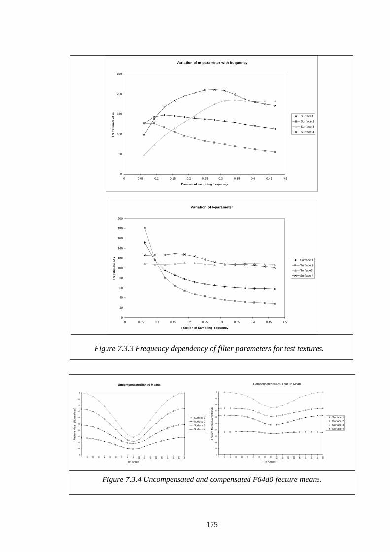
We begin by estimating the model parameters for each texture in the test set. This

is done by splitting the power spectrum of each texture into fourteen radial frequency

bands.The polar distribution of signal magnitude for each band is measured and a curve

of the form mcos(θ-τ)+b is then fitted to the polar plot using least squares. The m and b

parameters plotted against frequency in Figure 7.3.3. For both parameters the family of

parameter curves can immediately be split into two groups which correspond to whether

the surface is fractal (surfaces 1&2) or of the Mulvanney type (surfaces 3&4). The

fractal textures exhibit a gradual decline in the value of the m-parameter with frequency,

whereas for the Mulvanney surfaces the parameter actually increases before saturating.

In the case of the b-parameter the Mulvanney surfaces are largely independent of

frequency while the fractals show a significant drop with frequency. We therefore

conclude that the form of the filter is a function of the surface type.

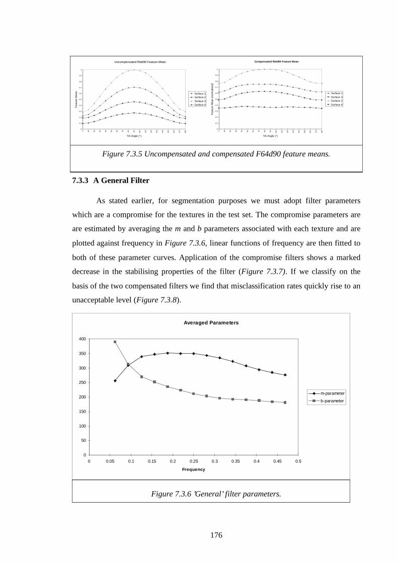
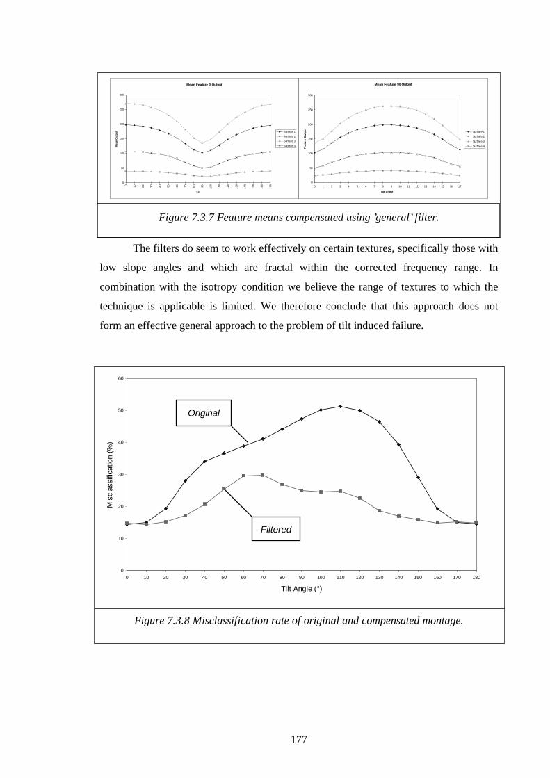
In our first application of the filters we postpone the issue of optimality and treat

each texture independently. The F2 model is fitted to and applied to each texture. This

involves fitting linear functions of frequency to both the parameter curves. We then

examine the output of the 0 and 90° features of the f64 filter set, which is concentrated in

the model's linear region (ω<0.25ωs). In all the compensated cases the variation of

feature output with tilt angle is much flatter, i.e. more stable than the uncompensated

outputs (Figure 7.3.4 and Figure 7.3.5). However, we note the decrease in the

effectiveness of the filters with the rougher surfaces. Even with F2 filters optimised to a

particular texture the effect has not been eliminated.

175

Variation of m-parameter with frequency

0

50

100

150

200

250

0 0.05 0.1 0.15 0.2 0.25 0.3 0.35 0.4 0.45 0.5

Fraction of sampling frequency

LS

Est

imat

e o

f m Surface1

Surface 2

Surface 3

Surface 4

Variation of b-parameter

0

20

40

60

80

100

120

140

160

180

200

0 0.05 0.1 0.15 0.2 0.25 0.3 0.35 0.4 0.45 0.5

Fraction of Sampling Frequency

LS

est

imat

e o

f b Surface 1

Surface 2

Surface3

Surface 4

Figure 7.3.3 Frequency dependency of filter parameters for test textures.

Uncompensated f64d0 Means

0

0.1

0.2

0.3

0.4

0.5

0.6

0.7

0.8

0.9

1

0 10 20 30 40 50 60 70 80 90 100

110

120

130

140

150

160

170

180

Tilt Angle

Fea

ture

Mea

n (N

orm

alis

ed)

Surface 1Surface 2Surface 3Surface 4

Compensated f64d0 Feature Mean

0

0.1

0.2

0.3

0.4

0.5

0.6

0.7

0.8

0.9

1

0 10 20 30 40 50 60 70 80 90 100

110

120

130

140

150

160

170

180

Ti lt Angle (°)

Fea

ture

Mea

n (N

orm

alis

ed)

Surface 1Surface 2Surface 3Surface 4

Figure 7.3.4 Uncompensated and compensated F64d0 feature means.

176

Uncompensated f64d90 Feature Mean

0

0.1

0.2

0.3

0.4

0.5

0.6

0.7

0.8

0.9

1

0 10 20 30 40 50 60 70 80 90 100

110

120

130

140

150

160

170

180

Tilt Angle (°)

Fea

ture

Mea

n

Surface 1Surface 2

Surface 3Surface 4

Compensated f64d90 Feature Mean

0

0.1

0.2

0.3

0.4

0.5

0.6

0.7

0.8

0.9

1

0 10 20 30 40 50 60 70 80 90 100

110

120

130

140

150

160

170

180

Tilt Angle (°)

Fea

ture

Mea

n (n

orm

alis

ed)

Surface 1

Surface 3Surface 2

Surface 4

Figure 7.3.5 Uncompensated and compensated F64d90 feature means.

7.3.3 A General Filter

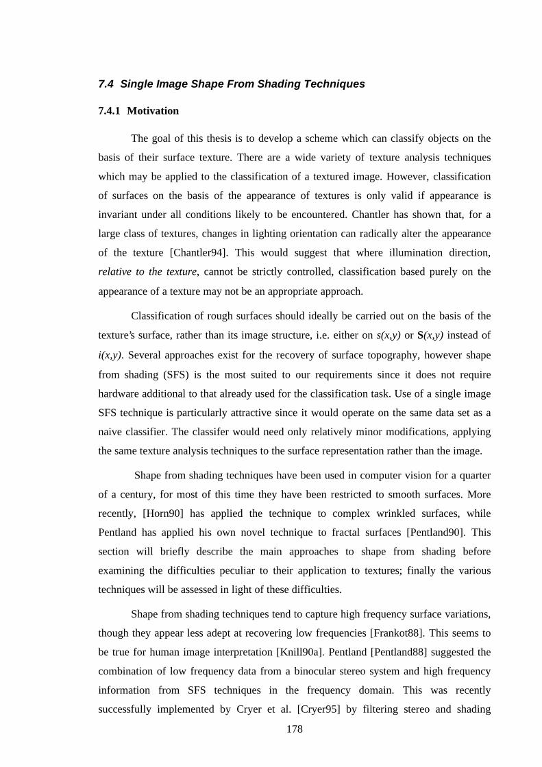
As stated earlier, for segmentation purposes we must adopt filter parameters

which are a compromise for the textures in the test set. The compromise parameters are

are estimated by averaging the m and b parameters associated with each texture and are

plotted against frequency in Figure 7.3.6, linear functions of frequency are then fitted to

both of these parameter curves. Application of the compromise filters shows a marked

decrease in the stabilising properties of the filter (Figure 7.3.7). If we classify on the

basis of the two compensated filters we find that misclassification rates quickly rise to an

unacceptable level (Figure 7.3.8).

Averaged Parameters

0

50

100

150

200

250

300

350

400

0 0.05 0.1 0.15 0.2 0.25 0.3 0.35 0.4 0.45 0.5

Frequency

m-parameter

b-parameter

Figure 7.3.6 ’General’ filter parameters.

177

Mean Feature 0 Output

0

50

100

150

200

250

300

0

10

20

30

40

50

60

70

80

90

10

0

11

0

12

0

13

0

14

0

15

0

16

0

17

0

Tilt

Mea

n O

utpu

t Surface 1

Surface 2

Surface 3

Surface 4

Mean Feature 90 Output

0

50

100

150

200

250

300

0 1 2 3 4 5 6 7 8 9 10 11 12 13 14 15 16 17

Tilt Angle

Fea

ture

Ou

tpu

t

Surface 1

Surface 2

Surface 3

Surface 4

Figure 7.3.7 Feature means compensated using ’general’ filter.

The filters do seem to work effectively on certain textures, specifically those with

low slope angles and which are fractal within the corrected frequency range. In

combination with the isotropy condition we believe the range of textures to which the

technique is applicable is limited. We therefore conclude that this approach does not

form an effective general approach to the problem of tilt induced failure.

0

10

20

30

40

50

60

0 10 20 30 40 50 60 70 80 90 100 110 120 130 140 150 160 170 180

Tilt Angle (°)

Mis

clas

sific

atio

n (%

)

Filtered

Original

Figure 7.3.8 Misclassification rate of original and compensated montage.

Filtered

Original

178

7.4 Single Image Shape From Shading Techniques

7.4.1 Motivation

The goal of this thesis is to develop a scheme which can classify objects on the

basis of their surface texture. There are a wide variety of texture analysis techniques

which may be applied to the classification of a textured image. However, classification

of surfaces on the basis of the appearance of textures is only valid if appearance is

invariant under all conditions likely to be encountered. Chantler has shown that, for a

large class of textures, changes in lighting orientation can radically alter the appearance

of the texture [Chantler94]. This would suggest that where illumination direction,

relative to the texture, cannot be strictly controlled, classification based purely on the

appearance of a texture may not be an appropriate approach.

Classification of rough surfaces should ideally be carried out on the basis of the

texture’s surface, rather than its image structure, i.e. either on s(x,y) or S(x,y) instead of

i(x,y). Several approaches exist for the recovery of surface topography, however shape

from shading (SFS) is the most suited to our requirements since it does not require

hardware additional to that already used for the classification task. Use of a single image

SFS technique is particularly attractive since it would operate on the same data set as a

naive classifier. The classifer would need only relatively minor modifications, applying

the same texture analysis techniques to the surface representation rather than the image.

Shape from shading techniques have been used in computer vision for a quarter

of a century, for most of this time they have been restricted to smooth surfaces. More

recently, [Horn90] has applied the technique to complex wrinkled surfaces, while

Pentland has applied his own novel technique to fractal surfaces [Pentland90]. This

section will briefly describe the main approaches to shape from shading before

examining the difficulties peculiar to their application to textures; finally the various

techniques will be assessed in light of these difficulties.

Shape from shading techniques tend to capture high frequency surface variations,

though they appear less adept at recovering low frequencies [Frankot88]. This seems to

be true for human image interpretation [Knill90a]. Pentland [Pentland88] suggested the

combination of low frequency data from a binocular stereo system and high frequency

information from SFS techniques in the frequency domain. This was recently

successfully implemented by Cryer et al. [Cryer95] by filtering stereo and shading

179

derived depth maps with low pass and high pass filters respectively. Since we are

concerned with textures, we are principally interested in the higher frequencies; shape

from shading therefore seems to be a promising approach.

7.4.2 Shape From Shading

Introduction

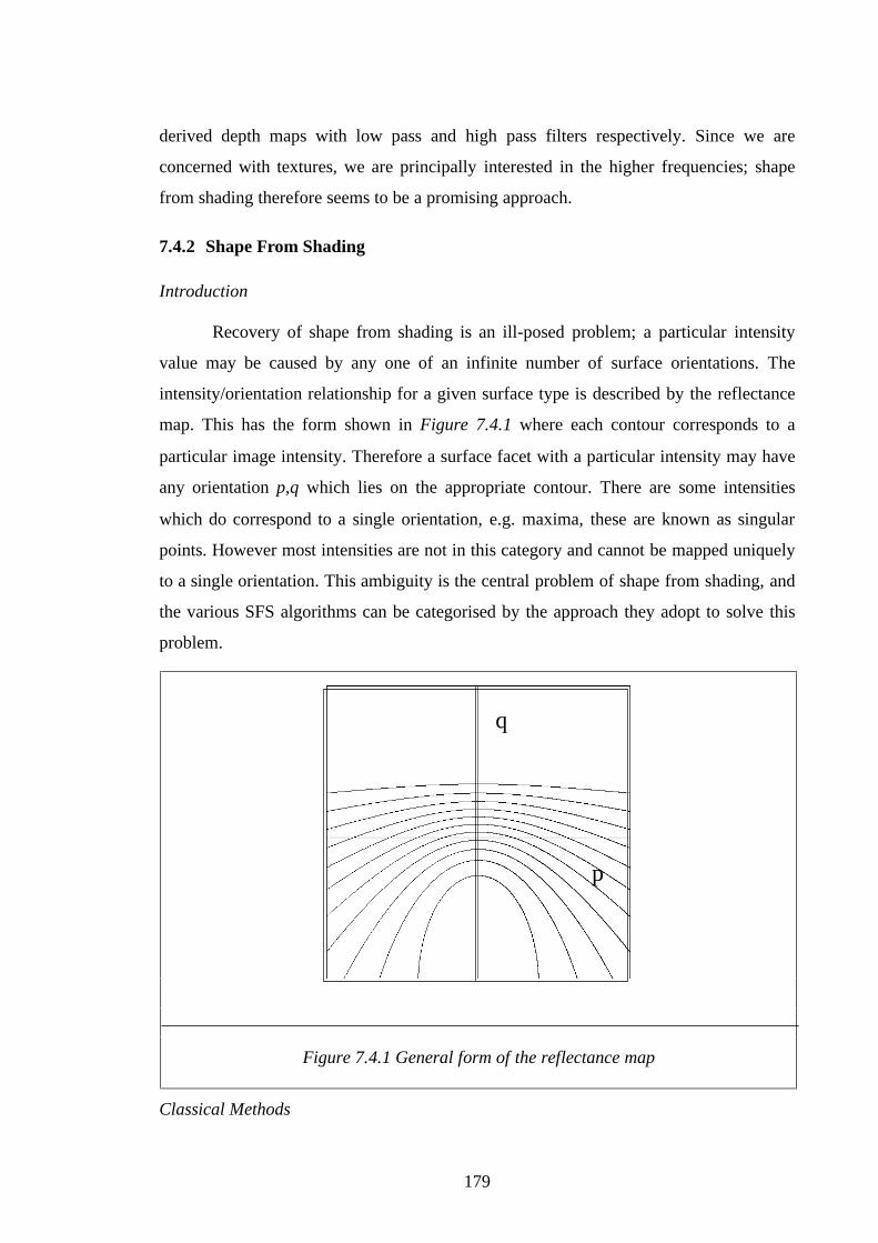
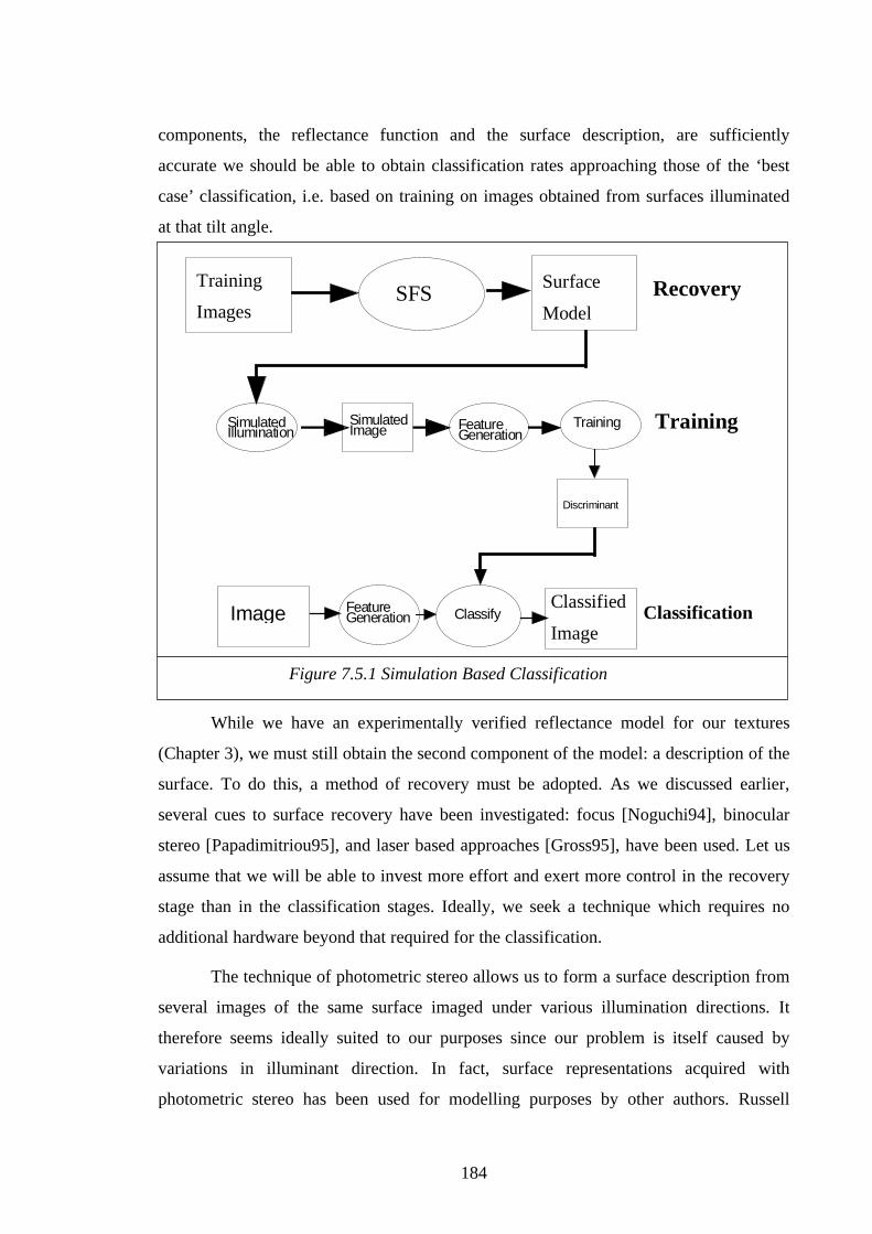
Recovery of shape from shading is an ill-posed problem; a particular intensity

value may be caused by any one of an infinite number of surface orientations. The

intensity/orientation relationship for a given surface type is described by the reflectance

map. This has the form shown in Figure 7.4.1 where each contour corresponds to a

particular image intensity. Therefore a surface facet with a particular intensity may have

any orientation p,q which lies on the appropriate contour. There are some intensities

which do correspond to a single orientation, e.g. maxima, these are known as singular

points. However most intensities are not in this category and cannot be mapped uniquely

to a single orientation. This ambiguity is the central problem of shape from shading, and

the various SFS algorithms can be categorised by the approach they adopt to solve this

problem.

Classical Methods

q

p

Figure 7.4.1 General form of the reflectance map

180

The first attempt to solve the shape from shading problem was proposed by Horn

[Horn70]. This treated the problem as that of solving a first order non-linear partial

differential equation. Proceeding from a singular point the equation was solved to give

characteristic curves of known orientation which were then grown to give the

orientations of the entire surface. This technique has several difficulties: it has not been

amenable to computer implementation, it is sensitive to measurement noise, and the areas

grown from characteristic strips do not always merge well. This technique has largely

been superceded by iterative schemes.

Iterative Techniques

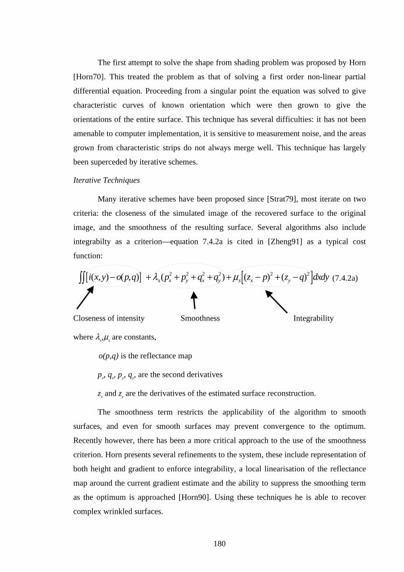
Many iterative schemes have been proposed since [Strat79], most iterate on two

criteria: the closeness of the simulated image of the recovered surface to the original

image, and the smoothness of the resulting surface. Several algorithms also include

integrabilty as a criterion—equation 7.4.2a is cited in [Zheng91] as a typical cost

function:

[ ] [ ]i x y o p q p p q q z p z q dxdys x y x y s x y( , ) ( , ) ( ) ( ) ( )− + + + + + − + −∫∫ λ μ2 2 2 2 2 2 (7.4.2a)

Closeness of intensity Smoothness Integrability

where λs,μs are constants,

o(p,q) is the reflectance map

px, qx, py, qy, are the second derivatives

zx and zy are the derivatives of the estimated surface reconstruction.

The smoothness term restricts the applicability of the algorithm to smooth

surfaces, and even for smooth surfaces may prevent convergence to the optimum.

Recently however, there has been a more critical approach to the use of the smoothness

criterion. Horn presents several refinements to the system, these include representation of

both height and gradient to enforce integrability, a local linearisation of the reflectance

map around the current gradient estimate and the ability to suppress the smoothing term

as the optimum is approached [Horn90]. Using these techniques he is able to recover

complex wrinkled surfaces.

181

Zheng and Chellapa have pointed out that most smoothness terms take no account

of abrupt changes in the original image, and among other results, he presents a modified

smoothing term [Zheng91]:

[ ] [ ]R p q p R p q q I x y R p q p R p q q I x yp x q x x p y q y y( , ) ( , ) ( , ) ( , ) ( , ) ( , )+ − + + −2 2

Although Zheng conducted his experiments on locally smooth surfaces, in several

images it is possible to observe discontinuities, albedo was also recovered.

A Frequency-Based Approach

In a highly original paper [Pentland90] operates in the frequency domain to

recover complex surfaces including a synthetic fractal surface. Pentland uses a linearised

form of the Lambertian equation as an invertable transform. This can be applied to the

frequency domain representation of the original image and the resulting image can be

returned to the spatial domain to yield the surface. The inverse transform is shown in Eq.

7.4.2b. Pentland has developed a modified version of this, incorporating a Wiener filter

to suppress noise and non-linearities in the image, Eq. 7.4.2c.

[ ]H ek k

i

( , )cos sin

/

ω θπω θ θ

π=

+− 2

1 22(7.4.2b)

where k1=cos τ sin σ

and k2= sin τ sin σ

[ ]H ek sd k k

i

o

( , )cos sin

/

ω θπ ω θ θ

π=

+ +− 2

1 22(7.4.2c)

where s= Signum[cos(τ-θ)]

and d is in the range 0.5 to 0.7

Since the Lambertian equation has been linearised, surface components

perpendicular to the illuminant direction are not illuminated. The Fourier components of

these patches must either be set to a default value, or estimated from other sources such

as singular points. Pentland reports that using default values produces good

approximations to complex and irregular surfaces, though it is less effective when

dealing with regular geometric shapes. In a later paper [Pentland91] concerned with

photometric effects in optical flow, Pentland uses a sequence of three images to first

linearise the images before recovering both albedo and shape.

182

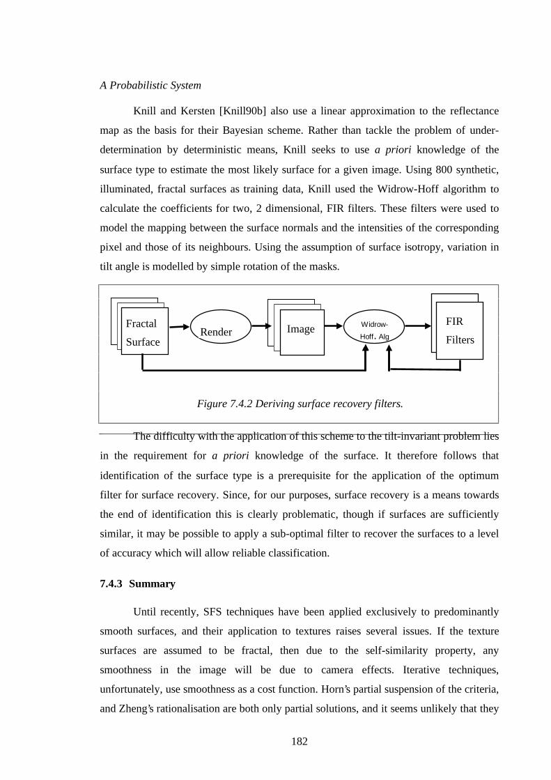
A Probabilistic System

Knill and Kersten [Knill90b] also use a linear approximation to the reflectance

map as the basis for their Bayesian scheme. Rather than tackle the problem of under-

determination by deterministic means, Knill seeks to use a priori knowledge of the

surface type to estimate the most likely surface for a given image. Using 800 synthetic,

illuminated, fractal surfaces as training data, Knill used the Widrow-Hoff algorithm to

calculate the coefficients for two, 2 dimensional, FIR filters. These filters were used to

model the mapping between the surface normals and the intensities of the corresponding

pixel and those of its neighbours. Using the assumption of surface isotropy, variation in

tilt angle is modelled by simple rotation of the masks.

The difficulty with the application of this scheme to the tilt-invariant problem lies

in the requirement for a priori knowledge of the surface. It therefore follows that

identification of the surface type is a prerequisite for the application of the optimum

filter for surface recovery. Since, for our purposes, surface recovery is a means towards

the end of identification this is clearly problematic, though if surfaces are sufficiently

similar, it may be possible to apply a sub-optimal filter to recover the surfaces to a level

of accuracy which will allow reliable classification.

7.4.3 Summary

Until recently, SFS techniques have been applied exclusively to predominantly

smooth surfaces, and their application to textures raises several issues. If the texture

surfaces are assumed to be fractal, then due to the self-similarity property, any

smoothness in the image will be due to camera effects. Iterative techniques,

unfortunately, use smoothness as a cost function. Horn’s partial suspension of the criteria,

and Zheng’s rationalisation are both only partial solutions, and it seems unlikely that they

Figure 7.4.2 Deriving surface recovery filters.

RenderWidrow-

Hoff. Alg

Fractal

SurfaceImage

FIR

Filters

183

will be effective in dealing with textures. Knill’s and Pentland's method make no

smoothness assumption and will therefore be unaffected.

Knill’s and Pentland’s techniques represent the only techniques which we have

been able to identify as being suitable for this problem. Although these schemes are both

based on linear filtering, they do, however, differ in their derivation: Pentland’s scheme

is deterministic, while Knill’s is probabilistic. Knill's technique is unsuitable for

classification by definition: in order to employ a priori knowledge, the texture type must

already be known.

In fact, closer examination of Pentland’s technique shows it to be almost identical

to the independently developed Chantler’s filters. Although developed with different

aims in mind, both techniques are derived from Kube and Pentland's linear model of the

imaging process. The differences in the techniques are due to two factors: the different

aims of the techniques and their treament of noise. In his F1 filter Chantler assumes

noise to be white, though in the F2 filter he only assumes it to be isotropic and adopts an

empirical approach to its radial frequency characteristics. Pentland assumes the noise

spectrum is proportional to the image spectrum and develops his filter accordingly. The

filters also differ in the purpose; Chantler only seeks to remove the directional effects of

illumination and implicitly recovers the magnitude of the surface derivatives. Pentland

aims to recover the surface height and therefore includes an iω term to perform the

integration of surface derivatives in the frequency domain. For our purposes these

techniques are effectively the same, and will suffer from the same difficulties. We

believe this equivalence to be quite revealing: Chantler's scheme is recovering a

physically meaningful quantity— the magnitude of the surface derivative.

7.5 A Model-Based Approach Using Photometric Stereo

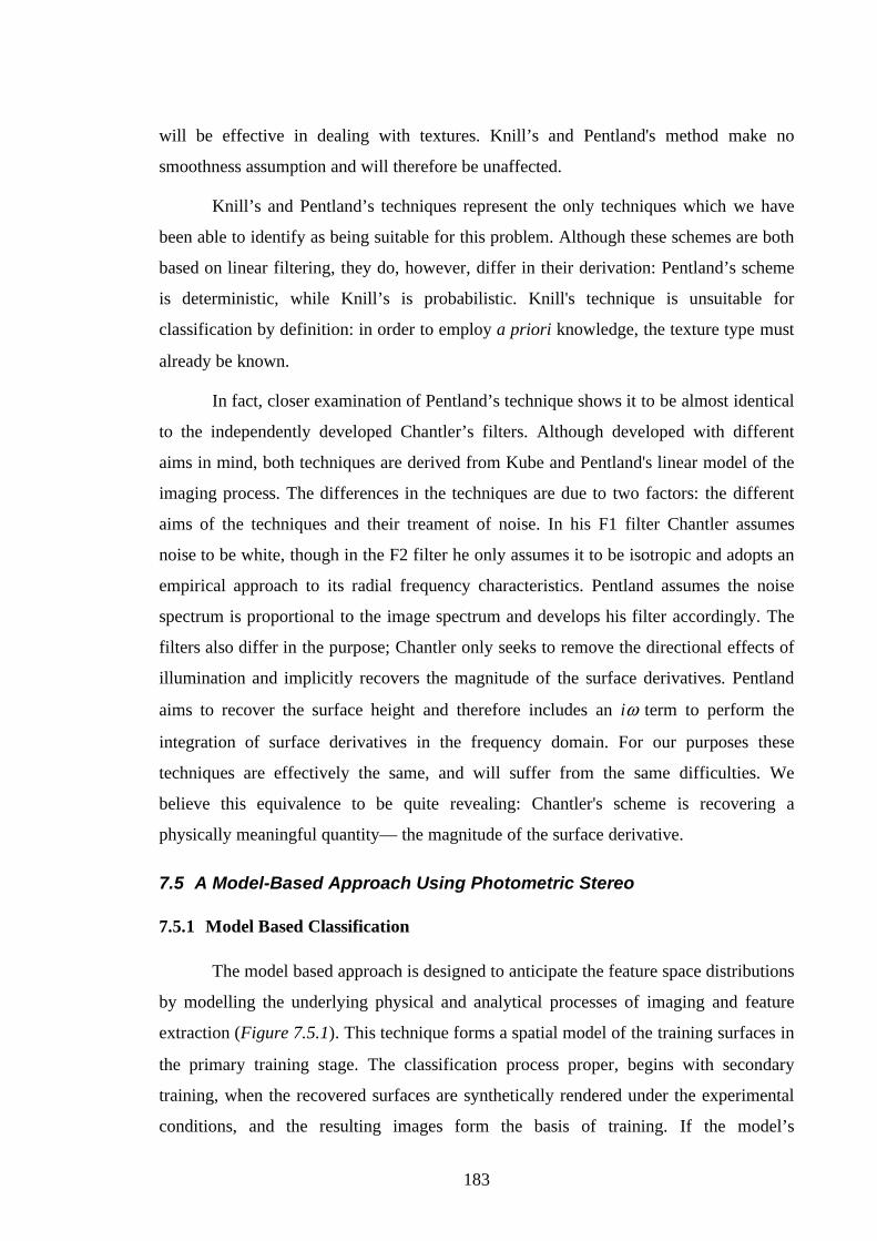
7.5.1 Model Based Classification

The model based approach is designed to anticipate the feature space distributions

by modelling the underlying physical and analytical processes of imaging and feature

extraction (Figure 7.5.1). This technique forms a spatial model of the training surfaces in

the primary training stage. The classification process proper, begins with secondary

training, when the recovered surfaces are synthetically rendered under the experimental

conditions, and the resulting images form the basis of training. If the model’s

184

components, the reflectance function and the surface description, are sufficiently

accurate we should be able to obtain classification rates approaching those of the ‘best

case’ classification, i.e. based on training on images obtained from surfaces illuminated

at that tilt angle.

SimulatedIllumination

SimulatedImage TrainingFeature

Generation

Discriminant

Image FeatureGeneration Classify

Surface

Model

Training

ImagesSFS Recovery

Training

ClassificationClassified

Image

Figure 7.5.1 Simulation Based Classification

While we have an experimentally verified reflectance model for our textures

(Chapter 3), we must still obtain the second component of the model: a description of the

surface. To do this, a method of recovery must be adopted. As we discussed earlier,

several cues to surface recovery have been investigated: focus [Noguchi94], binocular

stereo [Papadimitriou95], and laser based approaches [Gross95], have been used. Let us

assume that we will be able to invest more effort and exert more control in the recovery

stage than in the classification stages. Ideally, we seek a technique which requires no

additional hardware beyond that required for the classification.

The technique of photometric stereo allows us to form a surface description from

several images of the same surface imaged under various illumination directions. It

therefore seems ideally suited to our purposes since our problem is itself caused by

variations in illuminant direction. In fact, surface representations acquired with

photometric stereo has been used for modelling purposes by other authors. Russell

185

[Russell91] used photometric techniques to acquire depth maps which could then be

synthetically illuminated to simulate aerial images.

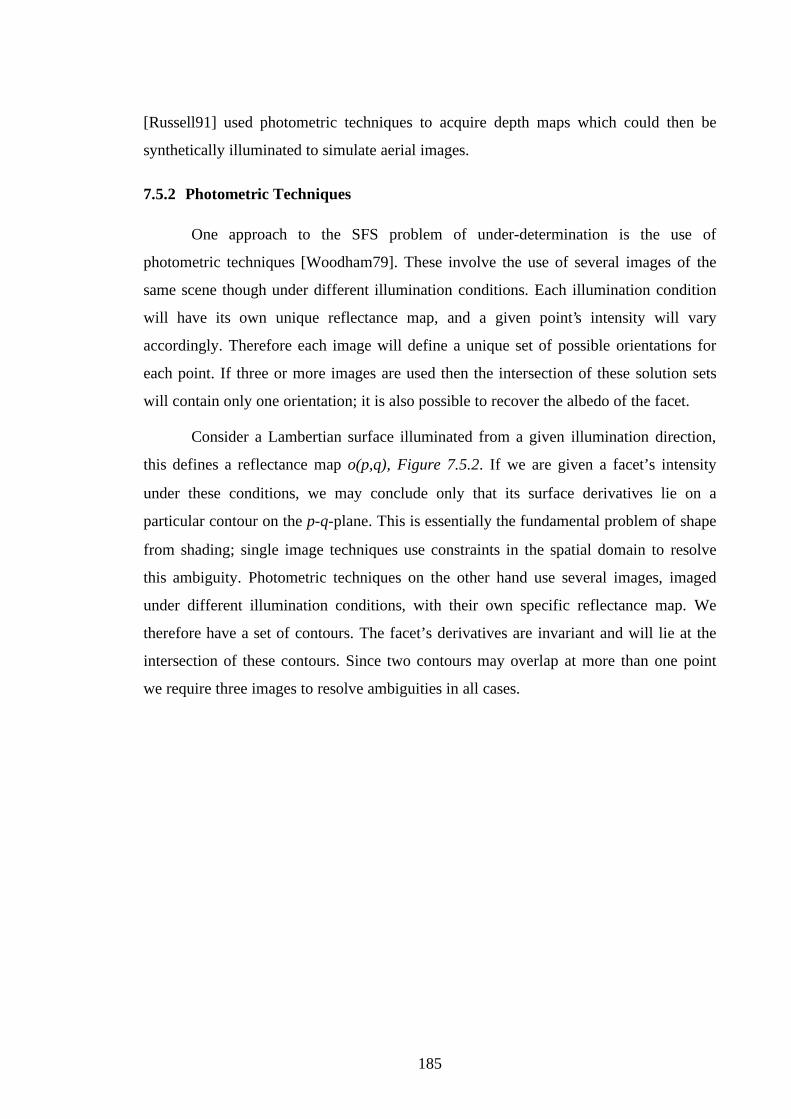
7.5.2 Photometric Techniques

One approach to the SFS problem of under-determination is the use of

photometric techniques [Woodham79]. These involve the use of several images of the

same scene though under different illumination conditions. Each illumination condition

will have its own unique reflectance map, and a given point’s intensity will vary

accordingly. Therefore each image will define a unique set of possible orientations for

each point. If three or more images are used then the intersection of these solution sets

will contain only one orientation; it is also possible to recover the albedo of the facet.

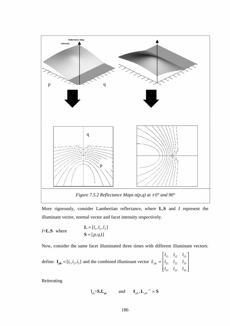
Consider a Lambertian surface illuminated from a given illumination direction,

this defines a reflectance map o(p,q), Figure 7.5.2. If we are given a facet’s intensity

under these conditions, we may conclude only that its surface derivatives lie on a

particular contour on the p-q-plane. This is essentially the fundamental problem of shape

from shading; single image techniques use constraints in the spatial domain to resolve

this ambiguity. Photometric techniques on the other hand use several images, imaged

under different illumination conditions, with their own specific reflectance map. We

therefore have a set of contours. The facet’s derivatives are invariant and will lie at the

intersection of these contours. Since two contours may overlap at more than one point

we require three images to resolve ambiguities in all cases.

186

More rigorously, consider Lambertian reflectance, where L,S and I represent the

illuminant vector, normal vector and facet intensity respectively.

I=L.S whereL

S

==

[ , , ]

[ , , ]

l l l

p q1 2 3

1

Now, consider the same facet illuminated three times with different illuminant vectors:

define: Iph = [ , , ]i i i1 2 3 and the combined illuminant vector L

l l l

l l l

l l lph =

⎡

⎣

⎢⎢⎢

⎤

⎦

⎥⎥⎥

11 12 13

21 22 23

31 32 33

Reiterating

Iph=S.Lph and I .L Sph ph− =1

Figure 7.5.2 Reflectance Maps o(p,q) at τ 0° and 90°

p q

q

p

187

While this may be solved numerically, most implementations use three dimensional

lookup tables.

In this section we have proposed a simulation based scheme which is designed to

counteract the effect of tilt on classification by predicting the location of feature space

distributions for given tilt conditions. This is achieved by using a surface and a

reflectance model to generate training data which is appropriate to classification under

the specified illumination conditions.

The surface model is an important component in the scheme. We have identified,

and given a brief description of, a technique which is capable of recovering the required

model, with relatively little overhead in terms of additional hardware and training.

7.6 Conclusions

In this chapter we considered three techniques proposed by Chantler [Chantler94]

for the reduction of tilt induced misclassification, as well as surveying the field of shape

from shading and proposing a novel simulation based technique.

Chantler’s first technique attempted to make the classifier robust by training the

classifier over the range of illumination conditions which occur during the classification

sessions. Examination of the feature means for two test textures showed that it is not safe

to employ a single threshold to discriminate between textures throughout the tilt range.

This result also showed that, in practice, the tilt angle must be known before the

classification may be undertaken.

Chantler’s second proposal advocated the use of a family of discriminants

indexed by tilt angle. Application of this technique to our test montages showed that,

while the technique is effective at reducing tilt degradation at the training angles, the

misclassification rate quickly increases as the illuminant tilt moves away from these

angles. From the performance of the classifier on our montages, we believe that a new

discriminant must be designed at intervals not exceeding 20° of tilt.

Chantler also defined a system of filters which are based on inverting the

directional effects modelled by Kube and Pentland, [Kube88]. We found application of

this scheme to be limited for two reasons. The first is the requirement that test surfaces

are isotropic; this condition is associated with the implementation of the filter estimation,

and it is possible to suggest an alternative scheme using more than one estimation image

188

to generalise the technique to directional surfaces. A more serious drawback is that of

generality; the characteristics of a filter are specific to a particular surface and any

general filter must be sub-optimal. In our experiments we found that, even with the

isotropy restriction, the sub-optimal filter is unable to stabilise the features to a

satisfactory degree. We do not pursue this approach further.

The field of single image shape from shading was reviewed. Mainstream SFS

algorithms use a smoothness constraint and are therefore unsuitable for texture

classification. Two techniques have been applied to fractal surfaces, however, implicit in

both is the requirement for a priori information as to the nature of the surface. This, by

definition, rules out these techniques from further investigation.

Finally a model based technique was proposed. This uses an estimate of the

surface derivative field obtained using photometric stereo to predict the observed texture

under specified illumination conditions. This prediction is then used to train the classifier

for those illumination conditions. The next chapter will describe the evaluation of this

technique.