Embed Size (px)
Citation preview
7.1 Introduction 139
Chapter 7
Inference for a Mean or Median
7.1 Introduction
There are many situations when we might wish to make inferences about the location
of the “center” of the population distribution of a quantitative variable. We will consider
methods for making inferences about a population mean or a population median, which are
the two most commonly used measures of the center of the distribution of a quantitative
variable, in this chapter.
In Chapter 5 we considered inferences about the distribution of a dichotomous vari-
able. Since the distribution of a dichotomous variable is completely determined by the
corresponding population success proportion, we found that the sampling distribution of
the sample proportion p was determined by the sampling method. In general, the dis-
tribution of a quantitative variable is not completely determined by a single parameter.
Therefore, before we can make inferences about the distribution of a quantitative variable
we need to make some assumptions about the distribution of the variable.
A probability model for the distribution of a discrete variableX is a theoretical relative
frequency distribution which specifies the probabilities (theoretical relative frequencies)
with which each of the possible values of X will occur. In contrast to a relative frequency
distribution, which indicates the relative frequencies with which the possible values of X
occur in a sample, a probability model or probability distribution specifies the probabilities
with which the possible values of X will occur when we observe a single value of X. That
is, if we imagine choosing a single value of X at random from all of the possible values of X,
then the probability model specifies the probability with which each possible value will be
observed. We can represent a discrete probability distribution graphically via a probability
histogram (theoretical relative frequency histogram) which is simply a histogram based on
the probabilities specified by the probability model.
A probability model for the distribution of a continuous variable X can be represented
by a density curve. A density curve is a nonnegative curve for which the area under the
curve (over the x–axis) is one. We can think of the density curve as a smooth version of
a probability histogram with the rectangles of the histogram replaced by a smooth curve
indicating where the tops of the rectangles would be. With a continuous variable X it
does not make sense to talk about the probability that X would take on a particular
value, after all if we defined positive probabilities for the infinite collection (continuum) of
possible values of X these probabilities could not add up to one. It does, however, make
sense to talk about the probability that X will take on a value in a specified interval or
range of values. Given two constants a < b the probability that X takes on a value in the
140 7.2a Introduction
interval from a to b, denoted by P (a ≤ X ≤ b), is equal to the area under the density
curve over the interval from a to b on the x–axis. Areas of this sort based on the density
curve give the probabilities which a single value of X, chosen at random from the infinite
population of possible values of X, will satisfy.
Given a probability model for the distribution of a continuous variable X, i.e., given
a density curve for the distribution of the continuous variable X, we can define population
parameters which characterize relevant aspects of the distribution. For example, we can
define the population mean µ as the balance point of the unit mass bounded by the density
curve and the number line. We can also think of the population mean as the weighted
average of the infinite collection of possible values of X with weights determined by the
density curve. We can similarly define the population median M as the point on the
number line where a vertical line would divide the area under the density curve into two
equal areas (each of size one–half).
7.2 Inference for a population mean
7.2a Introduction
In this section we will consider inference for the mean µ of the population distribution
of a continuous variable X. The basic problem we will consider is that of using a random
sample of values of the continuous variable X to estimate the corresponding population
mean or to test a hypothesis about this population mean.
Before we go further it is instructive to consider some situations where inference about
a population mean could be used and the way in which we might interpret a population
mean.
In some applications the population mean represents an actual physical constant. Let
µ denote the true value of the physical constant (such as the speed of light) which we wish
to estimate. Suppose that an experiment has been devised to produce a measurement X of
the physical constant µ. A probability model for the distribution of X provides a model for
the behavior of an observed value of X by specifying probabilities which X must satisfy.
Thus, the probability model provides an explanation of the variability in X as an estimate
of µ. It would be unreasonable to expect an observed value of X to be exactly equal to
µ; however, if the experiment is carefully planned and executed it would be reasonable to
expect the average value of X based on a long series of replications of the experiment to
be equal to µ. If this is the case, the population mean of the probability model for X will
be equal to the physical constant µ and the standard deviation σ of the probability model
will serve as a useful quantification of the variability of the measurement process.
When interest centers on an actual, physical population of units the population mean
is the average value of the variable of interest corresponding to all of the units in the

7.2a Introduction 141
population. Imagine a large population of units, e.g., a population of humans or animals.
Let the continuous variable X denote a characteristic of a unit, e.g., X might be some
measurement of the size of a unit. For concreteness, let X denote the height of an adult
human male and consider the population of all adult human males in the United Kingdom.
A probability model for the distribution of X provides a model for the behavior of an
observed value of the height X of an adult male selected at random from this population.
In this situation a probability model explains the variability among the heights of the adult
males in this population. Let µ denote the population mean height of all adult males in the
United Kingdom, i.e., let µ be the average height we would get if we averaged the heights
of all the adult males in this population. In this context the population mean height is
obviously not the “true height” of each of the adult males; however, we can think of the
height X of a particular adult male as being equal to the population mean height µ plus
or minus an adjustment for this particular male which is due to hereditary, environmental,
and other factors. The standard deviation σ of the probability model serves to quantify
the variability among this population of heights.
In many applications interest centers on the population mean difference between two
paired values. For example, consider a population of individuals with high cholesterol
levels and a drug designed to reduce cholesterol levels. Let X1 denote the cholesterol level
of an individual before taking the drug, let X2 denote this same individual’s cholesterol
level after being treated with the drug, and let D = X1−X2 denote the difference between
the two cholesterol levels (the decrease in cholesterol level). A probability model for the
distribution of D provides a model for the behavior of an observed value of the difference D
for an individual selected at random from this population. In this situation a probability
model explains the variability among the differences in cholesterol level due to treatment
with the drug for the individuals in this population. The corresponding population mean
difference µ is the average difference (decrease) in cholesterol level that we would observe if
all of the individuals in this population were treated with this drug. The standard deviation
σ of the probability model serves to quantify the variability among the differences for the
individuals in this population.
We can envision a probability model for the distribution of a quantitative variable X
in terms of a box model. If X has a finite number of possible values, then a probability
model specifies the probabilities with which these possible values will occur. If the balls
in a box are labeled with the possible values of X and the proportion of balls with each
label (value of X) in the box is equal to the probability for that value specified by the
probability model, then, according to the probability model, observing a value of X is
equivalent to selecting a single ball at random from this box and observing the label on
the ball. For a continuous variable X observing the value of X is like selecting a ball at
random from a box containing an infinite collection of suitably labeled balls.
142 7.2a Introduction
Given a probability model for the distribution of X, a collection of n values of X is
said to form a random sample of size n if it satisfies the two properties given below.
1. Each value of the variable X that we observe can be viewed as a single value
chosen at random from a (usually infinite) population of values which are distributed
according to the specified probability model for the distribution of X.
2. The observed values of X are independent. That is, knowing the value of one or
more of the observed values of X has no effect on the probabilities associated with
other values of X.
In other words, in terms of the box model for the probability distribution of X a random
sample of n values of X can be viewed as a collection of n labels corresponding to a simple
random sample selected with replacement from a box of suitably labeled balls.
Given a random sample of values of X it seems obvious that the sample mean X is an
appropriate estimate of the corresponding population mean µ. The sampling distribution
of X, which describes the sample to sample variability in X, serves as the starting point
for our study of the behavior of the sample mean X as an estimator of the population
mean µ. The exact form of the sampling distribution of X depends on the form of the
distribution of X. However, the two important properties of the sampling distribution of
the sample mean given below are valid regardless of the exact form of the distribution of
X.
Let X denote the sample mean of a random sample of size n from a population
(distribution) with population mean µ and population standard deviation σ. The sampling
distribution of the sample mean X has the following characteristics.
1. The mean of the sampling distribution of X is the corresponding population mean
µ. This indicates that the sample meanX is unbiased as an estimator of the population
mean µ. Recall that saying that a statistic is unbiased means that, even though the
statistic will overestimate the parameter for some samples and will underestimate the
parameter in other samples, it will do so in such a way that, in the long run, the
values of the statistic will average to give the correct value of the parameter.
2. The population standard error of the sample mean X (the standard deviation of
the sampling distribution of X) is S.E.(X) = σ/√n. That is, the standard deviation
of the sampling distribution of X is equal to the standard deviation of the distribution
of X divided by the square root of the sample size. Notice that this implies that the
sample mean is less variable than a single observation as an estimator of µ; and that
if µ and σ are held constant, then the variability in X as an estimator of µ decreases
as the sample size increases reflecting the fact that a larger sample provides more
information than a smaller sample.

7.2b The normal distribution 143
Since the form of the sampling distribution of X depends on the form of the distribu-
tion of X, we will need to make some assumptions about the distribution of X before we
can proceed with our discussion of inference for the population mean µ. These assumptions
correspond to the choice of a probability model (density curve) to represent the distribu-
tion of X. There is an infinite collection of probability models to choose from but we will
restrict our attention to a single probability model, the normal probability model, which
is appropriate for many situations when the distribution of X is symmetric and mound
shaped. This does not imply that all, or even most, distributions of continuous variables
are normal distributions. Some of the reasons that we will use the normal distribution as
a probability model are: (1) the theory needed for inference has been worked out for the
normal model; (2) there are many situations where a normal distribution provides a rea-
sonable model for the distribution of a quantitative variable; (3) even though the inferential
methods we discuss are based on the assumption that the distribution of the variable is
exactly a normal distribution, it is known that these inferential methods actually perform
reasonably well provided the true distribution of the variable is “reasonably similar to a
normal distribution”; and, (4) it is often possible to transform or redefine a variable so
that its distribution is reasonably modeled by a normal distribution.
7.2b The normal distribution
The normal distribution with mean µ and standard deviation σ can be characterized by
its density curve. The density curve for the normal distribution with mean µ and standard
deviation σ is the familiar bell shaped curve. The standard normal density curve, which
has mean µ = 0 and standard deviation σ = 1, is shown in Figure 1.
Figure 1. The standard normal density curve.
-4 -2 0 2 4
Z
The normal distribution with mean µ and its density curve are symmetric around µ, i.e.,
if we draw a vertical line through µ, then the two sides of the density curve are mirror
images of each other. Therefore the mean of a normal distribution µ is also the median of
the normal distribution. The mean µ locates the normal distribution on the number line so

144 7.2b The normal distribution
that if we hold σ constant and change the mean µ, the normal distribution is simply shifted
along the number line until it is centered at the new mean. In other words, holding σ fixed
and changing µ simply relocates the density curve on the number line; it has no effect on
the shape of the curve. Figure 2 provides the density curves for normal distributions with
respective means µ = 0 and µ = 2 and common standard deviation σ = 1.
Figure 2. Normal distributions with common standard deviation one andmeans of zero and two.
-2 0 2 4X
mean 0mean 2
The standard deviation σ indicates the amount of variability in the normal distribu-
tion. If we hold µ fixed and increase the value of σ, then the normal density curve becomes
flatter, while retaining its bell–shape, indicating that there is more variability in the distri-
bution. Similarly, if we hold µ fixed and decrease the value of σ, then the normal density
curve becomes more peaked around the mean µ, while retaining its bell–shape, indicating
that there is less variability in the distribution. Normal distributions with mean µ = 0
and respective standard deviations σ = .5, σ = 1, and σ = 2 are plotted in Figure 3.
Figure 3. Normal distributions with common mean zero and standarddeviations one–half, one, and two.
-5 -3 -1 1 3 5
X
std. dev. 1/2std. dev. 1std. dev. 2
Example. Heights of adult males. The 8585 heights (in inches) of adult males
born in the United Kingdom (including the whole of Ireland) which are summarized in

7.2b The normal distribution 145
Table 8 of Section 3.3 provide a good illustration of the fact that normal distributions
often provide very good models for populations of physical measurements, such as heights
or weights, of individuals. Figure 4 provides a histogram for this height distribution and
the density curve for a normal distribution chosen to model these data. You can see that
the normal distribution provides a very reasonable model for the heights of adult males
born in the United Kingdom.
Figure 4. Histogram and normal density curve for the UK height example.
57 59 61 63 65 67 69 71 73 75 77height
Computer programs and many calculators can be used to compute normal probabilities
or equivalently to compute areas under the normal density curve. These probabilities can
also be calculated using tables of standard normal distribution probabilities such as Table
1. Recall that the standard normal distribution is the normal distribution with mean µ = 0
and standard deviation σ = 1. The relationship between the standard normal variable Z
and the normal variable X, which has mean µ and standard deviation σ, is
Z =X − µ
σor equivalently X = µ+ Zσ.
This relationship implies that a probability statement about the normal variable X can
be re–expressed as a probability statement about the standard normal variable Z by re–
expressing the statement in terms of standard deviation units from the mean. Given
two constants a < b, observing a value of X between a and b (observing a ≤ X ≤ b)
is equivalent to observing a value of Z = (X − µ)/σ between (a − µ)/σ and (b − µ)/σ
(observing (a − µ)/σ ≤ (X − µ)/σ ≤ (b − µ)/σ). Furthermore, Z = (X − µ)/σ behaves
in accordance with the standard normal distribution so that the probability of observing
a value of X between a and b, denoted by P (a ≤ X ≤ b), is equal to the probability that
the standard normal variable Z takes on a value between (a− µ)/σ and (b− µ)/σ, i.e.,
146 7.2b The normal distribution
P (a ≤ X ≤ b) = P
(a− µ
σ≤ Z ≤ b− µ
σ
).
In terms of areas this probability equality says that the area under the normal density
curve with mean µ and standard deviation σ over the interval from a to b is equal to the
area under the standard normal density curve over the interval from (a−µ)/σ to (b−µ)/σ.Similarly, given constants c < d, we have the analogous result that
P (c ≤ Z ≤ d) = P (µ+ cσ ≤ X ≤ µ+ dσ).
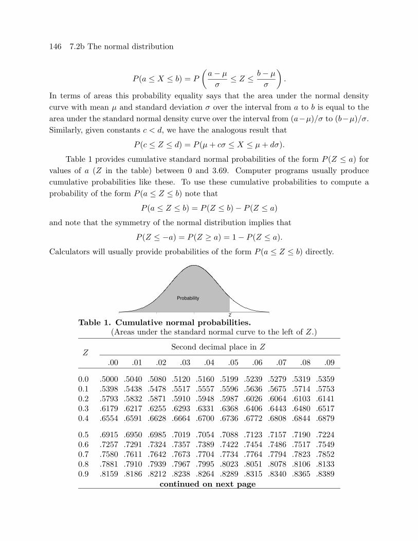
Table 1 provides cumulative standard normal probabilities of the form P (Z ≤ a) for
values of a (Z in the table) between 0 and 3.69. Computer programs usually produce
cumulative probabilities like these. To use these cumulative probabilities to compute a
probability of the form P (a ≤ Z ≤ b) note that
P (a ≤ Z ≤ b) = P (Z ≤ b)− P (Z ≤ a)
and note that the symmetry of the normal distribution implies that
P (Z ≤ −a) = P (Z ≥ a) = 1− P (Z ≤ a).
Calculators will usually provide probabilities of the form P (a ≤ Z ≤ b) directly.
Z
Probability
Table 1. Cumulative normal probabilities.(Areas under the standard normal curve to the left of Z.)
Second decimal place in ZZ
.00 .01 .02 .03 .04 .05 .06 .07 .08 .09
0.0 .5000 .5040 .5080 .5120 .5160 .5199 .5239 .5279 .5319 .53590.1 .5398 .5438 .5478 .5517 .5557 .5596 .5636 .5675 .5714 .57530.2 .5793 .5832 .5871 .5910 .5948 .5987 .6026 .6064 .6103 .61410.3 .6179 .6217 .6255 .6293 .6331 .6368 .6406 .6443 .6480 .65170.4 .6554 .6591 .6628 .6664 .6700 .6736 .6772 .6808 .6844 .6879
0.5 .6915 .6950 .6985 .7019 .7054 .7088 .7123 .7157 .7190 .72240.6 .7257 .7291 .7324 .7357 .7389 .7422 .7454 .7486 .7517 .75490.7 .7580 .7611 .7642 .7673 .7704 .7734 .7764 .7794 .7823 .78520.8 .7881 .7910 .7939 .7967 .7995 .8023 .8051 .8078 .8106 .81330.9 .8159 .8186 .8212 .8238 .8264 .8289 .8315 .8340 .8365 .8389
continued on next page
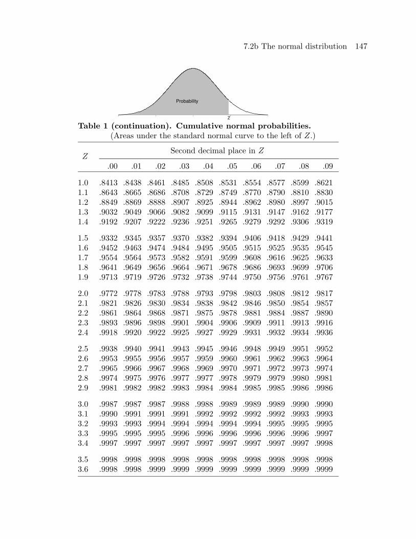
7.2b The normal distribution 147
Z
Probability
Table 1 (continuation). Cumulative normal probabilities.(Areas under the standard normal curve to the left of Z.)
Second decimal place in ZZ
.00 .01 .02 .03 .04 .05 .06 .07 .08 .09
1.0 .8413 .8438 .8461 .8485 .8508 .8531 .8554 .8577 .8599 .86211.1 .8643 .8665 .8686 .8708 .8729 .8749 .8770 .8790 .8810 .88301.2 .8849 .8869 .8888 .8907 .8925 .8944 .8962 .8980 .8997 .90151.3 .9032 .9049 .9066 .9082 .9099 .9115 .9131 .9147 .9162 .91771.4 .9192 .9207 .9222 .9236 .9251 .9265 .9279 .9292 .9306 .9319
1.5 .9332 .9345 .9357 .9370 .9382 .9394 .9406 .9418 .9429 .94411.6 .9452 .9463 .9474 .9484 .9495 .9505 .9515 .9525 .9535 .95451.7 .9554 .9564 .9573 .9582 .9591 .9599 .9608 .9616 .9625 .96331.8 .9641 .9649 .9656 .9664 .9671 .9678 .9686 .9693 .9699 .97061.9 .9713 .9719 .9726 .9732 .9738 .9744 .9750 .9756 .9761 .9767
2.0 .9772 .9778 .9783 .9788 .9793 .9798 .9803 .9808 .9812 .98172.1 .9821 .9826 .9830 .9834 .9838 .9842 .9846 .9850 .9854 .98572.2 .9861 .9864 .9868 .9871 .9875 .9878 .9881 .9884 .9887 .98902.3 .9893 .9896 .9898 .9901 .9904 .9906 .9909 .9911 .9913 .99162.4 .9918 .9920 .9922 .9925 .9927 .9929 .9931 .9932 .9934 .9936
2.5 .9938 .9940 .9941 .9943 .9945 .9946 .9948 .9949 .9951 .99522.6 .9953 .9955 .9956 .9957 .9959 .9960 .9961 .9962 .9963 .99642.7 .9965 .9966 .9967 .9968 .9969 .9970 .9971 .9972 .9973 .99742.8 .9974 .9975 .9976 .9977 .9977 .9978 .9979 .9979 .9980 .99812.9 .9981 .9982 .9982 .9983 .9984 .9984 .9985 .9985 .9986 .9986
3.0 .9987 .9987 .9987 .9988 .9988 .9989 .9989 .9989 .9990 .99903.1 .9990 .9991 .9991 .9991 .9992 .9992 .9992 .9992 .9993 .99933.2 .9993 .9993 .9994 .9994 .9994 .9994 .9994 .9995 .9995 .99953.3 .9995 .9995 .9995 .9996 .9996 .9996 .9996 .9996 .9996 .99973.4 .9997 .9997 .9997 .9997 .9997 .9997 .9997 .9997 .9997 .9998
3.5 .9998 .9998 .9998 .9998 .9998 .9998 .9998 .9998 .9998 .99983.6 .9998 .9998 .9999 .9999 .9999 .9999 .9999 .9999 .9999 .9999
148 7.2c Sampling from a normal population
7.2c Sampling from a normal population
Strictly speaking, the inferential methods based on the Student’s t distribution de-
scribed in Sections 7.2d and 7.2e are only appropriate when the data constitute a random
sample from a normal population. However, these methods are known to be generally
reasonable even when the underlying population is not exactly a normal population, pro-
vided the underlying population distribution is reasonably symmetric and the true density
curve has a more or less normal (bell–shaped) appearance. We cannot be sure that an
underlying population is normal; however, we can use descriptive methods to look for ev-
idence of possible nonnormality, provided the sample size is reasonably large. The most
easily detected and serious evidence of nonnormality you should look for is evidence of
extreme skewness or evidence of extreme outlying observations. If there is evidence of
extreme skewness or extreme outlying observations, then the inferential methods based on
the Student’s t distribution should not be used. An alternate approach to inference (for a
population median) which may be used when the Student’s t methods are inappropriate
is discussed in Section 7.3.
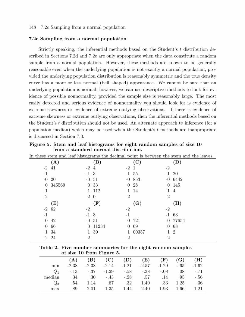
Figure 5. Stem and leaf histograms for eight random samples of size 10from a standard normal distribution.
In these stem and leaf histograms the decimal point is between the stem and the leaves.
(A) (B) (C) (D)-2 41 -2 4 -2 1 -2-1 -1 3 -1 55 -1 20-0 20 -0 51 -0 853 -0 64420 345569 0 33 0 28 0 1451 1 112 1 14 1 42 2 0 2 2
(E) (F) (G) (H)-2 62 -2 -2 -2-1 -1 3 -1 -1 63-0 42 -0 51 -0 721 -0 776540 66 0 11234 0 69 0 681 34 1 39 1 00357 1 22 24 2 2 2
Table 2. Five number summaries for the eight random samplesof size 10 from Figure 5.
(A) (B) (C) (D) (E) (F) (G) (H)min -2.38 -2.38 -2.14 -1.21 -2.57 -1.29 -.65 -1.62Q1 -.13 -.37 -1.29 -.58 -.38 -.08 .08 -.71
median .34 .30 -.43 -.28 .57 .14 .95 -.56Q3 .54 1.14 .67 .32 1.40 .33 1.25 .36max .89 2.01 1.35 1.44 2.40 1.93 1.66 1.21
7.2c Sampling from a normal population 149
Using a sample to determine whether the underlying population is normal requires
some practice. Some indication of the sorts of samples which may arise when the under-
lying population is normal is provided by the stem and leaf histograms and five number
summaries given in Figures 5 and 6 and Tables 2 and 3 for several computer generated
random samples from a standard normal distribution. The eight random samples of size
10 of Figure 5 and Table 2 indicate what may happen when a small sample is taken from
a population which is normal. Based on these examples it is clear that we should not
necessarily view slight skewness (as in A, B, D, F, G, and H) or mild outliers (as in A
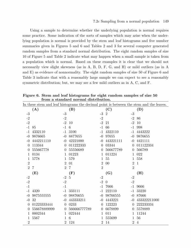
and E) as evidence of nonnormality. The eight random samples of size 50 of Figure 6 and
Table 3 indicate that with a reasonably large sample we can expect to see a reasonably
symmetric distribution; but, we may see a few mild outliers as in A, C, and F.
Figure 6. Stem and leaf histograms for eight random samples of size 50from a standard normal distribution.
In these stem and leaf histograms the decimal point is between the stem and the leaves.
(A) (B) (C) (D)-3 -3 -3 2 -3-2 -2 -2 -2 86-2 -2 10 -2 21 -2 10-1 85 -1 6 -1 66 -1 998-1 4332110 -1 3100 -1 4322110 -1 4443222-0 9876665 -0 8877655 -0 97655 -0 9876655-0 4442211110 -0 42221000 -0 443221111 -0 44211110 113344 0 011222333 0 03344 0 0111223340 555667778 0 55556689 0 566677789 0 5667891 0134 1 01223 1 011224 1 0221 5778 1 579 1 55 1 5582 2 01 2 00 2 12 7 2 7 2 2
(E) (F) (G) (H)-2 -2 5 -2 -2-2 -2 -2 0 -2-1 -1 -1 7666 -1 9666-1 4320 -1 333111 -1 222110 -1 33220-0 9875555555 -0 98876655 -0 98766555 -0 87666-0 32 -0 443333211 -0 4443221 -0 4333222110000 01223333444 0 0233 0 122223 0 2222333340 556678889999 0 566666777789 0 6678899 0 55788891 0002344 1 022444 1 011 1 112441 5567 1 6 1 555699 1 562 2 124 2 14 2 4
150 7.2c Sampling from a normal population
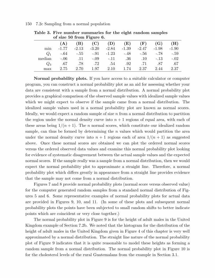
Table 3. Five number summaries for the eight random samplesof size 50 from Figure 6.
(A) (B) (C) (D) (E) (F) (G) (H)min -1.77 -2.13 -3.20 -2.84 -1.39 -2.47 -1.98 -1.90Q1 -.64 -.55 -.91 -1.23 -.48 -.56 -.78 -.59
median -.06 .11 -.09 -.11 .36 .10 -.13 -.02Q3 .67 .78 .72 .54 .92 .71 .87 .67max 2.75 2.70 1.97 2.10 1.74 2.37 2.44 2.37
Normal probability plots. If you have access to a suitable calculator or computer
program, you can construct a normal probability plot as an aid for assessing whether your
data are consistent with a sample from a normal distribution. A normal probability plot
provides a graphical comparison of the observed sample values with idealized sample values
which we might expect to observe if the sample came from a normal distribution. The
idealized sample values used in a normal probability plot are known as normal scores.
Ideally, we would expect a random sample of size n from a normal distribution to partition
the region under the normal density curve into n + 1 regions of equal area, with each of
these areas being 1/(n+ 1). The n normal scores, which constitute our idealized random
sample, can thus be formed by determining the n values which would partition the area
under the normal density curve into n + 1 regions each of area 1/(n + 1) as suggested
above. Once these normal scores are obtained we can plot the ordered normal scores
versus the ordered observed data values and examine this normal probability plot looking
for evidence of systematic disagreement between the actual sample values and the expected
normal scores. If the sample really was a sample from a normal distribution, then we would
expect the normal probability plot to approximate a straight line. Therefore, a normal
probability plot which differs greatly in appearance from a straight line provides evidence
that the sample may not come from a normal distribution.
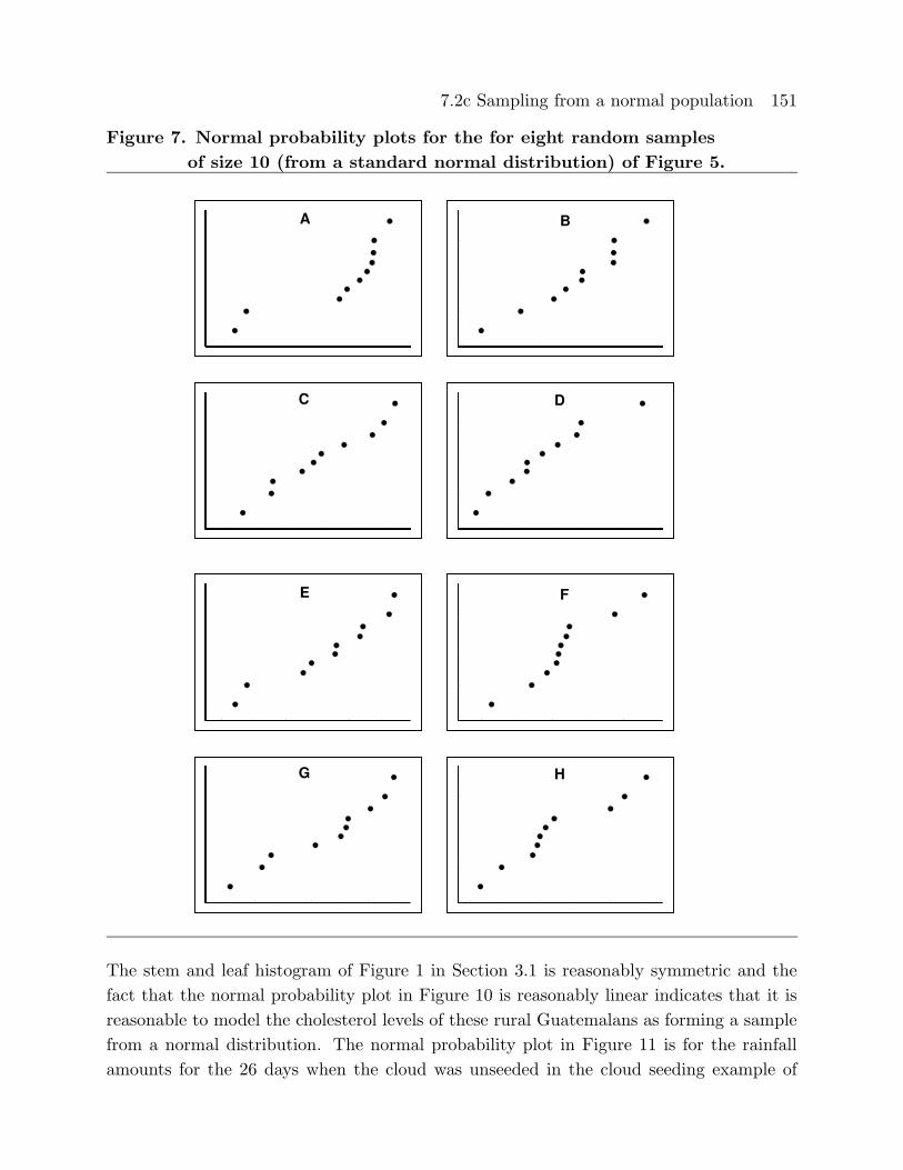
Figures 7 and 8 provide normal probability plots (normal score versus observed value)
for the computer generated random samples from a standard normal distribution of Fig-
ures 5 and 6. Some representative examples of normal probability plots for actual data
are provided in Figures 9, 10, and 11. (In some of these plots and subsequent normal
probability plots the points have been subjected to small random shifts to better indicate
points which are coincident or very close together.)
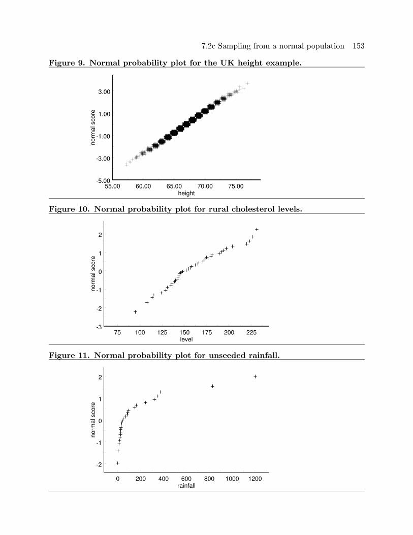
The normal probability plot in Figure 9 is for the height of adult males in the United
Kingdom example of Section 7.2b. We noted that the histogram for the distribution of the
height of adult males in the United Kingdom given in Figure 4 of this chapter is very well
approximated by a normal distribution. The straight line nature of the normal probability
plot of Figure 9 indicates that it is quite reasonable to model these heights as forming a
random sample from a normal distribution. The normal probability plot in Figure 10 is
for the cholesterol levels of the rural Guatemalans from the example in Section 3.1.
7.2c Sampling from a normal population 151
Figure 7. Normal probability plots for the for eight random samples
of size 10 (from a standard normal distribution) of Figure 5.
A B
DC
E F
HG
The stem and leaf histogram of Figure 1 in Section 3.1 is reasonably symmetric and the
fact that the normal probability plot in Figure 10 is reasonably linear indicates that it is
reasonable to model the cholesterol levels of these rural Guatemalans as forming a sample
from a normal distribution. The normal probability plot in Figure 11 is for the rainfall
amounts for the 26 days when the cloud was unseeded in the cloud seeding example of
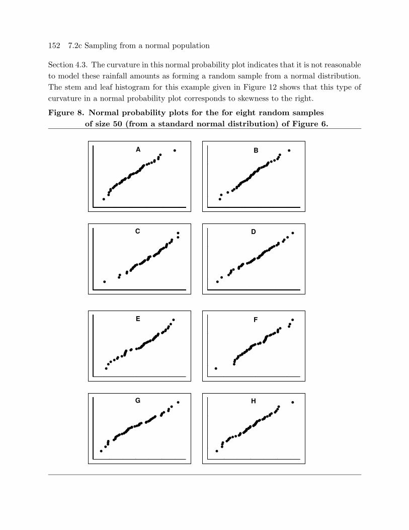
152 7.2c Sampling from a normal population
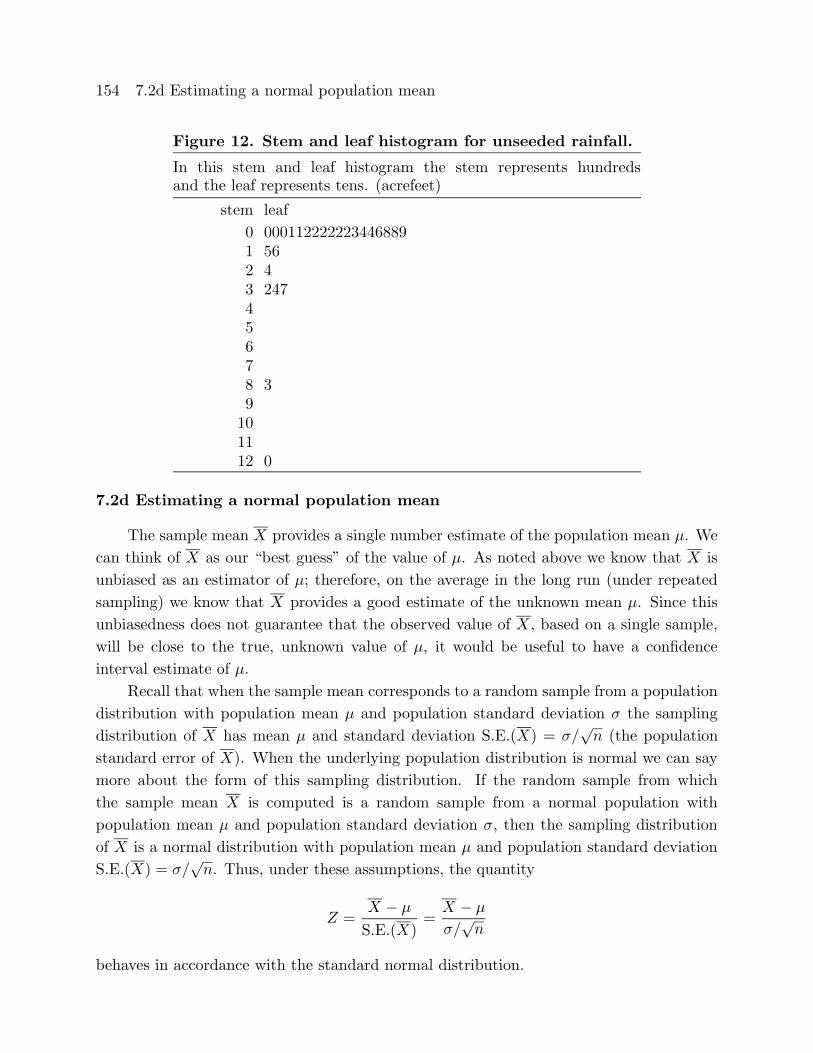
Section 4.3. The curvature in this normal probability plot indicates that it is not reasonable
to model these rainfall amounts as forming a random sample from a normal distribution.
The stem and leaf histogram for this example given in Figure 12 shows that this type of
curvature in a normal probability plot corresponds to skewness to the right.
Figure 8. Normal probability plots for the for eight random samples
of size 50 (from a standard normal distribution) of Figure 6.
A B
DC
E F
HG
7.2c Sampling from a normal population 153
Figure 9. Normal probability plot for the UK height example.
55.00 60.00 65.00 70.00 75.00height
-5.00
-3.00
-1.00
1.00
3.00no
rmal
sco
re
Figure 10. Normal probability plot for rural cholesterol levels.
75 100 125 150 175 200 225level
-3
-2
-1
0
1
2
norm
al s
core
Figure 11. Normal probability plot for unseeded rainfall.
0 200 400 600 800 1000 1200rainfall
-2
-1
0
1
2
norm
al s
core
154 7.2d Estimating a normal population mean
Figure 12. Stem and leaf histogram for unseeded rainfall.
In this stem and leaf histogram the stem represents hundredsand the leaf represents tens. (acrefeet)
stem leaf
0 0001122222234468891 562 43 24745678 39101112 0
7.2d Estimating a normal population mean
The sample mean X provides a single number estimate of the population mean µ. We
can think of X as our “best guess” of the value of µ. As noted above we know that X is
unbiased as an estimator of µ; therefore, on the average in the long run (under repeated
sampling) we know that X provides a good estimate of the unknown mean µ. Since this
unbiasedness does not guarantee that the observed value of X, based on a single sample,
will be close to the true, unknown value of µ, it would be useful to have a confidence
interval estimate of µ.
Recall that when the sample mean corresponds to a random sample from a population
distribution with population mean µ and population standard deviation σ the sampling
distribution of X has mean µ and standard deviation S.E.(X) = σ/√n (the population
standard error of X). When the underlying population distribution is normal we can say
more about the form of this sampling distribution. If the random sample from which
the sample mean X is computed is a random sample from a normal population with
population mean µ and population standard deviation σ, then the sampling distribution
of X is a normal distribution with population mean µ and population standard deviation
S.E.(X) = σ/√n. Thus, under these assumptions, the quantity
Z =X − µ
S.E.(X)=
X − µ
σ/√n
behaves in accordance with the standard normal distribution.

7.2d Estimating a normal population mean 155
We know that a standard normal variable Z will take on a value between −1.96 and1.96 with probability .95 (P (−1.96 ≤ Z ≤ 1.96) = .95). This implies that
P
(−1.96 ≤ X − µ
S.E.(X)≤ 1.96
)= .95
which is equivalent to
P(X − 1.96S.E.(X) ≤ µ ≤ X + 1.96S.E.(X)
)= .95.
This probability statement says that 95% of the time we will observe a value of X such
that the population mean µ will be between X − 1.96S.E.(X) and X + 1.96S.E.(X). Un-fortunately, we cannot use this interval as a confidence interval for µ, since the population
standard error S.E.(X) = σ/√n depends on the unknown population standard deviation
σ and thus is not computable. We can avoid this difficulty by replacing the unknown
population standard error σ/√n by the sample standard error S.E.(X) = S/
√n, where
S is the sample standard deviation, and basing our confidence interval estimate on the
quantity
T =X − µ
S.E.(X)=
X − µ
S/√n.
If the sample mean X and the sample standard deviation S are computed from a
random sample of size n from a normal population with population mean µ and popu-
lation standard deviation σ, then the quantity T defined above follows the Student’s t
distribution with n− 1 degrees of freedom. The Student’s t distribution with n− 1degrees of freedom is symmetric about zero and has a density curve very similar to that of
the standard normal distribution. The main difference between these two distributions is
that the Student’s t distribution has “heavier” tails than the standard normal distribution.
That is, the tails of the Student’s t density curve approach the x–axis more slowly than
do the tails of the standard normal density curve. As the sample size (and the degrees
of freedom) increases the Student’s t distribution becomes more similar to the standard
normal distribution. In fact, the standard normal distribution is the limiting version of
the Student’s t distribution in the sense that the Student’s t density curve approaches
the standard normal density curve when the degrees of freedom increases without bound.
The relationship between Student’s t distributions and the standard normal distribution
is indicated by the plots in Figure 13.
156 7.2d Estimating a normal population mean
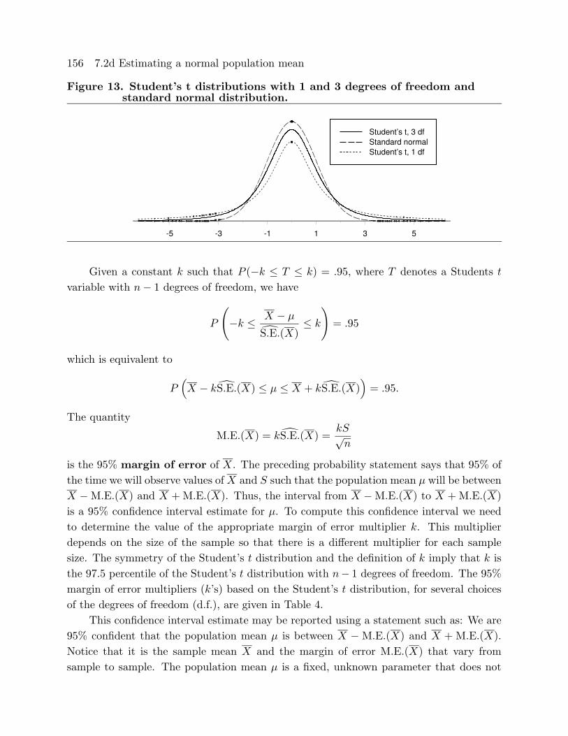
Figure 13. Student’s t distributions with 1 and 3 degrees of freedom andstandard normal distribution.
-5 -3 -1 1 3 5
Student’s t, 3 dfStandard normalStudent’s t, 1 df
Given a constant k such that P (−k ≤ T ≤ k) = .95, where T denotes a Students t
variable with n− 1 degrees of freedom, we have
P
(−k ≤ X − µ
S.E.(X)≤ k
)= .95
which is equivalent to
P(X − kS.E.(X) ≤ µ ≤ X + kS.E.(X)
)= .95.
The quantity
M.E.(X) = kS.E.(X) =kS√n
is the 95% margin of error of X. The preceding probability statement says that 95% of
the time we will observe values ofX and S such that the population mean µ will be between
X −M.E.(X) and X +M.E.(X). Thus, the interval from X −M.E.(X) to X +M.E.(X)is a 95% confidence interval estimate for µ. To compute this confidence interval we need
to determine the value of the appropriate margin of error multiplier k. This multiplier
depends on the size of the sample so that there is a different multiplier for each sample
size. The symmetry of the Student’s t distribution and the definition of k imply that k is
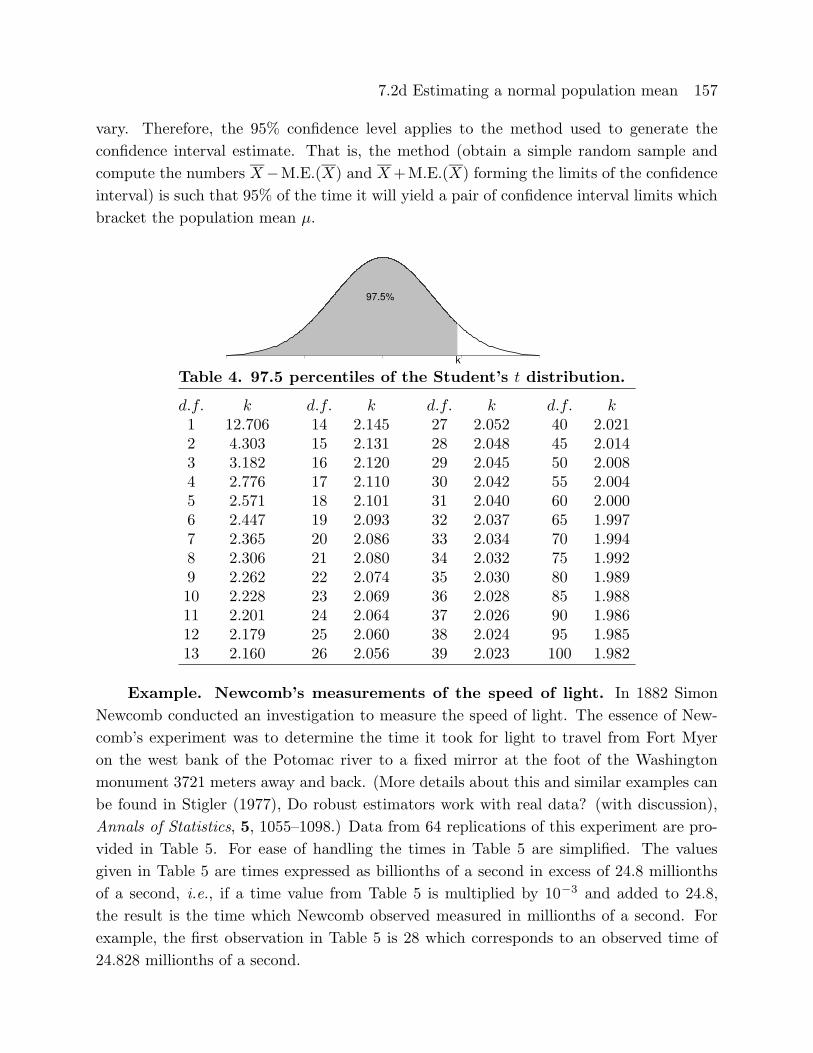
the 97.5 percentile of the Student’s t distribution with n− 1 degrees of freedom. The 95%margin of error multipliers (k’s) based on the Student’s t distribution, for several choices
of the degrees of freedom (d.f.), are given in Table 4.
This confidence interval estimate may be reported using a statement such as: We are
95% confident that the population mean µ is between X −M.E.(X) and X + M.E.(X).
Notice that it is the sample mean X and the margin of error M.E.(X) that vary from
sample to sample. The population mean µ is a fixed, unknown parameter that does not
7.2d Estimating a normal population mean 157
vary. Therefore, the 95% confidence level applies to the method used to generate the
confidence interval estimate. That is, the method (obtain a simple random sample and
compute the numbers X−M.E.(X) and X+M.E.(X) forming the limits of the confidenceinterval) is such that 95% of the time it will yield a pair of confidence interval limits which
bracket the population mean µ.
97.5%
k
Table 4. 97.5 percentiles of the Student’s t distribution.
d.f. k d.f. k d.f. k d.f. k1 12.706 14 2.145 27 2.052 40 2.0212 4.303 15 2.131 28 2.048 45 2.0143 3.182 16 2.120 29 2.045 50 2.0084 2.776 17 2.110 30 2.042 55 2.0045 2.571 18 2.101 31 2.040 60 2.0006 2.447 19 2.093 32 2.037 65 1.9977 2.365 20 2.086 33 2.034 70 1.9948 2.306 21 2.080 34 2.032 75 1.9929 2.262 22 2.074 35 2.030 80 1.98910 2.228 23 2.069 36 2.028 85 1.98811 2.201 24 2.064 37 2.026 90 1.98612 2.179 25 2.060 38 2.024 95 1.98513 2.160 26 2.056 39 2.023 100 1.982
Example. Newcomb’s measurements of the speed of light. In 1882 Simon
Newcomb conducted an investigation to measure the speed of light. The essence of New-
comb’s experiment was to determine the time it took for light to travel from Fort Myer
on the west bank of the Potomac river to a fixed mirror at the foot of the Washington
monument 3721 meters away and back. (More details about this and similar examples can
be found in Stigler (1977), Do robust estimators work with real data? (with discussion),
Annals of Statistics, 5, 1055–1098.) Data from 64 replications of this experiment are pro-
vided in Table 5. For ease of handling the times in Table 5 are simplified. The values
given in Table 5 are times expressed as billionths of a second in excess of 24.8 millionths
of a second, i.e., if a time value from Table 5 is multiplied by 10−3 and added to 24.8,
the result is the time which Newcomb observed measured in millionths of a second. For
example, the first observation in Table 5 is 28 which corresponds to an observed time of
24.828 millionths of a second.

158 7.2d Estimating a normal population mean
Table 5. Newcomb’s time data.
28 22 36 26 28 28 26 24 32 30 27 24 33 21 36 3231 25 24 25 28 36 27 32 34 30 25 26 26 25 23 2130 33 29 27 29 28 22 26 27 16 31 29 36 32 28 4019 37 23 32 29 24 25 27 24 16 29 20 28 27 39 23
Figure 14. Stem and leaf histogram for Newcomb’s time data.
In this stem and leaf histogram the stem represents tens of billionths ofa second and the leaf represents billionths of a second.
stem leaf1 661 92 0112 223332 44444555552 666667777772 8888888999993 000113 22222333 43 666673 94 0
Figure 15. Normal probability plot for Newcomb’s time data.
15 20 25 30 35 40time
-3
-2
-1
0
1
2
norm
al s
core
7.2d Estimating a normal population mean 159
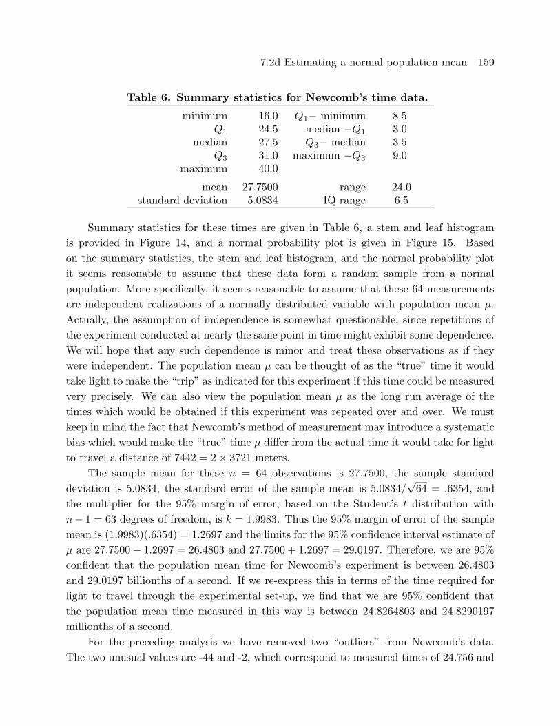
Table 6. Summary statistics for Newcomb’s time data.
minimum 16.0 Q1− minimum 8.5Q1 24.5 median −Q1 3.0
median 27.5 Q3− median 3.5Q3 31.0 maximum −Q3 9.0
maximum 40.0
mean 27.7500 range 24.0standard deviation 5.0834 IQ range 6.5
Summary statistics for these times are given in Table 6, a stem and leaf histogram
is provided in Figure 14, and a normal probability plot is given in Figure 15. Based
on the summary statistics, the stem and leaf histogram, and the normal probability plot
it seems reasonable to assume that these data form a random sample from a normal
population. More specifically, it seems reasonable to assume that these 64 measurements
are independent realizations of a normally distributed variable with population mean µ.
Actually, the assumption of independence is somewhat questionable, since repetitions of
the experiment conducted at nearly the same point in time might exhibit some dependence.
We will hope that any such dependence is minor and treat these observations as if they
were independent. The population mean µ can be thought of as the “true” time it would
take light to make the “trip” as indicated for this experiment if this time could be measured
very precisely. We can also view the population mean µ as the long run average of the
times which would be obtained if this experiment was repeated over and over. We must
keep in mind the fact that Newcomb’s method of measurement may introduce a systematic
bias which would make the “true” time µ differ from the actual time it would take for light
to travel a distance of 7442 = 2× 3721 meters.The sample mean for these n = 64 observations is 27.7500, the sample standard
deviation is 5.0834, the standard error of the sample mean is 5.0834/√64 = .6354, and
the multiplier for the 95% margin of error, based on the Student’s t distribution with
n− 1 = 63 degrees of freedom, is k = 1.9983. Thus the 95% margin of error of the samplemean is (1.9983)(.6354) = 1.2697 and the limits for the 95% confidence interval estimate of
µ are 27.7500− 1.2697 = 26.4803 and 27.7500 + 1.2697 = 29.0197. Therefore, we are 95%confident that the population mean time for Newcomb’s experiment is between 26.4803
and 29.0197 billionths of a second. If we re-express this in terms of the time required for
light to travel through the experimental set-up, we find that we are 95% confident that
the population mean time measured in this way is between 24.8264803 and 24.8290197
millionths of a second.
For the preceding analysis we have removed two “outliers” from Newcomb’s data.
The two unusual values are -44 and -2, which correspond to measured times of 24.756 and
160 7.2d Estimating a normal population mean
24.798 millionths of a second. If these values are added to the stem and leaf histogram of
Figure 14, they are clearly inconsistent with the other 64 data values. It seems reasonable to
conjecture that something must have gone wrong with the experiment when these unusually
small values were obtained. Newcomb chose to omit the observation of -44 and retain the
observation of -2. If we consider the 65 observations including the -2, we find that the
sample mean is reduced to 27.2923, the sample standard deviation is increased to 6.2493,
and the standard error of the mean becomes .7752. Notice that, as we would expect, the
presence of this outlier reduces the sample mean (moves the mean toward the outlier)
and increases the sample standard deviation (increases the variability in the data). With
n = 65 observations the multiplier for the 95% margin of error, based on the Student’s t
distribution with n − 1 = 64 degrees of freedom, is k = 1.9977, which gives a margin oferror of (1.9977)(.7752) = 1.5486. Hence, when the unusually small value -2 is included we
are 95% confident that the population mean time for Newcomb’s experiment is between
25.7437 and 28.8409 billionths of a second. Re-expressing this in terms of the time required
for light to travel through the experimental set-up, we find that we are 95% confident that
the population mean time measured in this way is between 24.8257437 and 24.8288409
millionths of a second. Including the outlier, -2, has the effect of shifting the confidence
interval to the left and making it longer.
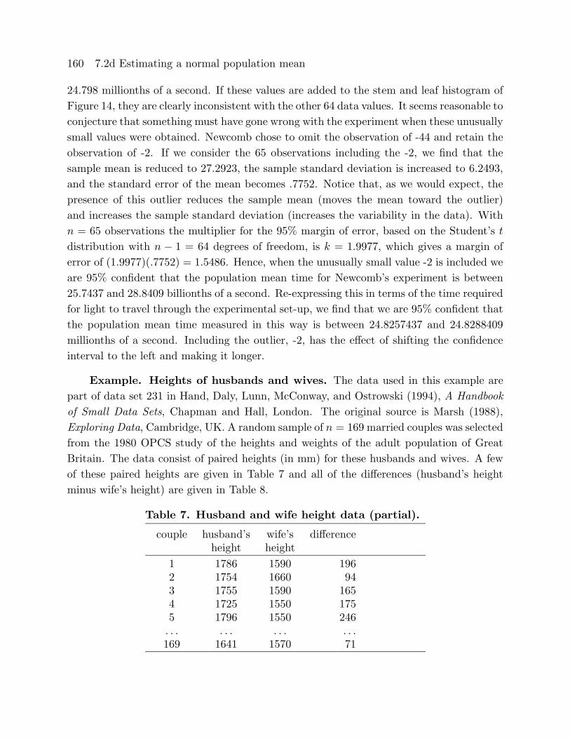
Example. Heights of husbands and wives. The data used in this example are
part of data set 231 in Hand, Daly, Lunn, McConway, and Ostrowski (1994), A Handbook
of Small Data Sets, Chapman and Hall, London. The original source is Marsh (1988),
Exploring Data, Cambridge, UK. A random sample of n = 169 married couples was selected
from the 1980 OPCS study of the heights and weights of the adult population of Great
Britain. The data consist of paired heights (in mm) for these husbands and wives. A few
of these paired heights are given in Table 7 and all of the differences (husband’s height
minus wife’s height) are given in Table 8.
Table 7. Husband and wife height data (partial).
couple husband’s wife’s differenceheight height
1 1786 1590 1962 1754 1660 943 1755 1590 1654 1725 1550 1755 1796 1550 246. . . . . . . . . . . .169 1641 1570 71
7.2d Estimating a normal population mean 161
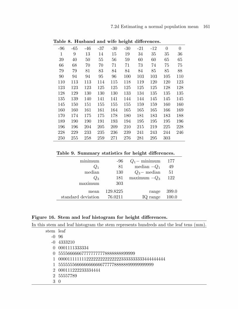
Table 8. Husband and wife height differences.
-96 -65 -46 -37 -30 -30 -21 -12 0 01 9 13 14 15 19 34 35 35 3639 40 50 55 56 59 60 60 65 6566 68 70 70 71 71 73 74 75 7579 79 81 83 84 84 84 85 85 8890 94 94 95 96 100 103 103 105 110110 113 113 114 115 118 119 120 120 123123 123 123 125 125 125 125 125 128 128128 129 130 130 130 133 134 135 135 135135 139 140 141 141 144 144 145 145 145145 150 151 155 155 155 159 159 160 160160 160 161 161 164 165 165 165 166 169170 174 175 175 178 180 181 183 183 188189 190 190 191 193 194 195 195 195 196196 196 204 205 209 210 215 219 225 228228 229 233 235 236 239 241 243 244 246250 255 258 259 271 276 281 295 303
Table 9. Summary statistics for height differences.
minimum -96 Q1− minimum 177Q1 81 median −Q1 49
median 130 Q3− median 51Q3 181 maximum −Q3 122
maximum 303
mean 129.8225 range 399.0standard deviation 76.0211 IQ range 100.0
Figure 16. Stem and leaf histogram for height differences.
In this stem and leaf histogram the stem represents hundreds and the leaf tens (mm).
stem leaf-0 96-0 43332100 00011113333340 5555666666777777777788888888999991 00001111111122222222222222233333333334444444441 555555566666666666677777888888999999999992 0001112222333344442 555577893 0

162 7.2d Estimating a normal population mean
Figure 17. Normal probability plot for height differences.
-100 0 100 200 300height difference
-3
-2
-1
0
1
2
3no
rmal
sco
re
Summary statistics for these differences are given in Table 9, a stem and leaf histogram
is provided in Figure 16, and a normal probability plot is given in Figure 17. Based on
the summary statistics, the stem and leaf histogram, and the normal probability plot it
seems reasonable to assume that these differences form a random sample from a normal
population of differences. The population mean difference µD is the average difference in
height corresponding to the population of all married couples in Great Britain in 1980.
(Technically, we should restrict this mean to those married couples included in the 1980
COPS study from which the sample was taken.)
The sample mean for these n = 169 differences is 129.8225 mm, the sample standard
deviation is 76.0211 mm, the standard error of the sample mean is 76.0211/√169 = 5.8478,
and the multiplier for the 95% margin of error, based on the Student’s t distribution with
n−1 = 168 degrees of freedom, is k = 1.9742. Thus the 95% margin of error of the samplemean is (1.9742)(5.8478) = 11.5447 and the limits for the 95% confidence interval estimate
of µD are 129.8225 − 11.5447 = 118.2778 and 129.8225 + 11.5447 = 141.3672. Therefore,we are 95% confident that for the population of all married couples in Great Britain in
1980, on average, the husband’s height exceeds the wife’s height by at least 118.2778 mm
and perhaps as much as 141.3672 mm.
Remark regarding directional confidence bounds. The use of one of the confidence
limits of a 90% confidence interval as a 95% confidence bound discussed in Section 5.4 can
also be used in the present context. That is, we can find an upper or lower 95% confidence
bound for µ by selecting the appropriate confidence limit from a 90% confidence interval
estimate of µ.
7.2e Tests of hypotheses about a normal population mean 163
7.2e Tests of hypotheses about a normal population mean
The hypothesis testing procedures discussed in this section are based on the fact that,
when µ = µ0, the Student’s t test statistic
Tcalc =X − µ0
S.E.(X)=
X − µ0
S/√n,
follows the Student’s t distribution with n − 1 degrees of freedom. Recall that, techni-cally, this result requires that the sample from which the sample mean X and the sample
standard deviation S are computed forms a random sample from a normal distribution
with population mean µ. However, these methods are known to be generally reasonable
even when the underlying population is not exactly a normal population, provided the
underlying population distribution is reasonably symmetric and the true density curve has
a more or less normal (bell–shaped) appearance. An alternate approach to inference (for
a population median) which may be used when the Student’s t methods are inappropriate
is discussed in Section 7.3.
Recall that a hypothesis (statistical hypothesis) is a conjecture about the nature of
the population. When we considered hypotheses about dichotomous populations we noted
that the population was completely determined by the population success proportion p. In
the present context of sampling from a normal population two parameters, the mean and
the standard deviation, must be specified to completely determine the normal population.
A hypothesis about the value of the population mean µ of a normal distribution specifies
where the center of this normal distribution, µ, is located on the number line but places
no restriction on the population standard deviation.
Even though the logic behind a hypothesis test for a population mean µ is the same
as the logic behind a hypothesis test for a population proportion p, we will introduce
hypothesis testing for a mean in the context of a simple hypothetical example.
Example. Strength of bricks. Consider a brick manufacturer that has produced
a large batch of bricks and wants to determine whether these bricks are suitable for a
particular construction project. The specifications for this project require bricks with a
mean compressive strength that exceeds 3200 psi. In order to assess the suitability of
this batch of bricks the manufacturer will obtain a simple random sample of bricks from
this batch and measure their compressive strength. In this example a single brick is a
unit, the entire large batch of bricks is the population, and a suitable variable X is the
compressive strength of an individual brick (in psi). We will assume that the distribution
of X is reasonably modeled by a normal distribution with population mean µ and popu-
lation standard deviation σ. In this example the population mean µ represents the mean

164 7.2e Tests of hypotheses about a normal population mean
compressive strength for all of the bricks in this large batch and the population standard
deviation quantifies the variability from brick to brick in (measured) compressive strength.
The manufacturer does not want to use these bricks for this construction project
unless there is sufficient evidence to claim that the population mean compressive strength
for this batch exceeds 3200 psi. Thus, the question of interest here is: “Is there sufficient
evidence to justify using this batch of bricks for this project?” In terms of the population
mean µ the research hypothesis is H1 : µ > 3200 (the mean compressive strength for this
batch of bricks exceeds 3200 psi); and the null hypothesis is H0 : µ ≤ 3200 (the meancompressive strength for this batch of bricks does not exceed 3200 psi). In other words,
the manufacturer will tentatively assume that these bricks are not suitable for this project
and will check to see if there is sufficient evidence against this tentative assumption to
justify the conclusion that these bricks are suitable for the project.
A test of the null hypothesis H0 : µ ≤ 3200 versus the research hypothesis H1 : µ >
3200 begins by tentatively assuming that the mean compressive strength for this batch of
bricks is no larger than 3200 psi. Under this tentative assumption it would be surprising
to observe a sample mean compressive strength X that was much larger than 3200. Thus
the test should reject H0 : µ ≤ 3200 in favor of H1 : µ > 3200 if the observed value of X is
sufficiently large relative to 3200. In order to determine whether X is large relative to 3200
we need an estimate of the sample to sample variability in X. The sample standard error
of the sample mean S.E.(X) = S/√n, where S denotes the sample standard deviation,
provides a suitable measure of the sample to sample variability in X. Our conclusion will
hinge on deciding whether the observed value of the Student’s t test statistic
Tcalc =X − 3200S.E.(X)
=X − 3200S/√n
is far enough above zero to make µ > 3200 more tenable than µ ≤ 3200. We will basethis decision on the probability of observing a value of T as large or larger than the
actual calculated value Tcalc of T , under the assumption that µ ≤ 3200. This probability(computed assuming that µ = 3200) is the P–value of the test. We will use the fact that,
when µ = 3200, the Student’s t statistic T follows the Student’s t distribution with n− 1degrees of freedom to calculate the P–value.
First suppose that a simple random sample of n = 100 bricks is selected from the
large batch. Further suppose that the sample mean compressive strength of these 100
bricks is X = 3481 psi and the sample standard deviation is S = 1118.38. In this case we
know that the mean compressive strength of the bricks in the sample X = 3481 exceeds
3200 and we need to decide whether this suggests that the mean compressive strength
of all of the bricks in the batch µ exceeds 3200. In this case the sample standard error
of X is S.E.(X) = 1118.38/√100 = 111.838. Thus X exceeds 3200 by 281 psi which is
7.2e Tests of hypotheses about a normal population mean 165
281/111.838 = 2.5126 standard error units, i.e., Tcalc = 2.5126. In this case the P–value
.0068 is the probability of observing a calculated T value as large or larger than 2.5126
when µ ≤ 3200. That is, if µ ≤ 3200 and we perform this experiment with n = 100,
then we would expect to see a value of X that is 2.5126 standard error units above the
hypothesized value 3200 (2.5126 times S.E.(X) psi above 3200) about 0.68% of the time.
Therefore, observing values of X and S in a sample of size n = 100 which yield a value of
Tcalc as large or larger than 2.5126 would be very surprising if the true mean compressive
strength for the batch µ was not larger than 3200 and we have sufficient evidence to reject
the null hypothesis H0 : µ ≤ 3200 in favor of the research hypothesis H1 : µ > 3200.
In the case we would conclude that there is sufficient evidence to contend that the mean
compressive strength for this batch of bricks exceeds 3200 psi, i.e., these bricks are suitable
for the construction project.
Now suppose that a simple random sample of n = 100 bricks is selected from the large
batch and the sample mean compressive strength of these 100 bricks is X = 3481 psi as
before. However, suppose that in this case the sample standard deviation is S = 2329.3. As
before we know that the mean compressive strength of the bricks in the sample X = 3481
exceeds 3200 and we need to decide whether this suggests that the mean compressive
strength of all of the bricks in the batch µ exceeds 3200. In this case the sample standard
error of X is S.E.(X) = 2329.3/√100 = 232.93. Thus X exceeds 3200 by 281 psi which
is 281/232.93 = 1.2064 standard error units, i.e., Tcalc = 1.2064. In this case the P–value
.1153 is the probability of observing a calculated T value as large or larger than 1.2064
when µ ≤ 3200. That is, if µ ≤ 3200 and we perform this experiment with n = 100, then wewould expect to see a value of X that is 1.2064 standard error units above the hypothesized
value 3200 (1.2064 times S.E.(X) psi above 3200) about 11.53% of the time. Therefore,
observing values of X and S in a sample of size n = 100 which yield a value of Tcalc as large
or larger than 1.2064 would not be very surprising if the true mean compressive strength
for the batch µ was not larger than 3200 and we do not have sufficient evidence to reject
the null hypothesis H0 : µ ≤ 3200 in favor of the research hypothesis H1 : µ > 3200. In
the case we would conclude that there is not sufficient evidence to contend that the mean
compressive strength for this batch of bricks exceeds 3200 psi, i.e., these bricks are not
suitable for the construction project.
The research hypothesis in the brick example is a directional hypothesis of the form
H1 : µ > µ0, where µ0 = 3200. We will now discuss the details of a hypothesis test
for a directional research hypothesis of this form. For the test procedure to be valid the
specified value µ0 and the direction of the research hypothesis must be motivated from
subject matter knowledge before looking at the data that are to be used to perform the
test.
166 7.2e Tests of hypotheses about a normal population mean
Let µ0 denote the hypothesized value which we wish to compare with µ. The research
hypothesis states that µ is greater than µ0; in symbols we will indicate this research
hypothesis by writing
H1 : µ > µ0.
The null hypothesis is the negation of H1 : µ > µ0 which states that µ is not greater than
µ0; in symbols we will indicate this null hypothesis by writing
H0 : µ ≤ µ0.
The research hypothesis H1 : µ > µ0 specifies that the normal distribution is one of the
normal distributions for which the population mean µ is greater than µ0. The null hypoth-
esis H0 : µ ≤ µ0 specifies that the normal distribution is one of the normal distributions
for which the population mean µ is at most µ0. The population standard deviation σ is
not restricted by either hypothesis. Assuming that the population standard deviation is
the same regardless of which hypothesis is true, this competing pair of hypotheses provides
a decomposition of all possible normal distributions with this σ into the collection of nor-
mal distributions where µ > µ0 and the research hypothesis is true and the collection of
normal distributions where µ ≤ µ0 and the null hypothesis is true. Our goal is to use the
data to decide which of these two collections of normal distributions contains the normal
distribution we are actually sampling from.
Since a hypothesis test begins by tentatively assuming that the null hypothesis is
true, we need to decide what constitutes evidence against the null hypothesis H0 : µ ≤ µ0
and in favor of the research hypothesis H1 : µ > µ0. We will assume that the unknown
population standard deviation σ is fixed regardless of the value of µ. The difference X−µ0
between the sample mean X and the hypothesized value µ0, expressed in standard error
units, will be used to assess the strength of the evidence in favor of the research hypothesis.
Generally, we would expect to observe larger values of X more often when the research
hypothesis H1 : µ > µ0 is true than when the null hypothesis H0 : µ ≤ µ0 is true. In
particular, we can view the observation of a value of X that is sufficiently large relative
to µ0 as constituting evidence against the null hypothesis H0 : µ ≤ µ0 and in favor of the
research hypothesis H1 : µ > µ0. To decide whether the observed value of X is “sufficiently
large relative to µ0” we need to take the variability in the data into account. We can do
this by basing our decision on the corresponding Student’s t test statistic,
Tcalc =X − µ0
S.E.(X)=
X − µ0
S/√n,
instead of X alone. Notice that values of Tcalc which are large relative to zero correspond
to values of X which are large relative to µ0. Deciding whether the observed value of Tcalc
7.2e Tests of hypotheses about a normal population mean 167
is sufficiently large relative to zero to allow rejection of H0 is based on the corresponding
P–value, which is defined below.
The P–value for testing the null hypothesis H0 : µ ≤ µ0 versus the research hypothesis
H1 : µ > µ0 is the probability of observing a value of a Student’s t variable T as large or
larger than the calculated value Tcalc that we actually do observe, i.e., P–value = P (T ≥Tcalc), where T denotes a Student’s t variable with n−1 degrees of freedom. This P–valueis computed under the assumption that the research hypothesis H1 : µ > µ0 is false and
the null hypothesis H0 : µ ≤ µ0 is true. Because the null hypothesis only specifies that
µ ≤ µ0, we need to choose a particular value of µ (that is no larger than µ0) in order to
compute the P–value. It is most appropriate to use µ = µ0 for this computation. Using
µ = µ0, which defines the boundary between µ ≤ µ0, where the null hypothesis is true, and
µ > µ0, where the research hypothesis is true, provides some protection against incorrectly
rejecting H0 : µ ≤ µ0.
The steps for performing a hypothesis test for
H0 : µ ≤ µ0 versus H1 : µ > µ0
are summarized below.
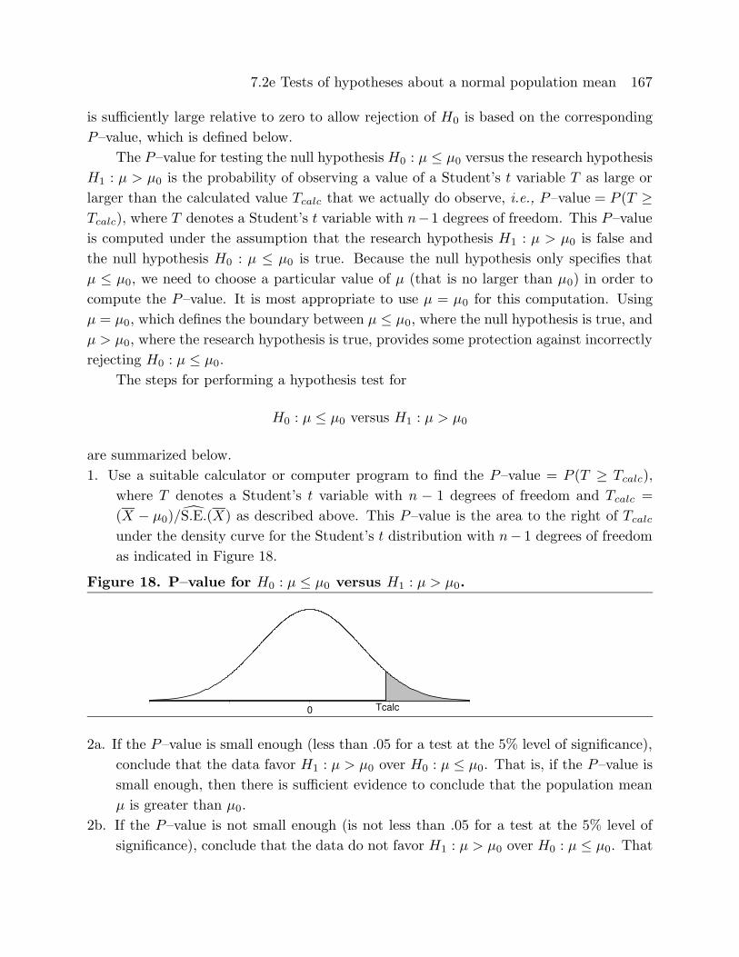
1. Use a suitable calculator or computer program to find the P–value = P (T ≥ Tcalc),
where T denotes a Student’s t variable with n − 1 degrees of freedom and Tcalc =
(X − µ0)/S.E.(X) as described above. This P–value is the area to the right of Tcalc
under the density curve for the Student’s t distribution with n− 1 degrees of freedomas indicated in Figure 18.
Figure 18. P–value for H0 : µ ≤ µ0 versus H1 : µ > µ0.
0 Tcalc
2a. If the P–value is small enough (less than .05 for a test at the 5% level of significance),
conclude that the data favor H1 : µ > µ0 over H0 : µ ≤ µ0. That is, if the P–value is
small enough, then there is sufficient evidence to conclude that the population mean
µ is greater than µ0.
2b. If the P–value is not small enough (is not less than .05 for a test at the 5% level of
significance), conclude that the data do not favor H1 : µ > µ0 over H0 : µ ≤ µ0. That
168 7.2e Tests of hypotheses about a normal population mean
is, if the P–value is not small enough, then there is not sufficient evidence to conclude
that the population mean µ is greater than µ0.
The procedure for testing the null hypothesis H0 : µ ≤ µ0 versus the research hypoth-
esis H1 : µ > µ0 given above is readily modified for testing the null hypothesis H0 : µ ≥ µ0
versus the research hypothesis H1 : µ < µ0. The essential modification is to change the
direction of the inequality in the definition of the P–value. Consider a situation where
the research hypothesis specifies that the population mean µ is less than the particular,
hypothesized value µ0. For these hypotheses values of the sample mean X that are suffi-
ciently small relative to µ0 provide evidence in favor of the research hypothesis H1 : µ < µ0
and against the null hypothesis H0 : µ ≥ µ0. Therefore, the appropriate P–value is the
probability of observing a value of a Student’s t variable T as small or smaller than the
value actually observed. As before, the P–value is computed under the assumption that
µ = µ0. The calculated t statistic Tcalc is defined as before; however, in this situation
the P–value is the area under the density curve of the Student’s t distribution with n− 1degrees of freedom to the left of Tcalc, since values of X that are small relative to µ0
constitute evidence in favor of the research hypothesis.
The steps for performing a hypothesis test for
H0 : µ ≥ µ0 versus H1 : µ < µ0
are summarized below.
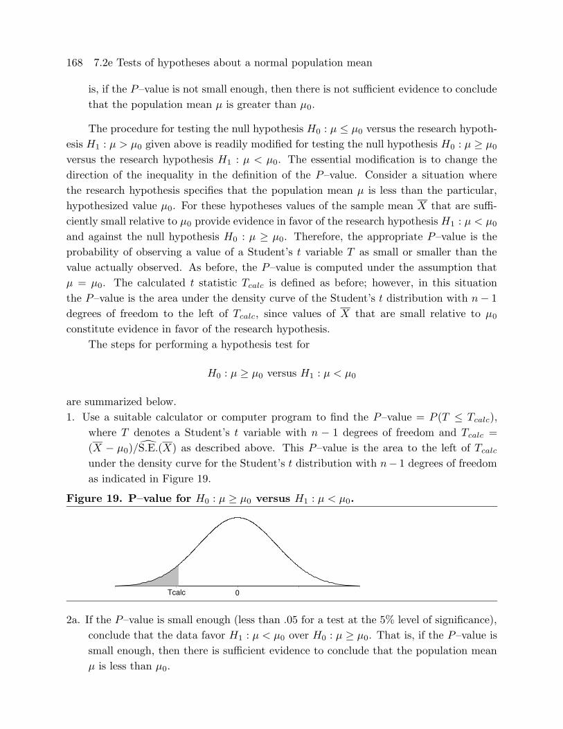
1. Use a suitable calculator or computer program to find the P–value = P (T ≤ Tcalc),
where T denotes a Student’s t variable with n − 1 degrees of freedom and Tcalc =
(X − µ0)/S.E.(X) as described above. This P–value is the area to the left of Tcalc
under the density curve for the Student’s t distribution with n− 1 degrees of freedomas indicated in Figure 19.
Figure 19. P–value for H0 : µ ≥ µ0 versus H1 : µ < µ0.
Tcalc 0
2a. If the P–value is small enough (less than .05 for a test at the 5% level of significance),
conclude that the data favor H1 : µ < µ0 over H0 : µ ≥ µ0. That is, if the P–value is
small enough, then there is sufficient evidence to conclude that the population mean
µ is less than µ0.

7.2e Tests of hypotheses about a normal population mean 169
2b. If the P–value is not small enough (is not less than .05 for a test at the 5% level of
significance), conclude that the data do not favor H1 : µ < µ0 over H0 : µ ≥ µ0. That
is, if the P–value is not small enough, then there is not sufficient evidence to conclude
that the population mean µ is less than µ0.
Example. Brain changes in response to experience. A study by Rosenzweig,
Bennett, and Diamond, described in an article in Scientific American (1964), was con-
ducted to examine the effects of psychological environment on the anatomy of the brain.
The units for this study came from a strain of genetically pure rats. A pair of rats was
selected at random from each of 12 litters of rats; one of these rats was placed in group
A and the other in group B. Each animal in group A lived with eleven others in a large
cage, furnished with playthings which were changed daily. Each animal in group B lived
in isolation, with no toys. Both groups of rats were provided with as much food and drink
as they desired. After a month, the rats were killed and dissected. One variable which
was measured was the weight (in milligrams) of the cortex of the rat. The cortex is the
“thinking” part of the brain. The question we wish to address here is whether there is
evidence in favor of the contention that the cortex of a rat raised in the more stimulating
environment of group A will tend to be larger than the cortex of a rat raised in the less
stimulating environment of group B.
The researchers conducted this experiment five times. Data from one of these exper-
iments are given in Table 10. There are sets of three values for each of twelve pairs of
littermates in this table: the weight of the cortex of the rat in group A, the weight of the
cortex of the rat in group B, and the difference between these two weights (A weight minus
B weight); all of these values are measured in milligrams.
Table 10. Rat cortex weight data.
pair group A group B difference pair group A group B difference
1 690 668 22 7 720 665 552 701 667 34 8 718 689 293 685 647 38 9 718 642 764 751 693 58 10 696 673 235 647 635 12 11 658 675 -176 647 644 3 12 680 641 39
Summary statistics for the differences in cortex weights (A weight minus B weight)
are given in Table 11, a stem and leaf histogram is provided in Figure 20, and a normal
probability plot is given in Figure 21. Based on the summary statistics and the stem
and leaf histogram there is some evidence that this distribution is slightly skewed to the
left; however, the normal probability plot is reasonably linear and it seems reasonable to
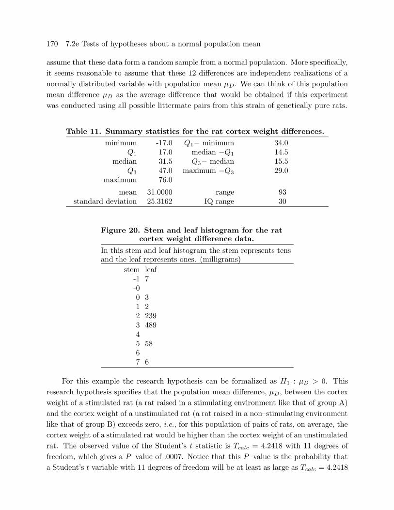
170 7.2e Tests of hypotheses about a normal population mean
assume that these data form a random sample from a normal population. More specifically,
it seems reasonable to assume that these 12 differences are independent realizations of a
normally distributed variable with population mean µD. We can think of this population
mean difference µD as the average difference that would be obtained if this experiment
was conducted using all possible littermate pairs from this strain of genetically pure rats.
Table 11. Summary statistics for the rat cortex weight differences.
minimum -17.0 Q1− minimum 34.0Q1 17.0 median −Q1 14.5
median 31.5 Q3− median 15.5Q3 47.0 maximum −Q3 29.0
maximum 76.0
mean 31.0000 range 93standard deviation 25.3162 IQ range 30
Figure 20. Stem and leaf histogram for the ratcortex weight difference data.
In this stem and leaf histogram the stem represents tensand the leaf represents ones. (milligrams)
stem leaf-1 7-00 31 22 2393 48945 5867 6
For this example the research hypothesis can be formalized as H1 : µD > 0. This
research hypothesis specifies that the population mean difference, µD, between the cortex
weight of a stimulated rat (a rat raised in a stimulating environment like that of group A)
and the cortex weight of a unstimulated rat (a rat raised in a non–stimulating environment
like that of group B) exceeds zero, i.e., for this population of pairs of rats, on average, the
cortex weight of a stimulated rat would be higher than the cortex weight of an unstimulated
rat. The observed value of the Student’s t statistic is Tcalc = 4.2418 with 11 degrees of
freedom, which gives a P–value of .0007. Notice that this P–value is the probability that
a Student’s t variable with 11 degrees of freedom will be at least as large as Tcalc = 4.2418
7.2e Tests of hypotheses about a normal population mean 171
when µD = 0. Since this P–value is quite small, there is very strong evidence that the
population mean difference µD is greater than zero. Hence, the data do support the
contention that for this population of pairs of rats, on average, the cortex weight of a
stimulated rat would be higher than the cortex weight of an unstimulated rat.
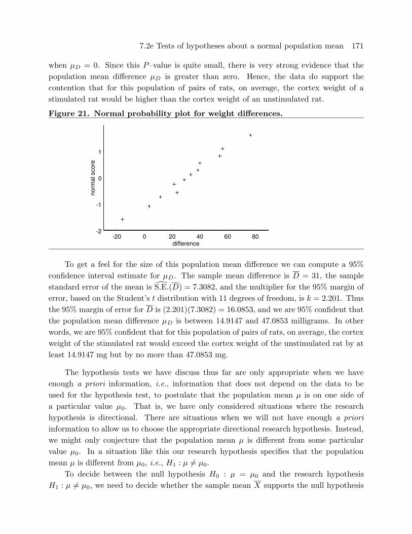
Figure 21. Normal probability plot for weight differences.
-20 0 20 40 60 80difference
-2
-1
0
1
norm
al s
core
To get a feel for the size of this population mean difference we can compute a 95%
confidence interval estimate for µD. The sample mean difference is D = 31, the sample
standard error of the mean is S.E.(D) = 7.3082, and the multiplier for the 95% margin of
error, based on the Student’s t distribution with 11 degrees of freedom, is k = 2.201. Thus
the 95% margin of error for D is (2.201)(7.3082) = 16.0853, and we are 95% confident that
the population mean difference µD is between 14.9147 and 47.0853 milligrams. In other
words, we are 95% confident that for this population of pairs of rats, on average, the cortex
weight of the stimulated rat would exceed the cortex weight of the unstimulated rat by at
least 14.9147 mg but by no more than 47.0853 mg.
The hypothesis tests we have discuss thus far are only appropriate when we have
enough a priori information, i.e., information that does not depend on the data to be
used for the hypothesis test, to postulate that the population mean µ is on one side of
a particular value µ0. That is, we have only considered situations where the research
hypothesis is directional. There are situations when we will not have enough a priori
information to allow us to choose the appropriate directional research hypothesis. Instead,
we might only conjecture that the population mean µ is different from some particular
value µ0. In a situation like this our research hypothesis specifies that the population
mean µ is different from µ0, i.e., H1 : µ 6= µ0.
To decide between the null hypothesis H0 : µ = µ0 and the research hypothesis
H1 : µ 6= µ0, we need to decide whether the sample mean X supports the null hypothesis
172 7.2e Tests of hypotheses about a normal population mean
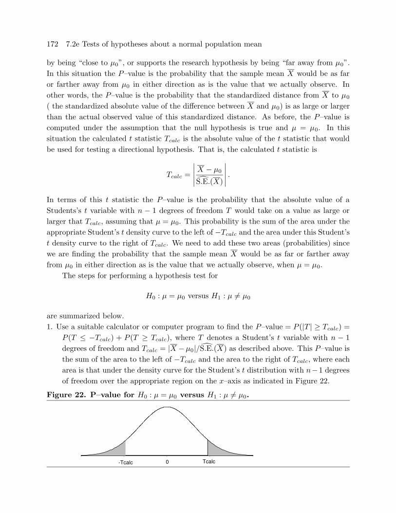
by being “close to µ0”, or supports the research hypothesis by being “far away from µ0”.
In this situation the P–value is the probability that the sample mean X would be as far
or farther away from µ0 in either direction as is the value that we actually observe. In
other words, the P–value is the probability that the standardized distance from X to µ0
( the standardized absolute value of the difference between X and µ0) is as large or larger
than the actual observed value of this standardized distance. As before, the P–value is
computed under the assumption that the null hypothesis is true and µ = µ0. In this
situation the calculated t statistic Tcalc is the absolute value of the t statistic that would
be used for testing a directional hypothesis. That is, the calculated t statistic is
Tcalc =
∣∣∣∣∣X − µ0
S.E.(X)
∣∣∣∣∣ .
In terms of this t statistic the P–value is the probability that the absolute value of a
Students’s t variable with n − 1 degrees of freedom T would take on a value as large or
larger that Tcalc, assuming that µ = µ0. This probability is the sum of the area under the
appropriate Student’s t density curve to the left of −Tcalc and the area under this Student’s
t density curve to the right of Tcalc. We need to add these two areas (probabilities) since
we are finding the probability that the sample mean X would be as far or farther away
from µ0 in either direction as is the value that we actually observe, when µ = µ0.
The steps for performing a hypothesis test for
H0 : µ = µ0 versus H1 : µ 6= µ0
are summarized below.
1. Use a suitable calculator or computer program to find the P–value = P (|T | ≥ Tcalc) =
P (T ≤ −Tcalc) + P (T ≥ Tcalc), where T denotes a Student’s t variable with n − 1degrees of freedom and Tcalc = |X −µ0|/S.E.(X) as described above. This P–value isthe sum of the area to the left of −Tcalc and the area to the right of Tcalc, where each
area is that under the density curve for the Student’s t distribution with n−1 degreesof freedom over the appropriate region on the x–axis as indicated in Figure 22.
Figure 22. P–value for H0 : µ = µ0 versus H1 : µ 6= µ0.
Tcalc-Tcalc 0
7.2e Tests of hypotheses about a normal population mean 173
2a. If the P–value is small enough (less than .05 for a test at the 5% level of significance),
conclude that the data favor H1 : µ 6= µ0 over H0 : µ = µ0. That is, if the P–value is
small enough, then there is sufficient evidence to conclude that the population mean
µ is not equal to µ0.
2b. If the P–value is not small enough (is not less than .05 for a test at the 5% level of
significance), conclude that the data do not favor H1 : µ 6= µ0 over H0 : µ = µ0. That
is, if the P–value is not small enough, then there is not sufficient evidence to conclude
that the population mean µ differs from µ0.
Example. Newcomb’s measurements of the speed of light (revisited). The
parameter we were estimating in our analysis of Newcomb’s measurements of the speed of
light was the population mean time µ for light to travel a distance of 7442 meters. Notice
that the population mean time µ is actually defined by the process of measurement being
used. That is, we can think of µ as the long run average time that we would observe if
we replicated Newcomb’s experiment a large times. We might wonder how this population
mean time µ relates to the “true time” it would take for light to travel a distance of
7442 meters. We don’t know exactly what this “true time” is, but we can use a generally
accepted, modern measurement of the speed of light to obtain a hypothesized “true time.”
Stigler (op. cit.) used the modern estimate of the speed of light in a vacuum of 299,792.5
km/sec adjusted to give the speed of light in air and converted to a time as measured by
Newcomb to obtain a hypothesized “true time” of 33.02. Therefore, our present goal is to
determine how the population mean time µ relates to the “true time” µ0 = 33.02.
We do not have sufficient a priori information to specify a directional hypothesis;
therefore, we will test the null hypothesis H0 : µ = 33.02 versus the research hypothesis
H1 : µ 6= 33.02 to determine whether the population mean time µ is equal to or differentfrom the hypothesized “true value” of 33.02. For Newcomb’s n = 64 measurements the
sample mean is X = 27.75, the sample standard error of the mean is S.E.(X) = .6354, and
the calculated t statistic is
Tcalc =
∣∣∣∣27.75− 33.02
.6354
∣∣∣∣ = 8.2940.
The P–value is less than .0001 indicating that observing a sample mean as far away from
the hypothesized “true value” 33.02 (in either direction) as Newcomb did is extremely
unlikely if in fact µ = 33.02. We can conclude that the population mean µ corresponding
to Newcomb’s experiment is almost certainly not equal to the hypothesized value of 33.02.
The confidence interval, (26.4803, 29.0197), we computed above suggests that the mean µ
that Newcomb was estimating is less than the hypothesized value 33.02.
174 7.3 Inference for a population median
7.3 Inference for a population median
The inferential methods for a population mean discussed above require at least ap-
proximate normality of the population distribution of the variable of interest. In this
section we will consider methods for making inferences about a population median which
do not require the assumption of a particular form for the population distribution of the
variable of interest. That is, the inferential methods considered in this section are appli-
cable for any population distribution for a continuous variable regardless of the shape of
the corresponding density curve.
We will begin by discussing a method for testing a hypothesis about a population
median. The essence of this method is to re–express the hypothesis about the population
median as a hypothesis about a related population proportion and to then use inferential
methods for a population proportion to test the hypothesis about the population median.
For a continuous variable X we can think of the population medianM as the point on
the number line which divides the area under the corresponding population density curve
into two equal areas (each of area one–half). The population median M is analogous to
the sample median which divides the histogram into two equal areas. Notice that if we
observe a single value of X, then the probability that we will observe a value larger than
the population median M is 1/2, i.e., P (X > M) = 1/2, and similarly, the probability
that we will observe a value smaller than M is 1/2, i.e., P (X < M) = 1/2.
Let M denote the population median of the distribution of the continuous variable X
and consider a hypothesis relating the population median M to a particular, fixed value
M0. We can dichotomize the population of values of X by thinking of the event “observe
X > M0” as a success and the event “observe X < M0” as a failure. The population
success proportion p corresponding to this dichotomization is p = P (X > M0), i.e., p is
the probability that a single value of X chosen from the infinite population of values of
X will be larger than the hypothesized value M0. The corresponding population failure
proportion is 1− p = P (X < M0).
The three possible relationships between the population median M and the partic-
ular value M0 are readily re–expressed in terms of the corresponding population suc-
cess probability p = P (X > M0). If the population median M exceeds the partic-
ular value M0, then, since the area or probability to the right of the population me-
dian M is 1/2 and since M0 is to the left of M on the number line, we must have
p = P (X > M0) > 1/2 = P (X > M). Hence we see that M > M0 is equivalent to
p > 1/2. Similarly, if M is less than M0, then M0 is to the right of M on the number line
and we must have p = P (X > M0) < 1/2 = P (X > M); thus M < M0 is equivalent to
p < 1/2. Finally, if M = M0, then we must have p = P (X > M0) = 1/2 = P (X > M);
thus M = M0 is equivalent to p = 1/2. These relationships allow us to re–express a
7.3 Inference for a population median 175
hypothesis relating the population median M to the particular value M0 as a hypothesis
about the corresponding population success probability p = P (X > M0).
For ease of reference the three standard pairs of null and research hypotheses about
M are summarized below (recall that p = P (X > M0))
1. H0 :M ≤M0 versus H1 :M > M0 corresponds to H0 : p ≤ .5 versus H1 : p > .5.
2. H0 :M ≥M0 versus H1 :M < M0 corresponds to H0 : p ≥ .5 versus H1 : p < .5.
3. H0 :M =M0 versus H1 :M 6=M0 corresponds to H0 : p = .5 versus H1 : p 6= .5.
The dichotomy described above, where X > M0 constitutes a success and X < M0
constitutes a failure, does not allow for the possibility that the continuous variable X
is exactly equal to M0. This is allowable, theoretically, when we are talking about the
population distribution of X; however, when we examine the data we may find that one or
more of the observations are equal to the hypothesized value M0. The easiest solution to
this potential difficulty is to remove any observations which are exactly equal to M0 and
adjust the sample size accordingly before we perform a hypothesis test. In other words,
a hypothesis test for comparing the population median M to the hypothesized value M0
is based on the observed proportion p of successes (values of X which are greater than
M0) relative to n, where n is the number of observations which are not equal to M0. An
alternative to discarding values exactly equal to M0 is to classify half of these values as
successes and half as failures and use the original sample size for n.
Example. Darwin’s plant height comparison. Charles Darwin conducted an
experiment to determine whether cross–fertilized plants tend to be more vigorous than self–
fertilized plants. (The plants used in Darwin’s study were young corn (Zea mays) plants.)
(Darwin (1876), The Effect of Cross– and Self–fertilization in the Vegetable Kingdom,
second edition, John Murray, London) Darwin selected several plants and fertilized several
flowers on each plant; a number of flowers were cross–fertilized with pollen taken from
distant plants and a number of flowers were self–fertilized with their own pollen. Seeds
gathered from these flowers were allowed to ripen and were then placed in wet sand to
germinate. Fifteen seedlings from cross–fertilized seeds were selected and fifteen seedlings
from self–fertilized seeds were selected. These seedlings were paired (one cross–fertilized
and one self–fertilized) and the two seedlings in each pair were planted on opposite sides of
the same pot. After a fixed period of time the height of each plant (in inches) was recorded.
The raw data and the associated differences are provided in Table 12. The distribution of

176 7.3 Inference for a population median
the differences is summarized in Table 13 and Figure 23 and a normal probability plot is
given in Figure 24.
Table 12. Plant height data.
plant height
pair cross–fertilized self–fertilized difference
1 23.500 17.375 6.1252 12.000 20.375 -8.3753 21.000 20.000 1.0004 22.000 20.000 2.0005 19.125 18.375 0.7506 21.500 18.625 2.8757 22.125 18.625 3.5008 20.375 15.250 5.1259 18.250 16.500 1.75010 21.625 18.000 3.62511 23.250 16.250 7.00012 21.000 18.000 3.00013 22.125 12.750 9.37514 23.000 15.500 7.50015 12.000 18.000 -6.000
If it is true that cross–fertilized plants tend to be more vigorous than self–fertilized
plants, then we would expect a cross–fertilized plant to be taller than a self–fertilized plant
of the same age. Therefore, we can formalize this theory as the research hypothesis that
the population median of the difference between the height of a cross–fertilized plant and
the height of a self–fertilized plant grown in the same pot MD is greater than zero, i.e.,
H1 :MD > 0. We can think of the population as consisting of all of the pairs of seedlings
(one cross–fertilized and one self–fertilized) which could have been used in this experiment;
and, we can think of the population median differenceMD as the median of the differences
between the heights of these pairs of seedlings (height of the cross–fertilized plant minus
height of the self–fertilized plant). Notice that this research hypothesis specifies that, for
this population of potential pairs of plants, the cross-fertilized plant would be taller than
the self–fertilized plant more than half of the time.
Table 13. Summary statistics for the plant height differences.
minimum -8.375 Q1− minimum 9.375Q1 1.000 median −Q1 4.000
median 3.000 Q3− median 3.125Q3 6.125 maximum −Q3 3.250
maximum 9.375
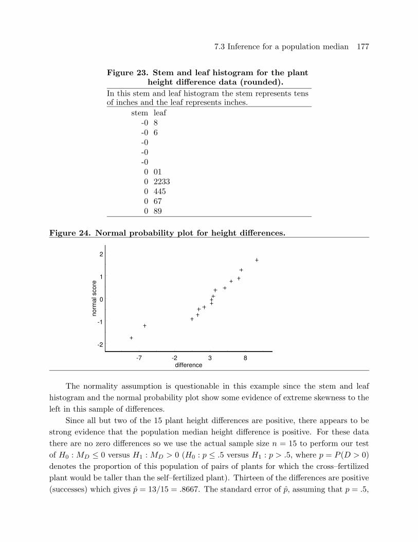
7.3 Inference for a population median 177
Figure 23. Stem and leaf histogram for the plantheight difference data (rounded).
In this stem and leaf histogram the stem represents tensof inches and the leaf represents inches.
stem leaf-0 8-0 6-0-0-00 010 22330 4450 670 89
Figure 24. Normal probability plot for height differences.
-7 -2 3 8difference
-2
-1
0
1
2
norm
al s
core
The normality assumption is questionable in this example since the stem and leaf
histogram and the normal probability plot show some evidence of extreme skewness to the
left in this sample of differences.
Since all but two of the 15 plant height differences are positive, there appears to be
strong evidence that the population median height difference is positive. For these data
there are no zero differences so we use the actual sample size n = 15 to perform our test
of H0 :MD ≤ 0 versus H1 :MD > 0 (H0 : p ≤ .5 versus H1 : p > .5, where p = P (D > 0)
denotes the proportion of this population of pairs of plants for which the cross–fertilized
plant would be taller than the self–fertilized plant). Thirteen of the differences are positive
(successes) which gives p = 13/15 = .8667. The standard error of p, assuming that p = .5,
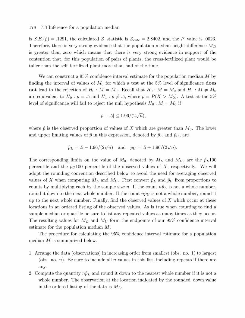
178 7.3 Inference for a population median
is S.E.(p) = .1291, the calculated Z–statistic is Zcalc = 2.8402, and the P–value is .0023.
Therefore, there is very strong evidence that the population median height difference MD
is greater than zero which means that there is very strong evidence in support of the
contention that, for this population of pairs of plants, the cross-fertilized plant would be
taller than the self–fertilized plant more than half of the time.
We can construct a 95% confidence interval estimate for the population median M by
finding the interval of values of M0 for which a test at the 5% level of significance does
not lead to the rejection of H0 : M = M0. Recall that H0 : M = M0 and H1 : M 6= M0
are equivalent to H0 : p = .5 and H1 : p 6= .5, where p = P (X > M0). A test at the 5%
level of significance will fail to reject the null hypothesis H0 :M =M0 if
|p− .5| ≤ 1.96/(2√n),
where p is the observed proportion of values of X which are greater than M0. The lower
and upper limiting values of p in this expression, denoted by pL and pU , are
pL = .5− 1.96/(2√n) and pU = .5 + 1.96/(2
√n).
The corresponding limits on the value of M0, denoted by ML and MU , are the pL100
percentile and the pU100 percentile of the observed values of X, respectively. We will
adopt the rounding convention described below to avoid the need for averaging observed
values of X when computing ML and MU . First convert pL and pU from proportions to
counts by multiplying each by the sample size n. If the count npL is not a whole number,
round it down to the next whole number. If the count npU is not a whole number, round it
up to the next whole number. Finally, find the observed values of X which occur at these
locations in an ordered listing of the observed values. As is true when counting to find a
sample median or quartile be sure to list any repeated values as many times as they occur.
The resulting values for ML and MU form the endpoints of our 95% confidence interval
estimate for the population median M .
The procedure for calculating the 95% confidence interval estimate for a population
median M is summarized below.
1. Arrange the data (observations) in increasing order from smallest (obs. no. 1) to largest
(obs. no. n). Be sure to include all n values in this list, including repeats if there are
any.
2. Compute the quantity npL and round it down to the nearest whole number if it is not a
whole number. The observation at the location indicated by the rounded–down value
in the ordered listing of the data is ML.
7.4 Summary 179
3. Compute the quantity npU and round it up to the nearest whole number if it is not a
whole number. The observation at the location indicated by the rounded–up value in
the ordered listing of the data is MU .
4. Conclude that we are 95% confident that the population median M is between ML and
MU .
Example. Darwin’s plant height comparison (revisited). For this example
we have 1.96/(2√15) = .2530, pL = .5 − .2530 = .2470, and pU = .5 + .2530 = .7530,
giving npL = 3.705 which we round down to 3 and npU = 11.295 which we round up to
12. Observation number 3 is .75 and observation number 12 is 6.125. Therefore, we are
95% confident that the population median height difference for this population of pairs of
plants is between .75 inches and 6.125 inches.
7.4 Summary
The majority of this chapter is devoted to inference for the population mean µ of the
distribution of a continuous variable X. We began by discussing probability models for
the distribution of a continuous variable (density curves) and then introduced the normal
distribution which serves as the basis for our inferences about µ (based on the Student’s t
distribution).
Given data which form a random sample of size n from a population with population
mean µ and population standard deviation σ, the sampling distribution of the sample
mean X has mean µ and the population standard error of X is S.E.(X) = σ/n. Thus the
sample mean X is unbiased as an estimator of the population mean µ and the variability
in the sample mean X as an estimator of the population mean µ can be quantified by
this standard error. If we also assume that the population distribution of X is a normal
distribution, i.e., if we assume that the data form a random sample of size n from a
normal distribution with population mean µ and population standard deviation σ, then
the sampling distribution of X is the normal distribution with population mean µ (the
same as that of X) and standard deviation S.E.(X).
Given data which form a random sample of size n from a normal distribution with
population mean µ and population standard deviation σ and with sample mean X and
sample standard deviation SX = S, the quantity
T =X − µ
S/√n
follows the Student’s t distribution with n − 1 degrees of freedom. Therefore, if the as-sumption that the population distribution of X is normal is reasonable, then we can use
the Student’s t distribution to make inferences about the population mean µ. It is im-
portant to remember the normality assumption needed for the Student’s t distribution
180 7.5 Exercises
and to verify that this assumption is reasonable by examining the data for violations of
this assumption. The Student’s t methods work reasonably well provided the normality
assumption is not totally unreasonable.
The interval from X − kS/√n to X + kS/
√n, where k denotes the 97.5 percentile of
the Student’s t distribution with n− 1 degrees of freedom, is a 95% confidence interval forµ. We can test a hypothesis relating µ to a specified value µ0 by using the Student’s t test
statistic
Tcalc =X − µ0
S/√n
to find the appropriate P–value. The P–value for H1 : µ > µ0 is the probability P (T ≥Tcalc); the P–value for H1 : µ < µ0 is the probability P (T ≤ Tcalc); and, the P–value for
H1 : µ 6= µ0 is the probability P (|T | ≥ |Tcalc|), where T denotes a Student’s t variablewith n−1 degrees of freedom, i.e., these P–values are areas under the density curve of theStudent’s t distribution with n− 1 degrees of freedom.
The Student’s t inferential methods for a population mean are based on the assumption
that the underlying population distribution is reasonably modeled by a normal distribution.
When this normality assumption is not tenable we need to consider a method of inference
which is applicable under weaker assumptions. One approach to inference about the center
of a distribution based on the population median is discussed in Section 7.4. This approach
to inference about the population median does not require the assumption of a specific form
for the underlying population distribution.
7.5 Exercises
Provide a complete analysis for the following example. Be sure to: define a relevant popu-
lation mean µ; setup and perform a relevant hypothesis test; and, find a confidence interval
for µ. Be sure to include comments regarding the validity of the normality assumption for
this example. Provide a complete summary of your findings in the context of the example.
1. An article by Rosner, Willett, and Spiegelman in Statistics in Medicine (1989) describes
a study conducted to assess the make up of the diets of a population of women. The data
used here are as reported in Ott and Longnecker (2002). A sample of n = 168 women
was obtained and each of these women completed a food frequency questionnaire. The
completed questionnaires were then used to determine the percentage of calories from fat
in each woman’s diet. The values of the variable X, the percentage of calories from fat in
a woman’s diet, are summarized in the stem and leaf histogram in Figure 25. For display
purposes the data have been rounded to the nearest 1 percent. The actual data are given
in Table 14. In 2002 the Food and Nutrition Board, a unit of the Institute of Medicine
iom.edu, recommended that adults should restrict the percentage of calories from fat in
their diet to the range from 20% to 35%.

7.5 Exercises 181
If you wish to analyze these data without entering all n = 168 values in your computer
or calculator you may use the facts that: the sample mean for these data is 36.91899 and
the sample standard deviation is 6.72820.
Figure 25. Stem and leaf histogram for percentage of calories from fat.
In this stem and leaf histogram the stem represents tens and the leaf representsones. For example, the smallest value is 16% and the largest is 58%.
stem leaf11 62 0142 556666778889999993 0000011111112222222223333333344444444443 55555555555556666666666667777778888888888889999999994 00000000011111111112222222223344444444 5556666678885 001345 68
Table 14. Percentage of calories from fat data.
15.92 20.22 20.80 24.06 24.98 25.07 25.53 26.16 26.18 26.2726.79 27.29 27.54 28.16 28.35 28.76 29.07 29.34 29.34 29.4529.46 29.55 29.72 29.94 29.99 30.50 30.61 30.71 30.96 30.9931.02 31.10 31.27 31.61 31.71 31.75 31.97 32.24 32.26 32.2832.43 32.73 32.86 32.96 33.08 33.11 33.13 33.23 33.32 33.5133.71 33.72 33.86 33.87 33.95 34.11 34.17 34.25 34.31 34.5134.86 34.87 34.87 34.89 35.09 35.18 35.18 35.20 35.29 35.3235.49 35.50 35.56 35.67 35.69 35.71 35.74 35.77 36.07 36.0736.30 36.32 36.32 36.37 36.58 37.04 37.10 37.14 37.34 37.3937.47 37.56 37.85 37.88 37.89 38.02 38.04 38.10 38.19 38.2138.36 38.41 38.45 38.58 38.81 38.88 38.89 38.97 39.13 39.2239.25 39.40 39.80 39.84 39.95 40.05 40.12 40.25 40.29 40.4640.48 40.69 41.12 41.15 41.22 41.29 41.30 41.32 41.41 41.4241.44 41.53 41.64 41.69 41.78 41.89 42.12 42.17 42.20 42.3742.60 42.98 43.57 43.74 43.79 44.27 44.28 44.33 44.39 44.6645.06 45.28 45.51 45.82 45.83 46.22 46.38 46.97 47.63 47.8348.29 49.65 49.86 50.72 53.08 54.05 55.54 57.85

182 7.5 Exercises
2. Cox and Snell (1981), Applied Statistics, Chapman and Hall, discuss a study conducted
to examine changes in blood pressure due to the drug captopril. The original source is
MacGregor, Markandu, Roulston, and Jones (1979), Essential hypertension: effect of an
oral inhibitor of angiotension–converting enzyme, British Medical Journal, 2 1106–1109.
The data given in Table 15 are the blood pressures (in mm Hg) for 15 patients with
moderate essential hypertension. The data consist of supine systolic and diastolic blood
pressures measured immediately before and two hours after taking 25 mg of the drug
captopril. Relevant differences are also provided.
Table 15. Blood pressure data.
patient systolic diastolic
before after difference before after difference
1 210 201 9 130 125 52 169 165 4 122 121 13 187 166 21 124 121 34 160 157 3 104 106 -25 167 147 20 112 101 116 176 145 31 101 85 167 185 168 17 121 98 238 206 180 26 124 105 199 173 147 26 115 103 1210 146 136 10 102 98 411 174 151 23 98 90 812 201 168 33 119 98 2113 198 179 19 106 110 -414 148 129 19 107 103 415 154 131 23 100 82 18