Chapter 7:

Design & Optimization of SCL layout

7.1 General consideration

7.2 Efficiency analysis

Linac Architecture Design Choices

• Goal: object driven parameter

beam energy, power, beam properties….

• Choice of RF structure

cavity types, betas, no. of groups

• Choice of RF frequency

structure, available RF power sources

• What gradient can be reliably achieved?

peak fields, technology

• Beam

loss, dynamics

• Choice of NC/SC transition energy

trend pushes lower

Plus machine specific restrictions. (schedule, cost, site-specific…)

Optimization for capital cost, operating cost, minimize risk.

Through trade-offs and lots of iterations

•Lattice type: solenoid or quadrupole focusing? Cold or warm magnet?

•No. of cavities/cryomodule

•Warm to cold transitions? Warm or cold instrumentation? Cryogenic

segmentation: parallel cryogenic feed from a transfer line, or interconnected

cryomodules?

•Operating temperature: 2K or not 2K?

•Extract Higher-Order-Mode power or not?

•Other parts/equipment availability

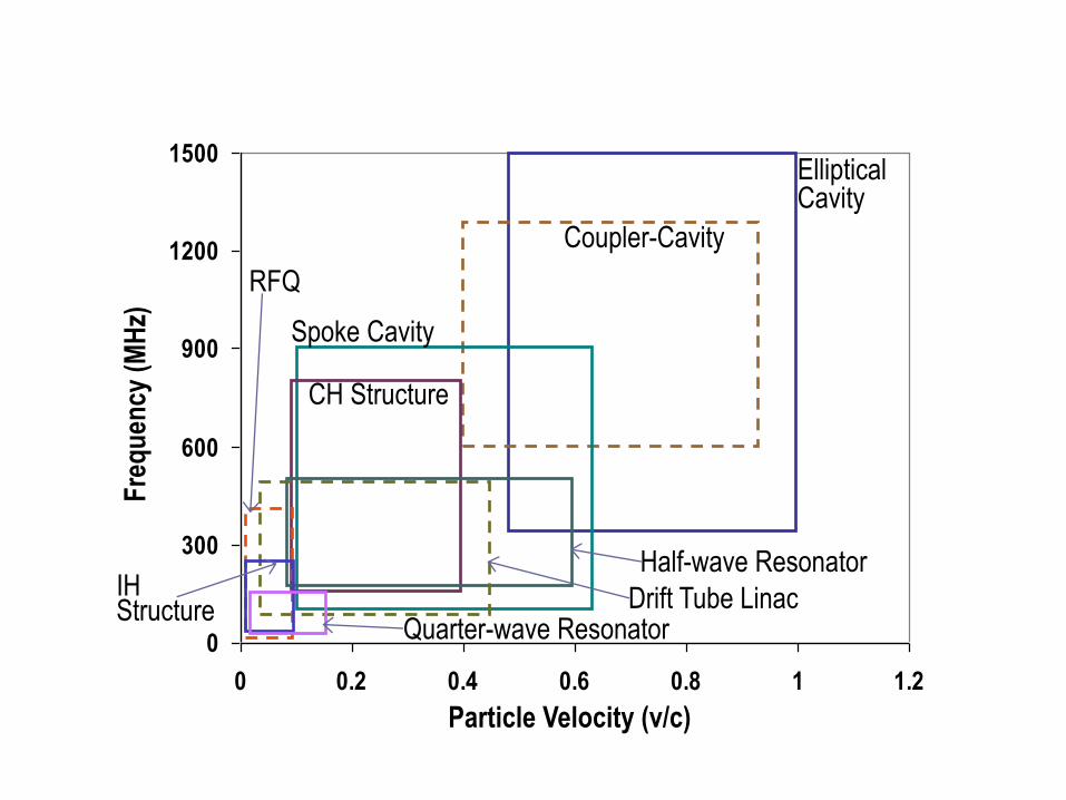
0

300

600

900

1200

1500

0 0.2 0.4 0.6 0.8 1 1.2

Particle Velocity (v/c)

Fre

qu

ency

(M

Hz)

Elliptical Cavity

Coupler-Cavity

Spoke Cavity

Half-wave Resonator

CH Structure

Drift Tube Linac Quarter-wave Resonator

RFQ

IH Structure

Typical layout of Ion-Linac

(DTL or)

superconducting

Structures

: /4, /2, spoke

Ion Source

(chopper) RFQ

(CCL or)

High velocity SRF structure

:spoke, elliptical

• In the SNS, CCL accelerates beam up to 186 MeV and 2 beta-sections of

elliptical cavities (0.61 & 0.81) to 1 GeV (power upgrade to 1.3 GeV)

• Superconducting structures are adapted for low energy regions (=<100

MeV) in newly proposed linacs (FRIB, Project-X, ESS, …): SRF structures

are expanding their applications to lower beta regions.

50-100 keV

2-7 MeV ~100 MeV ~1 GeV

or higher Wproton =

Project-X (FNAL) design: CW, 3 GeV, 3 MW

ESS (EU, Sweden) design:

Pulsed : 2.5 GeV, 4 % beam duty, 20 Hz, 50 mA during pulse, 5 MW

2.5

DTL

86.8

CCL

402.5 MHz 805 MHz

SRF, b=0.61 SRF, b=0.81

186 387 1000 MeV

Linac; 1 GeV acceleration

PUP Liquid Hg

Target

259 m

SNS (ORNL) in operation:

1 GeV, 6 % beam duty, 60 Hz,

26 mA during pulse, 1.44 MW to target

SRF structure for low & medium beta ranges

AAA/LANL, 350 MHz, b=0.175, 2-gap spoke cavity

LANL

Prototype for ion beam acceleration

850 MHz, b=0.28, 2-gap spoke cavity

JLab

345 MHz, b=0.4,

3-gap spoke cavity

for ion beam acceleration

ANL

Comparisons of RF properties

(elliptical cavity and spoke cavity)

Ex)

3 spoke cavities (402.5 MHz), and 4 elliptical cavities (805 MHz) optimally

designed for simple RF property comparisons

for proton under the same criteria: Ep~40 MV/m, Bp~85 mT.

k=1.5 % for Elliptical cavity

0.0E+00

2.0E+00

4.0E+00

6.0E+00

8.0E+00

1.0E+01

1.2E+01

1.4E+01

1.6E+01

1.8E+01

2.0E+01

0 0.1 0.2 0.3 0.4 0.5 0.6 0.7 0.8 0.9 1

Beta

Eo

TL

(M

V)

b=0.17 2-gap Spoke (402.5 MHz)

b=0.35 3-gap Spoke (402.5 MHz)

b=0.48 4-gap Spoke (402.5 MHz)

b=0.35 5-cell Elliptical (805 MHz)

b=0.48 6-cell Elliptical (805 MHz)

b=0.61 6-cell Elliptical (805 MHz)

b=0.81 6-cell Elliptical (805 MHz)

8.6 cm 29.8 cm

58.0 cm

32.6 cm

52.5 cm

68.2 cm

90.6 cm

0.0E+00

6.0E+00

1.2E+01

1.8E+01

2.4E+01

0 0.1 0.2 0.3 0.4 0.5 0.6 0.7 0.8 0.9 1

Beta

Eo

T (

MV

/m)

b=0.17 2-gap Spoke (402.5 MHz) b=0.35 3-gap Spoke (402.5 MHz)

b=0.48 4-gap Spoke (402.5 MHz) b=0.35 5-cell Elliptical (805 MHz)

b=0.48 6-cell Elliptical (805 MHz) b=0.61 6-cell Elliptical (805 MHz)

b=0.81 6-cell Elliptical (805 MHz)

EoT & Normalized shunt impedance

0.0E+00

2.0E+04

4.0E+04

6.0E+04

8.0E+04

1.0E+05

1.2E+05

1.4E+05

0 0.1 0.2 0.3 0.4 0.5 0.6 0.7 0.8 0.9 1

Beta

No

rma

liz

ed

sh

un

t im

pe

da

nc

e/L

,

r*R

s (

Oh

m^

2/m

)

b=0.17 2-gap Spoke (402.5 MHz) b=0.35 3-gap Spoke (402.5 MHz)b=0.48 4-gap Spoke (402.5 MHz) b=0.35 5-cell Elliptical (805 MHz)b=0.48 6-cell Elliptical (805 MHz) b=0.61 6-cell Elliptical (805 MHz)b=0.81 6-cell Elliptical (805 MHz)

General scaling references cavity parameters

Most of points in this plot: design, R&D, or prototypes

So far the SNS is the only one for proton beam in operation.

Ex. SNS SCL history and initial design concern

• Goal: 1GeV, pulsed, >1MW proton machine for spallation neutron source

• SNS baseline change from NC to SC in 2000, relatively late in the project

• RF frequency; followed that of the NC CCL (from LANSCE)

• Two beta groups: 0.61 and 0.81 after CCL module 4 (186 MeV)

- Cost, schedules for prototyping

• Beam dynamics with doublet lattice

• 3 cavities/ medium beta cryomodule

• 4 cavities/high beta cryomodule

• SRF Cavity designs were mainly driven by two constraints

– Power coupler; maximum 350 kW (later increased to >550 kW)

– Cavity peak surface field; 27.5 MV/m field emission concerns

• Constant gradient/cavity

• Later increase to 35 MV/m for HB cavities by adapting EP

• With one FPC to cavity; HB cavity 6 cell

• Long. Phase slip at low energy; MB cavity 6 cell

• Power coupler; scaled from KEK 508 MHz coupler

• HOM coupler; scaled from TTF HOM coupler

• Mechanical tuner; adapted from Saclay-TTF design for TESLA cavities

• Piezo tuner; incorporated into the dead leg for possible big LFD (later on)

• Cryomodule; similar construction arrangement employed in CEBAF

• Nb material RRR>250 for cells and Reactor grade Nb for Cavity end- group

• And then usual optimization process

– TTF, peak surface field balancing, raise the resonant mechanical frequency,

LFD, HOM, etc

Ex. SNS SCL history and initial design concern (continued..)

Ex.) some selected examples during SNS SCL layout design

Final beam energy vs. betas

If Ea=30 MV/m for high betas

If Ea=25 MV/m for high betas

Finally SNS Cavities and Cryomodules look;

Fundamental

Power

Coupler

HOM

Coupler

HOM

Coupler

Field

Probe

b=0.61 Specifications:

Ea=10.1 MV/m, Qo> 5E9 at 2.1 K

Medium beta (b=0.61) cavity High beta (b=0.81) cavity

Slow

Tuner

Helium

Vessel

Fast

Tuner

b=0.81 Specifications:

Ea=15.8 MV/m, Qo> 5E9 at 2.1 K

11 CMs 12 CMs

Typical RF Gain curves of klystrons:

21b

0

50

100

150

200

250

300

350

400

450

0.0E+00 2.0E+08 4.0E+08 6.0E+08 8.0E+08 1.0E+09 1.2E+09

FCM output 2̂ (AU)

HP

M r

eadin

g,

Cav F

wd P

ow

er

(kW

)

FCM digital output amp on FCM board solid state amp (transmitter) klystron

Cavity forward power

21b

0

100

200

300

400

500

600

0.0E+00 2.0E+08 4.0E+08 6.0E+08 8.0E+08 1.0E+09 1.2E+09

FCM output^2

Kly

str

on

fo

rward

po

wer

HP

M r

ead

ing

(kW

)

KlyF 71kV

KlyF 73kV

KlyF 75kV

RF in

RF

ou

t

Stable

(about 80 % of power at saturation)

Control is unstable Control margin

FCM software driving

RF Margin:

High current in pulsed operation needs more control margin.

Optimization: Cryogenics side

Given the design of the cryogenic plant, the highest overall efficiency is not

necessarily achieved when the nominally optimal thermodynamic conditions are

reached.

Since the cryogenic plant has to run at a fixed load no matter what the actual static

and dynamic loads from the cryomodules, a more efficient use of the plant would

be at temperatures different from the designed ones.

In a large scale machine, optimization could save operating cost and capital cost

as well.

A precise optimization is quite difficult, since some parameters are unknown. But it

is always useful to understand what can affect the operating conditions.

We will use a simplified model using the SNS cavity parameters, but we will learn

the about sources/consequences and general scaling.

For the scaling we will use the estimation from

M.A. Green, et. al, Advances in Cryogenic Engineering, Vol. 37, Feb. 1992

ratio=0.035 Ln(Pcold) tanh(T/3)

/ideal= ratio opambient

op

idealTT

Tη

cold

RT

P

P

η

1

Remind the relations and equations before..

At a given cavity structure, variables are;

RBCS (T)+Rres

Additional load:

field emission, beam loss, thermal radiation from coupler with RF. etc

Duty

Static loss

Other Rs terms + coupler dynamic load + beam loss

Static load

Thermal load without RF and/or beam

Cryomodule with single intermediate thermal boundary at 50-70 K typically

1-5 W/m to the primary line (2K or 4K) depending on design and module layout

Some cryomodules for 2K operation has double intermediate thermal

boundaries at 4K and 50-70 K <0.3 W/m to the primary (2K) line

ex. very large scale, low duty machine

It is more important for large scale machines at low duty factor.

Thermal load from electron activities

Field emission is especially important.

There are pretty efficient accelerations for electrons in higher beta structures.

Electrons take energy from RF and hit the surfaces in the cryomodule, which

will generate radiation (x-ray) and will be thermal deposition on surfaces.

n 15~1 ;R

R)T

17.67exp(

T1.5

(GHz)f102RRR

res

res2

24

resBCSS

Recall equation in section 2, which is good for T<5 K for niobium.

Example: using SNS cavity parameters, we will do some parametric

analysis. (cryo_estimation.xlsx)

DTL, CCL, etc:

Long multi-cell structure.

Structures are designed for a reference velocity profile.

Final energy is determined by the design.

Field should be large enough for synchronism.

SRF cavity:

A cavity is composed of a relatively small number of cells

Structures have a large velocity acceptance.

Structures are powered independently.

Phase and field (energy gain and reference phase) are flexible.

Final energy is flexible too up to the field level at which structures can sustain

fields reliably.

Phase and Energy

Phases in elliptical cavity

Each cell amplitude and phase information are used for input values in some

beam dynamic codes.

LE

dztE(z)sinωtan-dztE(z)cosωT

0

be

bs

be

bs

s

be

0

0

bsdztE(z)sinωdztE(z)sinω

One can set an origin arbitrary.

If an origin satisfies, Electrical center of the gap:

When the field is symmetry like in examples of the previous pillbox, inner

cell, geometrical and electrical centers coincide. So the electrical center

position is not a function of particle beta.

Recall the transit time factor definition in SUPERFISH manual or text books

0

0.2

0.4

0.6

0.8

1

1.2

1.4

1.6

1.8

0.4 0.5 0.6 0.7 0.8 0.9

ele

ctri

cal c

en

ter

fro

m t

he

ge

om

etri

cal o

rigi

n (

cm)

Partical beta

Ex.) SUPERFISH FILE

61BE1_2.AM

61BE1_2.SEG

0.0E+00

2.0E+05

4.0E+05

6.0E+05

8.0E+05

1.0E+06

1.2E+06

1.4E+06

1.6E+06

-10 -5 0 5 10 15 20 25 30

Axi

al F

ield

(ar

b. s

cale

)

Axial Position (cm)

Geometrical origin

bg/2

-8

-6

-4

-2

0

2

4

6

8

10

0.4 0.5 0.6 0.7 0.8 0.9

ele

ctri

cal c

en

ter

fro

m t

he

ge

om

etri

cal o

rigi

n (

cm)

Partical beta

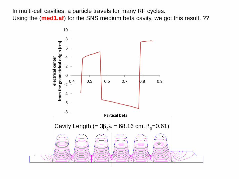
In multi-cell cavities, a particle travels for many RF cycles.

Using the (med1.af) for the SNS medium beta cavity, we got this result. ??

Cavity Length (= 3bg = 68.16 cm, bg=0.61)

-8

-6

-4

-2

0

2

4

6

8

10

0.4 0.5 0.6 0.7 0.8 0.9

ele

ctri

cal c

en

ter

fro

m t

he

ge

om

etri

cal o

rigi

n (

cm)

Partical beta

1 Both lines 1,2 satisfy the condition

be

0

0

bsdztE(z)sinωdztE(z)sinω

One corresponds max. acceleration.

The other corresponds max. deceleration.

Which one is which? 2

0

200

400

600

800

1000

1200

1400

1600

1800

2000

-50 0 50

Ph

ase

of R

F (d

eg

ree

)

axial position (cm), '0'=geometrical center

-50

-40

-30

-20

-10

0

10

20

30

40

50

-50 -30 -10 10 30 50

Ex.) 180-MeV particle enters the cavity boundary when RF phase is ‘0’

C

S

Let’s check with;

SCLE

1

LE

dztE(z)sinωdztE(z)cosωT

00

be

bs

be

bs ii

Max. accl.

Max. decel.

If a particle enters at -, maximum acceleration.

So +2n (n=integer), satisfies 2 conditions electric centers

-80

-60

-40

-20

0

20

40

60

80

100

0 100 200 300 400 500

1st cell

2nd cell

3rd cell 4th cell

5th cell

6th cell

b

Ph

ase a

t th

e e

lectr

ical cente

r (d

egre

e)

Line 1 in previous page maximum deceleration

Line 2 maximum acceleration. This should be the reference for phases of each cell.

For reference phase=0

Ex.) We can develop a spread sheet using what we exercised about Energy gain,

RF needed, Qex variations, detuning, etc. (energy_rf_power_linac.xls)

0

200

400

600

800

1000

1200

1 21 41 61 81

Beam

En

erg

y (

MeV

)

Cavity Number

0.0E+00

1.0E+05

2.0E+05

3.0E+05

4.0E+05

5.0E+05

6.0E+05

1 21 41 61 81

Po

we

r (W

)

cavity number

P_Qref

P_Q-20%

P_Q+20%

Pb

0.0E+00

5.0E+05

1.0E+06

1.5E+06

2.0E+06

2.5E+06

1 21 41 61 81

Qb

Cavity Number

0

2

4

6

8

10

12

14

16

1 21 41 61 81

En

erg

y g

ain

pe

r c

avit

y (

Me

V)

Cavity Number

0

0.1

0.2

0.3

0.4

0.5

0.6

0.7

0.8

1 21 41 61 81

Avera

ge T

ran

sit

Tim

e F

acto

r

Cavity Number

0

100

200

300

400

500

600

1 21 41 61 81

Ave

rag

e r

/Q

Cavity Number

0

20

40

60

80

100

120

140

160

1 21 41 61 81

Op

tim

um

de

tun

ing

(H

z)

Cavity Number