Chapter 7 Chapter Inferences Based on a Single Sample ... Based on a Single Sample Estimation with Confidence ... the descriptive statistics are: ... on a Single Sample Estimation

182 Chapter 7

Copyright © 2013 Pearson Education, Inc.

Inferences Based on a Single Sample Estimation with Confidence Intervals 7.2 The confidence coefficient in a confidence interval is the probability that an interval estimator

encloses the population parameter. For a 90% confidence interval, the probability that an interval will enclose the population parameter is .90. In other words, if one took repeated samples and formed 90% confidence intervals for µ, 90% of the intervals will contain µ and 10% will not.

7.4 If we were to repeatedly draw samples of size n from the population and form the interval 1.96 xx σ± each time, approximately 95% of the intervals would contain µ . We have no way

of knowing whether our interval estimate is one of the 95% that contain µ or one of the 5% that do not.

7.6 The conditions necessary to form a valid large-sample confidence interval for µ are:

1. A random sample is selected from a target population. 2. The sample size n is large, i.e., n ≥ 30

7.8 a. /2 1.96zα = , using Table IV, Appendix A, P(0 ≤ z ≤ 1.96) = .4750. Thus, / 2 .5000 .4750 .025α = − = , 2(.025) .05α = = , and1 1 .05 .95α− = − = . The

confidence level is 100% × .95 = 95%. b. /2 1.645zα = , using Table IV, Appendix A, P(0 ≤ z ≤ 1.645) = .45. Thus, / 2 .50 .45 .05α = − = , 2(.05) .10α = = , and1 1 .10 .90α− = − = . The confidence level

is 100% × .90 = 90%. c. /2 2.575zα = , using Table IV, Appendix A, P(0 ≤ z ≤ 2.575) = .495. Thus, / 2 .500 .495 .005α = − = , 2(.005) .01α = = , and1 1 .01 .99α− = − = . The confidence

level is 100% × .99 = 99%. d. /2 1.28zα = , using Table IV, Appendix A, P(0 ≤ z ≤ 1.28) = .4. Thus, / 2 .50 .40 .10α = − = , 2(.10) .20α = = , and1 1 .20 .80α− = − = . The confidence level

is 100% × .80 = 80%. e. /2 .99zα = , using Table IV, Appendix A, P(0 ≤ z ≤ .99) = .3389. Thus, / 2 .5000 .3389 .1611α = − = , 2(.1611) .3222α = = , and1 1 .3222 .6778α− = − = . The

confidence level is 100% × .6778 = 67.78%. 7.10 a. For confidence coefficient .95, .05α = and / 2 .05 / 2 .025α = = . From Table IV,

Appendix A, z.025 = 1.96. The confidence interval is:

.025

2.725.9 1.96 25.9 .56 (25.34, 26.46)

90

sx z

n± ⇒ ± ⇒ ± ⇒

Chapter

7

Inferences Based on a Single Sample Estimation with Confidence Intervals 183


b. For confidence coefficient .90, .10α = and / 2 .10 / 2 .05α = = . From Table IV, Appendix A, z.05 = 1.645. The confidence interval is:

.05

2.725.9 1.645 25.9 .47 (25.43, 26.37)

90

sx z

n± ⇒ ± ⇒ ± ⇒

c. For confidence coefficient .99, .01α = and / 2 .01 / 2 .005α = = . From Table IV,


.005

2.725.9 2.58 25.9 .73 (25.17, 26.63)

90

sx z

n± ⇒ ± ⇒ ± ⇒

7.12 a. For confidence coefficient .95, .05α = and / 2 .05 / 2 .025α = = . From Table IV,


.025

3.333.9 1.96 33.9 .647 (33.253, 34.547)

100

sx z

n± ⇒ ± ⇒ ± ⇒

b. .025

3.333.9 1.96 33.9 .323 (33.577, 34.223)

400

sx z

n± ⇒ ± ⇒ ± ⇒

c. For part a, the width of the interval is 2(.647) = 1.294. For part b, the width of the

interval is 2(.323) = .646. When the sample size is quadrupled, the width of the confidence interval is halved.

7.14 a. From the printout, the 90% confidence interval is (93.53, 109.71). We are 90%

confident that the true mean fasting blood sugar level in hypertensive patients is between 93.53 and 109.71.

b. From the printout, the 90% confidence interval is (1.92771, 1.95429). We are 90%

confident that the true mean magnesium level in hypertensive patients is between 1.92771 and 1.95429.

c. If the confidence level is raised to 95%, the width of the interval will increase. With

more confidence, we must include more number. d. If the sample size is increased from 50 to 100, the width of the interval should decrease.

The standard deviation of x will be 100

s instead of

50

s.

7.16 a. The target parameter is µ = average amount of time (in minutes) per day laptops are

used for taking notes for all middle school students across the country.

b. The standard deviation of the sampling distribution of x is estimated with s

n, not

just s. c. For confidence coefficient .90, .10α = and / 2 .05α = . From Table IV, Appendix A,

z.05 = 1.645. The confidence interval is:

184 Chapter 7


.05

19.513.2 1.645 13.2 3.116 (10.084, 16.316)

106

sx z

n± ⇒ ± ⇒ ± ⇒

We are 90% confident that the true average amount of time per day laptops are used for

taking notes for all middle school students across the country is between 10.084 and 16.316 minutes.

d. “90% confidence” means that in repeated sampling, 90% of all confidence intervals

constructed in this manner will contain the true mean. e. No, this is not a problem. The Central Limit Theorem says that the sampling

distribution of x will be approximately normal, regardless of the shape of the population being sampled from, as long as the sample size is relatively large. The sample size for this distribution is 106, which is sufficiently large.

7.18 a. The target parameter is the mean egg length for all New Zealand birds, µ . b. Using MINITAB, 50 uniform random numbers were generated between 1 and 132. Those random numbers were: 3, 9, 12, 13, 14, 15, 17, 22, 23, 24, 25, 26, 27, 29, 37, 39, 45, 49, 50, 51, 52, 54, 60, 65, 68, 70, 71, 75, 93, 95, 96, 97, 98, 99, 101, 105, 108, 109, 110, 112, 118, 119, 120, 123, 126, 127, 128, 129, 130, 131 The egg lengths corresponding to these numbers were then selected. The 50 egg lengths are:

57, 44, 31, 36, 61, 67, 69, 48, 58, 61, 59, 65, 66, 46, 56, 64, 49, 40, 58, 30, 28, 43, 45, 42, 52, 40, 46, 74, 26, 23, 23, 19.5, 20, 23.5, 17, 19, 40, 35, 29, 45, 110, 124, 160, 205, 192, 125, 195, 218, 236, 94

c. Using MINITAB, the descriptive statistics are:

Descriptive Statistics: Egg Length Variable N Mean StDev Minimum Q1 Median Q3 Maximum Egg Length 50 8.28 55.65 17.00 34.00 48.50 67.50 236.00

The mean is x = 68.28 and the standard deviation is s = 55.65.

d. For confidence coefficient .99, .01α = and / 2 .01 / 2 .005α = = . From Table IV, Appendix A, z.005 = 2.58. The 99% confidence interval is:

.005

55.652.58 68.28 2.58 68.28 20.30 (47.98, 88.58)

50x z x

x n

σσ± ⇒ ± ⇒ ± ⇒ ± ⇒

e. We are 99% confident that the mean egg length of the bird species of New Zealand is

between 47.98 and 88.58 mm.



7.20 a. The parameter of interest is µ = the true mean shell length of all green sea turtles in the lagoon.

b. Using MINITAB, the descriptive statistics are: Descriptive Statistics: Length Variable N Mean StDev Minimum Q1 Median Q3 Maximum Length 76 55.47 11.34 30.37 49.20 56.79 64.70 81.63 The point estimate of µ is 55.47x = . c. For confidence coefficient .95, .05α = and / 2 .025α = . From Table IV, Appendix A,

z.025 = 1.96. The confidence interval is:

.025

11.3455.47 1.96 55.47 2.55 (52.92, 58.02)

76

sx z

n± ⇒ ± ⇒ ± ⇒

We are 95% confident that the true mean shell length of all green sea turtles in the

lagoon is between 52.92 and 58.02 centimeters. d. Since 60 is not in the 95% confidence interval, it is not a likely value for the true mean.

Thus, we would be very suspicious of the claim. 7.22 a. Using MINITAB, the descriptive statistics are: Descriptive Statistics: Times

Variable N Mean StDev Minimum Q1 Median Q3 Maximum Times 38 0.1879 0.1814 -0.0100 0.0500 0.1400 0.3000 0.9000

For confidence coefficient .95, .05α = and / 2 .025α = . From Table IV, Appendix A, z.025 = 1.96. The confidence interval is:

.025

.1814.1879 1.96 .1879 .0577 (.1302, .2456)

38

sx z

n± ⇒ ± ⇒ ± ⇒

We are 95% confident that the true mean decrease in sprint times for the population of

all football players who participate in the speed training program is between .1302 and .2456 seconds.

b. Yes, the training program really is effective. If the training program was not effective,

then the mean decrease in sprint times would be 0. We note that 0 is not in the 95% confidence interval. Therefore, it is not a likely value for the true mean.

7.24 Using MINITAB, the descriptive statistics are: Descriptive Statistics: ATTIMES Variable N Mean StDev Minimum Q1 Median Q3 Maximum ATTIMES 50 20.85 13.41 0.800 10.35 19.65 30.18 48.20

186 Chapter 7


For confidence coefficient .90, .10α = and / 2 .10 / 2 .05α = = . From Table IV, Appendix A, z.05 = 1.645. The 90% confidence interval is:

.05

13.411.645 20.85 1.645 20.85 3.12 (17.73, 23.97)

50xx z x

n

σσ± ⇒ ± ⇒ ± ⇒ ± ⇒

We are 90% confident that the mean attention time given to all twin boys by their parents is between 17.73 and 23.97 hours.

7.26 11,298

2.265,000

x = =

For confidence coefficient, .95, .05α = and / 2 .05 / 2 .025α = = . From Table IV, Appendix A, z.025 = 1.96. The confidence interval is:

/2

1.52.26 1.96 2.26 .04 (2.22, 2.30)

5000

sx z

nα± ⇒ ± ⇒ ± ⇒

We are 95% confident the mean number of roaches produced per roach per week is between

2.22 and 2.30. 7.28 Both the z-distribution and the t-distribution are mound-shaped and symmetric with mean 0.

The primary difference between the z- and t-distributions is that the t-distribution is more spread out than the z-distribution.

7.30 a. For confidence coefficient .80, 1 .80 .20α = − = and / 2 .20 / 2 .10α = = . From Table IV,

Appendix A, z.10 = 1.28. From Table VI, with df = n − 1 = 7 − 1 = 6, t.10 = 1.440. b. For confidence coefficient .90, 1 .90 .10α = − = and / 2 .10 / 2 .05α = = . From Table IV,

Appendix A, z.05 = 1.645. From Table VI, with df = n − 1 = 7 − 1 = 6, t.05 = 1.943. c. For confidence coefficient .95, 1 .95 .05α = − = and / 2 .05 / 2 .025α = = . From Table

IV, Appendix A, z.025 = 1.96. From Table VI, with df = n − 1 = 7 − 1 = 6, t.025 = 2.447. d. For confidence coefficient .98, 1 .98 .02α = − = and / 2 .02 / 2 .01α = = . From Table IV,

Appendix A, z.01 = 2.33. From Table VI, with df = n − 1 = 7 − 1 = 6, t.01 = 3.143. e. For confidence coefficient .99, 1 .99 .01α = − = and / 2 .01 / 2 .005α = = . From Table

IV, Appendix A, z.005 = 2.58. From Table VI, with df = n − 1 = 7− 1 = 6, t.005 = 3.707. f. Both the t and z-distributions are symmetric

around 0 and mound-shaped. The t-distribution is more spread out than the z-distribution.



7.32 a. P(−t0 < t < t0) = .95 where df = 16 Because of symmetry, the statement can be written P(0 < t < t0) = .475 where df = 16 ⇒ P(t ≥ t0) = .5 − .475 = .025 t0 = 2.120 b. P(t ≤ −t0 or t ≥ t0) = .05 where df = 16 ⇒ 2P(t ≥ t0) = .05 ⇒ P(t ≥ t0) = .025 where df = 16 t0 = 2.120 c. P(t ≤ t0) = .05 where df = 16 Because of symmetry, the statement can be written P(t ≥ −t0) = .05 where df = 16 t0 = −1.746 d. P(t ≤ −t0 or t ≥ t0) = .10 where df = 12 ⇒ 2P(t ≥ t0) = .10 ⇒ P(t ≥ t0) = .05 where df = 12 t0 = 1.782 e. P(t ≤ −t0 or t ≥ t0) = .01 where df = 8 ⇒ 2P(t ≥ t0) = .01 ⇒ P(t ≥ t0) = .005 where df = 8 t0 = 3.355 7.34 For this sample,

1567

97.937516

xx

n= = =∑

( )22

2

2

1567155,867

16 159.92921 16 1

xx

nsn

− −= = =

− −

∑∑

2 12.6463s s= = a. For confidence coefficient, .80, 1 .80 .20α = − = and / 2 .20 / 2 .10α = = . From Table

VI, Appendix A, with df = n − 1 = 16 − 1 = 15, t.10 = 1.341. The 80% confidence interval for µ is:

.10

12.646397.94 1.341 97.94 4.240 (93.700, 102.180)

16

sx t

n± ⇒ ± ⇒ ± ⇒

188 Chapter 7


b. For confidence coefficient, .95, 1 .95 .05α = − = and / 2 .05 / 2 .025α = = . From Table VI, Appendix A, with df = n − 1 = 24 − 1 = 23, t.025 = 2.131. The 95% confidence interval for µ is:

.250

12.646397.94 2.131 97.94 6.737 (91.203, 104.677)

16

sx t

n± ⇒ ± ⇒ ± ⇒

The 95% confidence interval for µ is wider than the 80% confidence interval for µ

found in part a. c. For part a: We are 80% confident that the true population mean lies in the interval 93.700 to

102.180. For part b: We are 95% confident that the true population mean lies in the interval 91.203 to

104.677. The 95% confidence interval is wider than the 80% confidence interval because the

more confident you want to be that µ lies in an interval, the wider the range of possible values.

7.36 a. For confidence coefficient .99, .01α = and / 2 .005α = . From Table VI, Appendix A,

with df = n – 1 = 6 – 1 = 5, t.005 = 4.032. The confidence interval is:

.005,5

6.852.9 4.032 52.9 11.91 (41.71, 64.09)

6

sx t

n± ⇒ ± ⇒ ± ⇒

We are 99% confident that the true mean shell length of all green sea turtles in the

lagoon is between 41.71 and 64.09 cm.



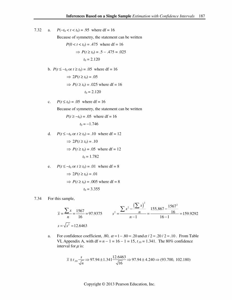
b. We must assume that the data are sampled from a normal distribution and that the sample was randomly selected. A histogram of the data is:

Length

Freq

uenc

y

807060504030

14

12

10

8

6

4

2

0

Mean 55.47StDev 11.34N 76

Histogram of LengthNormal

These data do not look that normal. The confidence interval may not be valid. 7.38 For confidence coefficient .90, .10α = and / 2 .10 / 2 .05α = = . From Table VI, Appendix A, with df = n – 1 = 25 – 1 = 24, t.05 = 1.711. The 90% confidence interval is:

.05,24

10.975.4 1.711 75.4 3.73 (71.67, 79 13)

25

sx t .

n± ⇒ ± ⇒ ± ⇒

We are 90% confident that the true mean breaking strength of white wood is between 71.67 and 79.13 MPa’s. 7.40 a. The point estimate for the average annual rainfall amount at ant sites in the Dry Steppe region of Central Asia is x =183.4 milliliters.

b. For confidence coefficient .90, .10α = and / 2 .10 / 2 .05α = = . From Table VI, Appendix A, with df = n – 1 = 5 – 1 = 4, t.05 = 2.132.

c. The 90% confidence interval is:

.05

20.6470183.4 2.132 183.4 19.686 (163.714, 203.086)

5

sx t

n± ⇒ ± ⇒ ± ⇒

d. We are 90% confident that the average annual rainfall amount at ant sites in the Dry

Steppe region of Central Asia is between 163.714 and 203.086 milliliters.

e. Using MINITAB, the 90% confidence interval is: One-Sample T: DS Rain Variable N Mean StDev SE Mean 90% CI DS Rain 5 183.400 20.647 9.234 (163.715, 203.085)

190 Chapter 7


The 90% confidence interval is (163.715, 203.085). This is very similar to the confidence interval calculated in part c.

f. The point estimate for the average annual rainfall amount at ant sites in the Gobi Desert region of Central Asia is x =110.0 milliliters.

For confidence coefficient .90, .10α = and / 2 .10 / 2 .05α = = . From Table VI, Appendix A, with df = n – 1 = 6 – 1 = 5, t.05 = 2.015.

The 90% confidence interval is:

.05

15.975110.0 2.015 110.0 13.141 (96.859, 123.141)

6

sx t

n± ⇒ ± ⇒ ± ⇒

We are 90% confident that the average annual rainfall amount at ant sites in the Gobi Desert region of Central Asia is between 96.859 and 123.141 milliliters.

Using MINITAB, the 90% confidence interval is:

One-Sample T: GD Rain Variable N Mean StDev SE Mean 90% CI GD Rain 6 110.000 15.975 6.522 (96.858, 123.142)

The 90% confidence interval is (96.858, 123.142). This is very similar to the confidence interval calculated above.

7.42 Some preliminary calculations are:

247

1913

xx

n= = =∑

( )22

2

2

2474751

5813 4.83331 13 1 12

xx

nsn

− −= = = =

− −

∑∑

4.8333 2.198s = = For confidence coefficient .99, .01α = and / 2 .01 / 2 .005α = = . From Table VI, Appendix

A, with df = n – 1 = 13 – 1 = 12, t.005 = 3.055. The 99% confidence interval is:

.005,12

2.19819 3.055 19 1.86 (17.14, 20.86)

13

sx t

n± ⇒ ± ⇒ ± ⇒

We are 99% confident that the true mean quality of all studies on the treatment of

Alzheimer’s disease is between 17.14 and 20.86.



7.44 a. Some preliminary calculations are:

7,169

358.4520

xx

n= = =∑

( )22

2

2

7,1692,833, 465

263,736.9520 13,880.892111 20 1 19

xx

nsn

− −= = = =

− −

∑∑

13,880.89211 117.8172s = = For confidence coefficient .95, .05α = and / 2 .05 / 2 .025α = = . From Table VI,

Appendix A, with df = n – 1 = 20 – 1 = 19, t.025 = 2.093. The 95% confidence interval is:

.025

117.8172358.45 2.093 358.45 55.140 (303.310, 413.590)

20

sx t

n± ⇒ ± ⇒ ± ⇒

b. We are 95% confident that the true mean skidding distance for the road is between

303.310 and 413.590 meters.

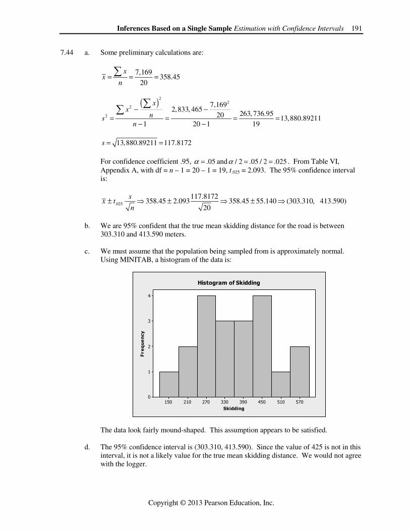
c. We must assume that the population being sampled from is approximately normal. Using MINITAB, a histogram of the data is:

Skidding

Fre

qu

en

cy

570510450390330270210150

4

3

2

1

0

Histogram of Skidding

The data look fairly mound-shaped. This assumption appears to be satisfied.

d. The 95% confidence interval is (303.310, 413.590). Since the value of 425 is not in this interval, it is not a likely value for the true mean skidding distance. We would not agree with the logger.

192 Chapter 7


7.46 a. Some preliminary calculations are:

196

17.8211

xx

n= = =∑

( )1636.24

11111

196734,3

1

22

2

2 =−

−=

−

−=

∑∑n

n

xx

s

92.41636.26 ==s For confidence coefficient .95, .05α = and / 2 .05 / 2 .025α = = . From Table VI, with

df = n – 1 = 11 – 1 = 10, t.025 = 2.228. The 95% confidence interval is:

x )13.21,51.14(31.382.1711

92.4228.282.172/ ⇒±⇒±⇒±

n

stα

We are 95% confident that the mean FNE score of the population of bulimic female

students is between 14.51 and 21.13. b. Some preliminary calculations are:

14.1414

198 === ∑n

xx

( )9780.27

11414

198164,3

1

22

2

2 =−

−=

−

−=

∑∑n

n

xx

s

29.59780.27 ==s For confidence coefficient .95, .05α = and / 2 .05 / 2 .025α = = . From Table VI, with

df = n – 1 = 14 – 1 = 13, t.025 = 2.160. The 95% confidence interval is:

)19.17,09.11(05.314.1414

29.5160.214.142/ ⇒±⇒±⇒±

n

stx α

We are 95% confident that the mean FNE score of the population of normal female

students is between 11.09 and 17.19. c. We must assume that the populations of FNE scores for both the bulimic and normal

female students are normally distributed.



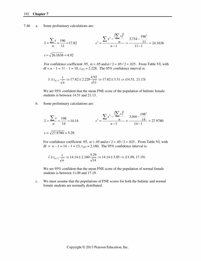
Stem-and-leaf displays for the two groups are below: Stem-and-leaf of Bulimia N = 11 Leaf Unit = 1.0 1 1 0 3 1 33 4 1 4 5 1 6 (1) 1 9 5 2 011 2 2 2 2 45 Stem-and-leaf of Normal N = 14 Leaf Unit = 1.0 2 0 67 3 0 8 5 1 01 7 1 33 7 1 5 6 1 6 5 1 899 2 2 0 1 2 3

From both of these plots, the assumption of normality is questionable for both groups.

Neither of the plots looks mound-shaped. However, it is hard to decide with such small sample sizes.

7.48 By the Central Limit Theorem, the sampling distribution of p̂ is approximately normal with

mean p̂ pµ = and standard deviationn

pqp =ˆσ .

7.50 If p is near 0 or 1, an extremely large sample size is required. For example if p = .01, then

15np ≥ implies that 15 15

1500..01

np

≥ = =

7.52 a. The sample size is large enough if both ˆ 15np ≥ and ˆ 15nq ≥ . ˆ 144(.76) 109.44np = = and ˆ 144(.24) 34.56nq = = . Since both of these numbers are

greater than or equal to 15, the sample size is sufficiently large to conclude the normal approximation is reasonable.

b. For confidence coefficient .90, .10α = and / 2 .10 / 2 .05α = = . From Table IV,

Appendix A, z.05 = 1.645. The 90% confidence interval is:

.05

ˆ ˆ .76(.24)ˆ ˆ 1.645 .76 1.645 .76 .059 (.701, .819)

144

pq pqp z p

n n± ≈ ± ⇒ ± ⇒ ± ⇒

194 Chapter 7


c. We must assume the sample was randomly selected from the population of interest. We must also assume our sample size is sufficiently large to ensure the sampling distribution is approximately normal. From the results of part a, this appears to be a reasonable assumption.

7.54 a. Of the 50 observations, 15 like the product15

ˆ .3050

p⇒ = = .

The sample size is large enough if both ˆ 15np ≥ and ˆ 15nq ≥ . ˆ 50(.3) 15np = = and ˆ 50(.7) 35nq = = . Since both of these numbers are greater than or equal to 15, the sample size is sufficiently large to conclude the normal approximation is reasonable. For the confidence coefficient .80, .20α = and / 2 .20 / 2 .10α = = . From Table IV,


.10

ˆ ˆ .3(.7)ˆ .3 1.28 .3 .083 (.217, .383)

50

pqp z

n± ⇒ ± ⇒ ± ⇒

b. We are 80% confident the proportion of all consumers who like the new snack food is

between .217 and .383. 7.56 a. The estimate of the true proportion of satellite radio subscribers who have a satellite

radio receiver in their car is396

ˆ .79.501

p = =

b. The sample size is large enough if both ˆ 15np ≥ and ˆ 15nq ≥ . For this problem, ˆ .79.p =

ˆ 501(.79) 395.79np = = and ˆ 501(.21) 105.21nq = = . Since both of these numbers are greater than or equal to 15, the sample size is sufficiently large to conclude the normal approximation is reasonable.

For confidence coefficient .90, .10α = and / 2 .10 / 2 .05α = = . From Table IV,


.05

ˆ ˆ .79(.21)ˆ ˆ 1.645 .79 1.645 .79 .030 (.760, .820)

501

pq pqp z p

n n± ≈ ± ⇒ ± ⇒ ± ⇒

c. We are 90% confident that the true proportion of all of satellite radio subscribers who

have a satellite radio receiver in their car is between .760 and .820. 7.58 a. The parameter of interest is the true proportion of fillets that are really red snapper.



b. The sample size is large enough if both ˆ 15np ≥ and ˆ 15nq ≥ . ˆ 22(.23) 5.06np = = and ˆ 22(.77) 16.94nq = = . Since the first number is not greater than

or equal to 15, the sample size is not sufficiently large to conclude the normal approximation is reasonable.

c. The Wilson adjusted sample proportion is

2 5 2 7

.2694 22 4 26

xp

n

+ += = = =+ +


Appendix A, z.025 = 1.96. The Wilson adjusted 95% confidence interval is:

.025

(1 ) .269(.731).269 1.96 .269 .170 (.099, .439)

4 22 4

p pp z

n

−± ⇒ ± ⇒ ± ⇒+ +

d. We are 95% confident that the true proportion of fish fillets purchased from vendors

across the U.S. that are really red snapper is between .099 and .439.

7.60 a. Of the 38 times, only one was negative. Thus, 37

ˆ .974.38

p = =

b. The sample size is large enough if both ˆ 15np ≥ and ˆ 15nq ≥ . For this problem,

ˆ .974.p = ˆ 38(.974) 37.012np = = and ˆ 38(.026) 0.988.nq = = Since one of these numbers is less

than 15, the sample size may not be sufficiently large to conclude the normal approximation is reasonable.

The Wilson adjusted sample proportion is

2 37 2 39

.9294 38 4 42

xp

n

+ += = = =+ +

For confidence coefficient .95, α = .05 and α/2 = .05/2 = .025. From Table IV,

Appendix A, z.025 = 1.96. The Wilson adjusted 95% confidence interval is:

.025

(1 ) .929(.071).929 1.96 .929 .078 (.851, 1.007)

4 38 4

p pp z

n

−± ⇒ ± ⇒ ± ⇒+ +

We are 95% confident that the true proportion of “improved” sprint times is between

.851 and 1.

196 Chapter 7


7. 62 First, we compute p̂ : 88

ˆ .175504

xp

n= = =

The sample size is large enough if both 15ˆ ≥pn and 15ˆ ≥qn . 2.88)175(.504ˆ ==pn and 8.415)825(.504ˆ ==qn . Since both of the numbers are greater than

or equal to 15, the sample size is sufficiently large to conclude the normal approximation is reasonable.

For confidence coefficient .90, .10α = and / 2 .10 / 2 .05α = = . From Table IV, Appendix A,

z.05 = 1.645. The 90% confidence interval is:

)203.,147(.028.175.504

)825(.175.645.1175.

ˆˆ645.1ˆˆ 05. ⇒±⇒±⇒±⇒±

n

qpp

n

pqzp

We are 90% confident that the true proportion of all ice melt ponds in the Canadian Arctic that have first-year ice is between .147 and .203.

7.64 a. The estimate of the true proportion of all U. S. teenagers who have used at least one

informal element in a school writing assignment is 52

ˆ .021.2481

p = =

The sample size is large enough if both ˆ 15np ≥ and ˆ 15nq ≥ .

ˆ 2481(.021) 52.10np = = and ˆ 2481(.979) 2428.90nq = = . Since both of these numbers are greater than or equal to 15, the sample size is sufficiently large to conclude the normal approximation is reasonable.



.025

ˆ ˆ .021(.979)ˆ ˆ 1.96 .021 1.96 .021 .0056 (.0154, .0266)

2481

pq pqp z p

n n± ≈ ± ⇒ ± ⇒ ± ⇒

We are 95% confident that the true proportion of all people in the world who suffer from

ORS is between .0154 and .0266. b. The population of interest is all people in the world. The sample was selected from

2,481 university students in Japan. This sample is probably not representative of the population. There are several problems with this sample. First, it is made up of only Japanese people, which may not be representative of all the adults in the world. Next, the age group is very limited, probably in the range of 18 to 24. Finally, those people who attend universities may not be representative of all people. Thus, the inference made from this sample may not be valid for all of the people of the world.



7.66 The Wilson adjusted sample proportion is

2 3 2 5

.2944 13 4 17

xp

n

+ += = = =+ +

For confidence coefficient .99, .01α = and / 2 .01 / 2 .005α = = . From Table IV, Appendix A, z.005 = 2.58. The Wilson adjusted 99% confidence interval is:

.005

(1 ) .294(.706).294 2.58 .294 .285 (.009, .579)

4 13 4

p pp z

n

−± ⇒ ± ⇒ ± ⇒+ +

We are 99% confident that the true proportion of all studies on the treatment of Alzheimer’s disease with a Wong score below 18 is between .009 and .579.

7.68 The sampling error, SE, is half the width of the confidence interval. 7.70 The statement “For a fixed confidence level (1 )α− , increasing the sampling error SE will

lead to a smaller n when determining sample size” is True. 7.72 The sample size will be larger than necessary for any p other than .5. 7.74 a. For confidence coefficient .95, .05α = and / 2 .05 / 2 .025α = = . From Table IV,

Appendix A, z.025 = 1.96.

The sample size is ( )2 2

/22 2

(1.96) (.3)(.7)224.1 225

( ) .06

z pqn

SEα= = = ≈

You would need to take n = 225 samples. b. To compute the needed sample size, use:

( )2 2

/22 2

(1.96) (.5)(.5)266.8 267

( ) .06

z pqn

SEα= = = ≈

You would need to take n = 267 samples. 7.76 a. To compute the needed sample size, use

( )2 2

/22( )

zn

SEα σ

= where 1 .95 .05α = − = and / 2 .05 / 2 .025α = =

From Table IV, Appendix A, z.025 = 1.96. For a width of 4 units, SE = 4/2 = 2.

2 2

2

(1.96) (12)138.298 139

2n = = ≈

You would need to take 139 samples at a cost of 139($10) = $1390. No, you do not

have sufficient funds.

198 Chapter 7


b. For confidence coefficient .90, .10α = and / 2 .10 / 2 .05α = = . From Table IV, Appendix A, z.05 = 1.645.

2 2

2

(1.645) (12)97.417 98

2n = = ≈

You would need to take 98 samples at a cost of 98($10) = $980. You now have

sufficient funds but have an increased risk of error. 7.78 For confidence coefficient .95, .05α = and / 2 .05 / 2 .025α = = . From Table IV, Appendix

A, z.025 = 1.96. Since we have no previous knowledge about the proportion of cul-de-sac homes in home town that were burglarized in the past year, we will use .5 to estimate p.

2 2

/22 2

1.96 (.5)(.5)2401

( ) .02

z pqn

SEα= = =

We need to find out whether each home in the sample of 2,401 cul-de-sac homes was

burglarized in the last year or not. 7.80 a. The confidence level desired by the researchers is .95.

b. The sampling error desired by the researchers is SE = .001.

c. For confidence coefficient .95, .05α = and / 2 .05 / 2 .025α = = . From Table IV, Appendix A, z.025 = 1.96.

The sample size is 2 2 2 2

.0252 2

( ) 1.96 (.005)96.04 97

( ) .001

zn

SE

σ= = = ≈ .

7.82 For confidence coefficient .90, .10α = and / 2 .10 / 2 .05α = = . From Table IV, Appendix A, z.05 = 1.645. Since we have no estimate given for the value of p, we will use .5. The

confidence interval is:

2 2

/22 2

1.645 .5(.5)1,691.3 1,692

( ) .02

z pqn

SEα= = = ≈

7.84 a. From Exercise 7.37, s = 129.565. We will use this to estimate the population standard

deviation. The necessary sample size is:

2 2 2 2

/22 2

1.96 (129.656)31.89 32

( ) 45

zn

SEα σ= = = ≈



b. Answers will vary. Since we want to have the sample spread fairly evenly through out the year, we might want to randomly sample 2 days from each month. That would give us a sample size of 24. Then, we can randomly select 8 more months and randomly select a 3rd day in each of those months.

A simpler method might be to use a sample size of 36 (to be conservative) and randomly

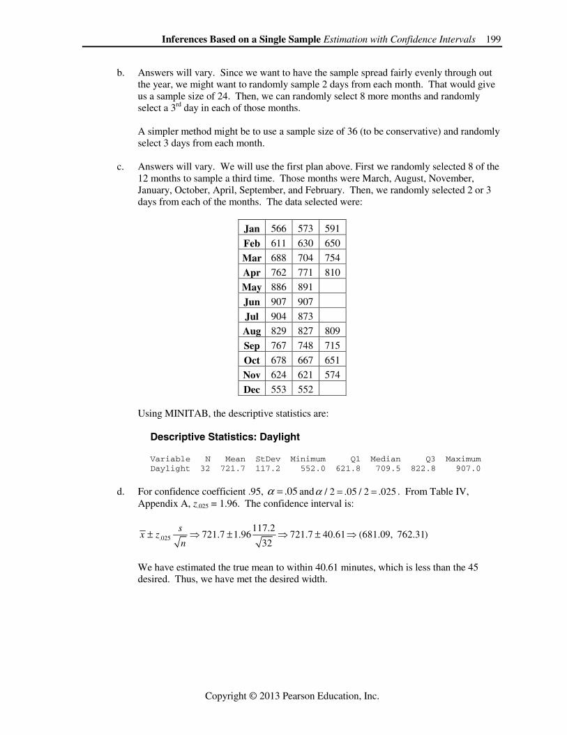
select 3 days from each month. c. Answers will vary. We will use the first plan above. First we randomly selected 8 of the

12 months to sample a third time. Those months were March, August, November, January, October, April, September, and February. Then, we randomly selected 2 or 3 days from each of the months. The data selected were:

Jan 566 573 591

Feb 611 630 650

Mar 688 704 754

Apr 762 771 810

May 886 891

Jun 907 907

Jul 904 873

Aug 829 827 809

Sep 767 748 715

Oct 678 667 651

Nov 624 621 574

Dec 553 552 Using MINITAB, the descriptive statistics are:

Descriptive Statistics: Daylight

Variable N Mean StDev Minimum Q1 Median Q3 Maximum Daylight 32 721.7 117.2 552.0 621.8 709.5 822.8 907.0

d. For confidence coefficient .95, .05α = and / 2 .05 / 2 .025α = = . From Table IV,


.025

117.2721.7 1.96 721.7 40.61 (681.09, 762.31)

32

sx z

n± ⇒ ± ⇒ ± ⇒

We have estimated the true mean to within 40.61 minutes, which is less than the 45

desired. Thus, we have met the desired width.

200 Chapter 7


7.86 From Exercise 7.60, our estimate of p is ˆ .974.p = We will use this to estimate the sample size.

For confidence coefficient .95, .05α = and / 2 .05 / 2 .025α = = . From Table IV, Appendix

A, z.025 = 1.96.

2 2

/22 2

1.96 (.974)(.026)108.09 109

( ) .03

z pqn

SEα= = = ≈

We would need to sample 109 high school athletes. 7. 88 a. The confidence interval might lead to an erroneous inference because the sample size

used is probably too small. Recall that the sample size is large enough if both ˆ 15np ≥

and ˆ 15nq ≥ . For this problem, 10

ˆ .556.18

p = = ˆ 18(.556) 10.008np = = and

ˆ 18(.444) 7.992nq = = . Neither of these two values is greater than 15. Thus, the sample size is not sufficiently large to conclude the normal approximation is reasonable.

b. For confidence coefficient .95, .05α = and / 2 .05 / 2 .025α = = . From Table IV,

Appendix A, z.025 = 1.96. From the previous study, we will use 10

ˆ .55618

p = = to

estimate p.

2 2

/22 2

1.96 (.556)(.444)592.72 593

( ) .04

z pqn

SEα= = = ≈

7.90 Range 180 60

304 4

σ −≈ = =

For confidence coefficient .95, .05α = and / 2 .05 / 2 .025α = = . From Table IV, Appendix

A, z.025 = 1.96.


/22 2

1.96 (30)138.3 139

( ) 5

zn

SEα σ= = = ≈

7.92 a. For confidence coefficient .90, .10α = and / 2 .10 / 2 .05α = = . From Table IV,

Appendix A, z.05 = 1.645.


/22 2

1.645 (2 )1082.4 1083

( ) .1

zn

SEα σ= = = ≈

b. In part a, we found n = 1083. If we used an n of only 100, the width of the confidence

interval for µ would be wider since we would be dividing by a smaller number.



c. We know /2/2

.1 100.5

2

z SE nSE z

nα

ασ

σ= ⇒ = = =

P(−.5 ≤ z ≤ .5) = .1915 + .1915 = .3830. Thus, the level of confidence is approximately

38.3%. 7.94 We must take a random sample from the target population and the distribution of the

population must be approximately normal.

7.96 a. / 2 .05 / 2 .025α = = ; 2.025,7 16.0128χ =

and

2.975,7 1.68987χ =

b. / 2 .10 / 2 .05α = = ; 2.05,16 26.2962χ = and 2

.95,16 7.96164χ =

c. / 2 .01 / 2 .005α = = ; 2.005,20 39.9968χ = and 2

.995,20 7.43386χ =

d. / 2 .05 / 2 .025α = = ; 2.025,20 34.1696χ = and 2

.975,20 9.59083χ =

7.98 To find the 90% confidence interval forσ , we need to take the square root of the end points

of the 90% confidence interval for 2σ from exercise 7.97. a. The 90% confidence interval forσ is:

4.537 8.809 2.130 2.968σ σ≤ ≤ ⇒ ≤ ≤ b. The 90% confidence interval forσ is:

.00024 .00085 .0155 .0292σ σ≤ ≤ ⇒ ≤ ≤ c. The 90% confidence interval forσ is:

641.86 1,809.09 25.335 42.533σ σ≤ ≤ ⇒ ≤ ≤ d. The 90% confidence interval forσ is:

.94859 12.6632 .97396 3.55854σ σ≤ ≤ ⇒ ≤ ≤ 7.100 a. The target parameter is the variance of the WR scores among all drug dealers. b. For confidence level .99, .01α = and / 2 .01 / 2 .005α = = . From Table VII, Appendix

A, with df = n – 1 = 100 - 1 = 99, 2.005,99 140.169χ ≈ and 2

.995,99 67.3276χ ≈ . The 99%

confidence interval is:

2 2 2 2

2 2 22 2.005 .995

( 1) ( 1) (100 1)6 (100 1)625.426 52.935

140.169 67.3276

n s n sσ σ σχ χ− − − −≤ ≤ ⇒ ≤ ≤ ⇒ ≤ ≤

202 Chapter 7


c. This means that in repeated sampling, 99% of all confidence intervals constructed in the same manner will contain the target parameter.

d. We must assume that a random sample was selected from the target population and that

the population is approximately normally distributed. e. We can use the standard deviation rather than the variance to find a reasonable range for

the value of the population mean. f. To find the 99% confidence interval forσ , we need to take the square root of the end

points of the 99% confidence interval for 2σ .

25.426 52.935 5.042 7.276σ σ≤ ≤ ⇒ ≤ ≤ We are 99% confident that the true standard deviation of the WR scores of drug dealers

is between 5.042 and 7.276. 7.102 For confidence level .90, .10α = and / 2 .10 / 2 .05α = = . From Table VII, Appendix A, with

df = n – 1 = 4-1 = 3, 2.05,3 7.81473χ = and 2

.95,3 .351846χ = . The 90% confidence interval is:

2 2 2 2

2 2 22 2.05 .95

( 1) ( 1) (4 1).13 (4 1).13.0065 .1441

7.81473 .351846

n s n sσ σ σχ χ− − − −≤ ≤ ⇒ ≤ ≤ ⇒ ≤ ≤

We are 90% confident that the true variance of the peptide scores for alleles of the antigen-

produced protein is between .0065 and .1441. 7.104 a. For confidence level .95, .05α = and / 2 .05 / 2 .025α = = . From Table VII, Appendix

A, with df = n – 1 = 18 - 1 = 17, 2.025,17 30.1910χ = and 2

.975,17 7.56418χ = . The 95%

confidence interval for the variance is:

2 2 2 2

2 2 22 2.025 .975

( 1) ( 1) (18 1)6.3 (18 1)6.322.349 89.201

30.1910 7.56418

n s n sσ σ σχ χ− − − −≤ ≤ ⇒ ≤ ≤ ⇒ ≤ ≤

The 95% confidence interval for the standard deviation is:

22.349 89.201 4.727 9.445σ σ≤ ≤ ⇒ ≤ ≤

b. We are 95% confident that the true standard deviation of the conduction times of the prototype system is between 4.727 and 9.445.

c. No. Since 7 falls in the 95% confidence interval, it is a likely value for the population

standard deviation. Thus, we cannot conclude that the true standard deviation is less than 7.



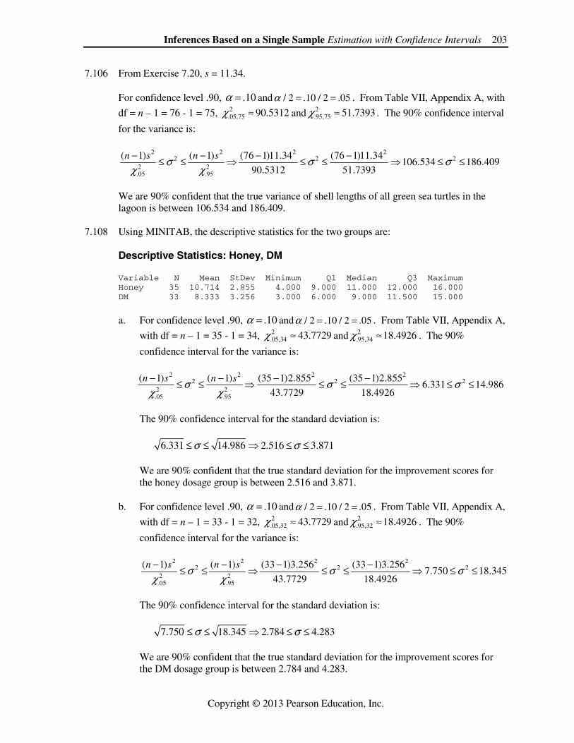
7.106 From Exercise 7.20, s = 11.34. For confidence level .90, .10α = and / 2 .10 / 2 .05α = = . From Table VII, Appendix A, with

df = n – 1 = 76 - 1 = 75, 2.05,75 90.5312χ ≈ and 2

.95,75 51.7393χ ≈ . The 90% confidence interval

for the variance is:

2 2 2 2

2 2 22 2.05 .95

( 1) ( 1) (76 1)11.34 (76 1)11.34106.534 186.409

90.5312 51.7393

n s n sσ σ σχ χ− − − −≤ ≤ ⇒ ≤ ≤ ⇒ ≤ ≤

We are 90% confident that the true variance of shell lengths of all green sea turtles in the

lagoon is between 106.534 and 186.409. 7.108 Using MINITAB, the descriptive statistics for the two groups are:

Descriptive Statistics: Honey, DM

Variable N Mean StDev Minimum Q1 Median Q3 Maximum Honey 35 10.714 2.855 4.000 9.000 11.000 12.000 16.000 DM 33 8.333 3.256 3.000 6.000 9.000 11.500 15.000

a. For confidence level .90, .10α = and / 2 .10 / 2 .05α = = . From Table VII, Appendix A,

with df = n – 1 = 35 - 1 = 34, 2.05,34 43.7729χ ≈ and 2

.95,34 18.4926χ ≈ . The 90%


2 2 2 2

2 2 22 2.05 .95

( 1) ( 1) (35 1)2.855 (35 1)2.8556.331 14.986

43.7729 18.4926

n s n sσ σ σχ χ− − − −≤ ≤ ⇒ ≤ ≤ ⇒ ≤ ≤


6.331 14.986 2.516 3.871σ σ≤ ≤ ⇒ ≤ ≤

We are 90% confident that the true standard deviation for the improvement scores for the honey dosage group is between 2.516 and 3.871.

b. For confidence level .90, .10α = and / 2 .10 / 2 .05α = = . From Table VII, Appendix A,

with df = n – 1 = 33 - 1 = 32, 2.05,32 43.7729χ ≈ and 2

.95,32 18.4926χ ≈ . The 90%


2 2 2 22 2 2

2 2.05 .95

( 1) ( 1) (33 1)3.256 (33 1)3.2567.750 18.345

43.7729 18.4926

n s n sσ σ σχ χ− − − −≤ ≤ ⇒ ≤ ≤ ⇒ ≤ ≤


7.750 18.345 2.784 4.283σ σ≤ ≤ ⇒ ≤ ≤

We are 90% confident that the true standard deviation for the improvement scores for the DM dosage group is between 2.784 and 4.283.

204 Chapter 7


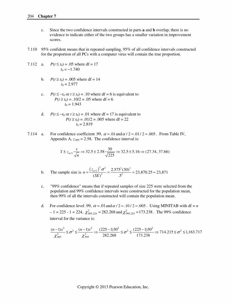
c. Since the two confidence intervals constructed in parts a and b overlap, there is no evidence to indicate either of the two groups has a smaller variation in improvement scores.

7.110 95% confident means that in repeated sampling, 95% of all confidence intervals constructed

for the proportion of all PCs with a computer virus will contain the true proportion. 7.112 a. P(t ≤ t0) = .05 where df = 17 t0 = −1.740 b. P(t ≥ t0) = .005 where df = 14 t0 = 2.977 c. P(t ≤ −t0 or t ≥ t0) = .10 where df = 6 is equivalent to P(t ≥ t0) = .10/2 = .05 where df = 6 t0 = 1.943 d. P(t ≤ −t0 or t ≥ t0) = .01 where df = 17 is equivalent to P(t ≥ t0) = .01/2 = .005 where df = 22 t0 = 2.819 7.114 a. For confidence coefficient .99, .01α = and / 2 .01 / 2 .005α = = . From Table IV,


/2

3032.5 2.58 32.5 5.16 (27.34, 37.66)

225

sx z

nα± ⇒ ± ⇒ ± ⇒

b. The sample size is ( )2 2 2 2

/22 2

2.575 (30)23,870.25 23,871

( ) .5

zn

SEα σ

= = = ≈

c. "99% confidence" means that if repeated samples of size 225 were selected from the

population and 99% confidence intervals were constructed for the population mean, then 99% of all the intervals constructed will contain the population mean.

d. For confidence level .99, .01α = and / 2 .10 / 2 .005α = = . Using MINITAB with df = n

– 1 = 225 - 1 = 224, 2.005,224 282.268χ = and 2

.995,224 173.238χ = . The 99% confidence

interval for the variance is:

2 2 2 22 2 2

2 2.005 .995

( 1) ( 1) (225 1)30 (225 1)30714.215 1,163.717

282.268 173.238

n s n sσ σ σχ χ− − − −≤ ≤ ⇒ ≤ ≤ ⇒ ≤ ≤



7.116 a. The point estimate for the mean personal network size of all older adults is 14.6x = . b. For confidence coefficient .95, .05α = and / 2 .05 / 2 .025α = = . From Table IV,


.025

9.81.96 14.6 1.96 14.6 .36 (14.24, 14.96)

2,819xx z x

n

σσ± ⇒ ± ⇒ ± ⇒ ± ⇒

c. We are 95% confident that the mean personal network size of all older adults is between

14.24 and 14.96. d. We must assume that we have a random sample from the target population and that the

sample size is sufficiently large. 7.118 Using MINITAB, the descriptive statistics are:

Descriptive Statistics: Commitment

Variable N Mean StDev Minimum Q1 Median Q3 Maximum Commitment 30 79.67 10.25 44.00 76.25 81.50 86.25 97.00

a. The point estimate for the mean charitable commitment of tax-exempt organizations is

79.67x = . b. For confidence coefficient .95, .05α = and / 2 .05 / 2 .025α = = . From Table IV,


/2

10.2579.67 1.96 79.67 3.67 (76.00, 83.34)

30

sx z

nα± ⇒ ± ⇒ ± ⇒

c. Since the sample size is at least 30, the Central Limit Theorem applies. We must

assume that we have a random sample from the population. d. The probability of estimating the true mean charitable commitment exactly with a point

estimate is zero. By using a range of values to estimate the mean (i.e. confidence interval), we can have a level of confidence that the range of values will contain the true mean.

e. For confidence level .95, .05α = and / 2 .05 / 2 .025α = = . From Table VII, Appendix

A, with df = n – 1 = 30 - 1 = 29, 2.025,29 45.7222χ = and 2

.975,29 16.0471χ = . The 95%


2 2 2 22 2 2

2 2.025 .975

( 1) ( 1) (30 1)10.25 (30 1)10.2566.637 189.867

45.7222 16.0471

n s n sσ σ σχ χ− − − −≤ ≤ ⇒ ≤ ≤ ⇒ ≤ ≤

We are 95% confident that the true variance of all charitable commitments for all tax-

exempt organizations is between 66.637 and 189.867.

206 Chapter 7


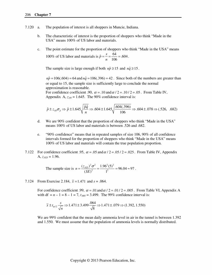
7.120 a. The population of interest is all shoppers in Muncie, Indiana.

b. The characteristic of interest is the proportion of shoppers who think “Made in the USA” means 100% of US labor and materials.

c. The point estimate for the proportion of shoppers who think “Made in the USA” means

100% of US labor and materials is64

ˆ .604106

xp

n= = = .

The sample size is large enough if both ˆ 15np ≥ and ˆ 15nq ≥ . ˆ 106(.604) 64np = = and ˆ 106(.396) 42nq = = . Since both of the numbers are greater than

or equal to 15, the sample size is sufficiently large to conclude the normal approximation is reasonable. For confidence coefficient .90, .10α = and / 2 .10 / 2 .05α = = . From Table IV, Appendix A, z.05 = 1.645. The 90% confidence interval is:

ˆ.05

ˆ ˆ .604(.396)ˆ ˆ 1.645 .604 1.645 .604 .078 (.526, .682)

106p

pqp z p

nσ± ⇒ ± ⇒ ± ⇒ ± ⇒

d. We are 90% confident that the proportion of shoppers who think “Made in the USA”

means 100% of US labor and materials is between .526 and .682. e. “90% confidence” means that in repeated samples of size 106, 90% of all confidence

intervals formed for the proportion of shoppers who think “Made in the USA” means 100% of US labor and materials will contain the true population proportion.

7.122 For confidence coefficient .95, .05α = and / 2 .05 / 2 .025α = = . From Table IV, Appendix

A, z.025 = 1.96.


.0252 2

( ) 1.96 (5)96.04 97

( ) 1

zn

SE

σ= = = ≈ .

7.124 From Exercise 2.184, 1.471x = and s = .064. For confidence coefficient .99, .01α = and / 2 .01 / 2 .005α = = . From Table VI, Appendix A

with df = n – 1 = 8 – 1 = 7, t.005 = 3.499. The 99% confidence interval is:

/2

.0641.471 3.499 1.471 .079 (1.392, 1.550)

8

sx t

nα± ⇒ ± ⇒ ± ⇒

We are 99% confident that the mean daily ammonia level in air in the tunnel is between 1.392

and 1.550. We must assume that the population of ammonia levels is normally distributed.



7.126 a. The point estimate of p is 39

ˆ .26150

xp

n= = = .

b. The sample size is large enough if both ˆ 15np ≥ and ˆ 15nq ≥ . 39)26(.150ˆ ==pn and 111)74(.150ˆ ==qn . Since both of the numbers are greater than

or equal to 15, the sample size is sufficiently large to conclude the normal approximation is reasonable.



.025

ˆ ˆ .26(.74)ˆ .26 1.96 .26 .070 (.190, .330)

150

pqp z

n± ⇒ ± ⇒ ± ⇒

c. We are 95% confident that the true proportion of college students who experience

"residual anxiety" from a scary TV show or movie is between .190 and .330. 7.128 Some preliminary calculations are:

160.97.314

22

xx

n= = =∑

( )1112.10

12222

9.1601.389,1

1

22

2

2 =−

−=

−

−=∑ ∑

nn

xx

s

180.31112.10 ==s

For confidence coefficient .95, .05α = and / 2 .05 / 2 .025α = = . From Table VI, Appendix A with df = n – 1 = 22 – 1 = 21, t.025 = 2.080. The 95% confidence interval is:

)724.8,904.5(410.1314.722

180.3080.2314.72/ ⇒±⇒±⇒±

n

stx α

We are 95% confident that the mean PMI for all human brain specimens obtained at autopsy

is between 5.904 and 8.724. Since 10 is not in the 95% confidence interval, it is not a likely value for the true mean. We

would infer that the true mean PMI for all human brain specimens obtained at autopsy is less than 10 days.

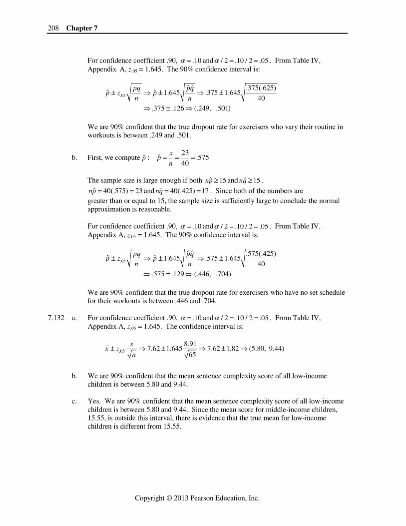
7.130 a. First, we compute p̂ : 15

ˆ .37540

xp

n= = =

The sample size is large enough if both ˆ 15np ≥ and ˆ 15nq ≥ . 15)375(.40ˆ ==pn and 25)625(.40ˆ ==qn . Since both of the numbers are greater than or equal to 15, the sample size is sufficiently large to conclude the normal approximation is reasonable.

208 Chapter 7



.05

ˆ ˆ .375(.625)ˆ ˆ 1.645 .375 1.645

40.375 .126 (.249, .501)

pq pqp z p

n n± ⇒ ± ⇒ ±

⇒ ± ⇒

We are 90% confident that the true dropout rate for exercisers who vary their routine in

workouts is between .249 and .501.

b. First, we compute p̂ : 575.40

23ˆ ===

n

xp

The sample size is large enough if both 15ˆ ≥pn and 15ˆ ≥qn .

23)575(.40ˆ ==pn and 17)425(.40ˆ ==qn . Since both of the numbers are greater than or equal to 15, the sample size is sufficiently large to conclude the normal approximation is reasonable. For confidence coefficient .90, .10α = and / 2 .10 / 2 .05α = = . From Table IV,


.05

ˆ ˆ .575(.425)ˆ ˆ 1.645 .575 1.645

40.575 .129 (.446, .704)

pq pqp z p

n n± ⇒ ± ⇒ ±

⇒ ± ⇒

We are 90% confident that the true dropout rate for exercisers who have no set schedule

for their workouts is between .446 and .704. 7.132 a. For confidence coefficient .90, .10α = and / 2 .10 / 2 .05α = = . From Table IV,


.05

8.917.62 1.645 7.62 1.82 (5.80, 9.44)

65

sx z

n± ⇒ ± ⇒ ± ⇒

b. We are 90% confident that the mean sentence complexity score of all low-income children is between 5.80 and 9.44.

c. Yes. We are 90% confident that the mean sentence complexity score of all low-income

children is between 5.80 and 9.44. Since the mean score for middle-income children, 15.55, is outside this interval, there is evidence that the true mean for low-income children is different from 15.55.



7.134 a. For confidence coefficient .95, .05α = and / 2 .05 / 2 .025α = = . From Table VI, Appendix A, with df = n − 1 = 15 − 1 = 14, t.025 = 2.145. The confidence interval is:

.025

1.515.87 2.145 5.87 .836 (5.034, 6.706)

15

sx t

n± ⇒ ± ⇒ ± ⇒

We are 95% confident that the true mean response of the students is between 5.034 and 6.706.

b. In part a, the width of the interval is 6.706 − 5.034 = 1.672. The value of SE is 1.672/2

= .836. If we want the interval to be half as wide, the value of SE would be half that in part a or .836/2 = .418. The necessary sample size is:

2 2 2 2

/22 2

1.96 1.5150.13 51

( ) .418

zn

SEα σ= = = ≈

7.136 For confidence coefficient .95, .05α = and / 2 .05 / 2 .025α = = . From Table IV, Appendix

A, z.025 = 1.96. From Exercise 7.107, a good approximation for p is .094.

The sample size is ( )2 2

/22 2

(1.96) (.094)(.906)817.9 818

( ) .02

z pqn

SEα= = = ≈

You would need to take n = 818 samples. 7.138 The sample size is large enough if both ˆ 15np ≥ and ˆ 15nq ≥ . ˆ 150(.11) 16.5np = = and ˆ 150(.89) 133.5nq = = . Since both of the numbers are greater than or

equal to 15, the sample size is sufficiently large to conclude the normal approximation is reasonable.


.025

ˆ ˆ .11(.89)ˆ ˆ 1.96 .11 1.96 .11 .050 (.06, .16)

150

pq pqp z p

n n± ⇒ ± ⇒ ± ⇒ ± ⇒

We are 95% confident that the true proportion of all MSDS that are satisfactorily completed

is between .06 and .16. Yes. Since 20% or .20 is not contained in the confidence interval, it is not a likely value.

7.140 a. The point estimate of p is35

ˆ .63655

xp

n= = = .

The sample size is large enough if both ˆ 15np ≥ and ˆ 15nq ≥ .

210 Chapter 7


ˆ 55(.636) 35np = = and ˆ 55(.364) 20nq = = . Since both of the numbers are greater than or equal to 15, the sample size is sufficiently large to conclude the normal approximation is reasonable.

Since no level of confidence is given, we will use 95% confidence. For confidence

coefficient .95, .05α = and / 2 .05 / 2 .025α = = . From Table IV, Appendix A, z.025 = 1.96. The 95% confidence interval is:

.025

ˆ ˆ .636(.364)ˆ ˆ 1.96 .636 1.96 .636 .127 (.509, .763)

55

pq pqp z p

n n± ⇒ ± ⇒ ± ⇒ ± ⇒

We are 95% confident that the true proportion of all fatal air bag accidents involving children is between .509 and .763.

b. The sample proportion of children killed by air bags who were not wearing seat belts or

were improperly restrained is 24/35 = .686. This is a rather large proportion. Whether a child is killed by an air bag could be related to whether or not he/she was properly restrained. Thus, the number of children killed by air bags could possibly be reduced if the child were properly restrained.

Documents

Chapter 7 Chapter Inferences Based on a Single Sample ... Based on a Single Sample Estimation with Confidence ... the descriptive statistics are: ... on a Single Sample Estimation