CHAPTER-7

CASE STUDY

The study was conducted at a manufacturing facility specializing in plastic

products. The particular plant is a part of the “parag group” of its parent

company, which is made up of three divisions: filter, hygiene/medical, and

plastics. This company‟s vision, which is to be innovative and quality-driven in

its technically demanding applications, is determined by its guiding principles of

continuous improvement, leadership, and commitment to anticipate and

understand their customer‟s needs and expectations. Seventy percent of the

plant‟s revenue comes from the plastic moulded parts, it produces for the

automotive industry.

The proposed DAURR (Diagnose, Analyze, Upgrade, Regulate and Review)

principle along with various statistical tools of six sigma was applied to improve

the quality of nylon-6 bush (KAMANI BUSH) produced by plastic injection

moulding process. The production equipment employed in this study was a

precision injection machine, model: PPU7690TV40G, over all dimensions

856×1500×2480 mm manufactured by the Targor Corporation. This machine

was installed at Central Institute of Plastic Engineering and Technology

(CIPET) Lucknow.

7.1. MODIFIED METHODOLOGY FOR SMALL ENTERPRISES

Having arisen in large corporations, Six Sigma is surely one of the most

comprehensive approaches for company development and performance

improvement of products and processes. Nevertheless, it appears that the

majority of small and medium sized enterprises (SMEs) either does not know

the six sigma approach, or find its organization not suitable to meet their specific

requirements. In the SME environment, there is little spare resource; every

employee has a key role and usually several [Ryan‟s, 1995, cited by Macadam,

2000].

The challenges of smaller companies are “funding and logistics”, a “limited

talent pool”, “multi-hat roles”, and “less exposure to management innovations in

other industries”.

However the other side of the coin is that it is easier to implement TQM in

SMEs because the power of decision making does not depend on extensive

hierarchies but lies within the owner managers.

Since the SMEs have a much closer proximity to the customers and this

proximity is coupled with a larger number of SME employees having direct

customer contact and knowledge “therefore, the customer voice can be

incorporated within SME operations without prolonged and formalized

approaches” [Hale and Cragg, 1996, cited by McAdam, 2000].

Traditional loyalty to specific customers ,support improvement efforts, which

are visible to the customers. Six Sigma depends on reliable ways of collecting

the voices of the customer and translating these into critical-to-quality

requirements of products and services. This close relationship and the high

degree of communication with key customers appear to be significant

advantages of SMEs in opposition to large corporations.

The review of published literature on general QM and the cultural requirements

that build the basis for any Six Sigma program, combined with the survey

responses, suggest that several factors have to be represented in a Six Sigma

initiative within an SME context. These are

(1) The Six Sigma roles should be restricted to the project leaders in the SME

organisation (e.g. an “SME black belt”). The rest of the workforce and

management staff should only participate in the awareness training.

(2) A general six sigma concept for SMEs needs to be adjusted to the core

requirements of ISO 9000 to enable a certification, which represents a major

difference to Six Sigma programs in large corporations.

(3) A training program has to be employed which is significantly shorter than in

large corporations, but is still based on the well-proven methods and tools of

QM adjusted to specific SME needs.

(4) SMEs require consulting services which differ significantly from those

usually found in the Market place working for larger corporations. SMEs require

consultants and trainers offering modular services, which allow the addition or

subtraction of elements without compromising the entirety of the concept and

without risking the success for their target group.

Keeping in mind the above problems and specific requirements of SMEs

,especially the plastic injection moulding industry, the DMAIC procedure of six

sigma can be moulded into a cycle with slight modification.

Fig.7.1 Modified approach in a cycle

The road map of this new proposed method is given in the Table 7.1. Based on

this modified methodology a case study was carried in a small enterprise

consisting of one expert (Black Belt) and few trained personnel. The results of

this case study are discussed further in the article which are quite satisfactory.

This modified approach will not put a large financial burden on small scale

industries having, limited talent pool and less exposure to management

innovations. The approach will help them to upgrade their existing system in a

slow but steady manner. The experimental work was done at Central Institute of

Plastic Engineering and Technology (CIPET), Lucknow.

Table-7.1 Road map for the proposed methodology

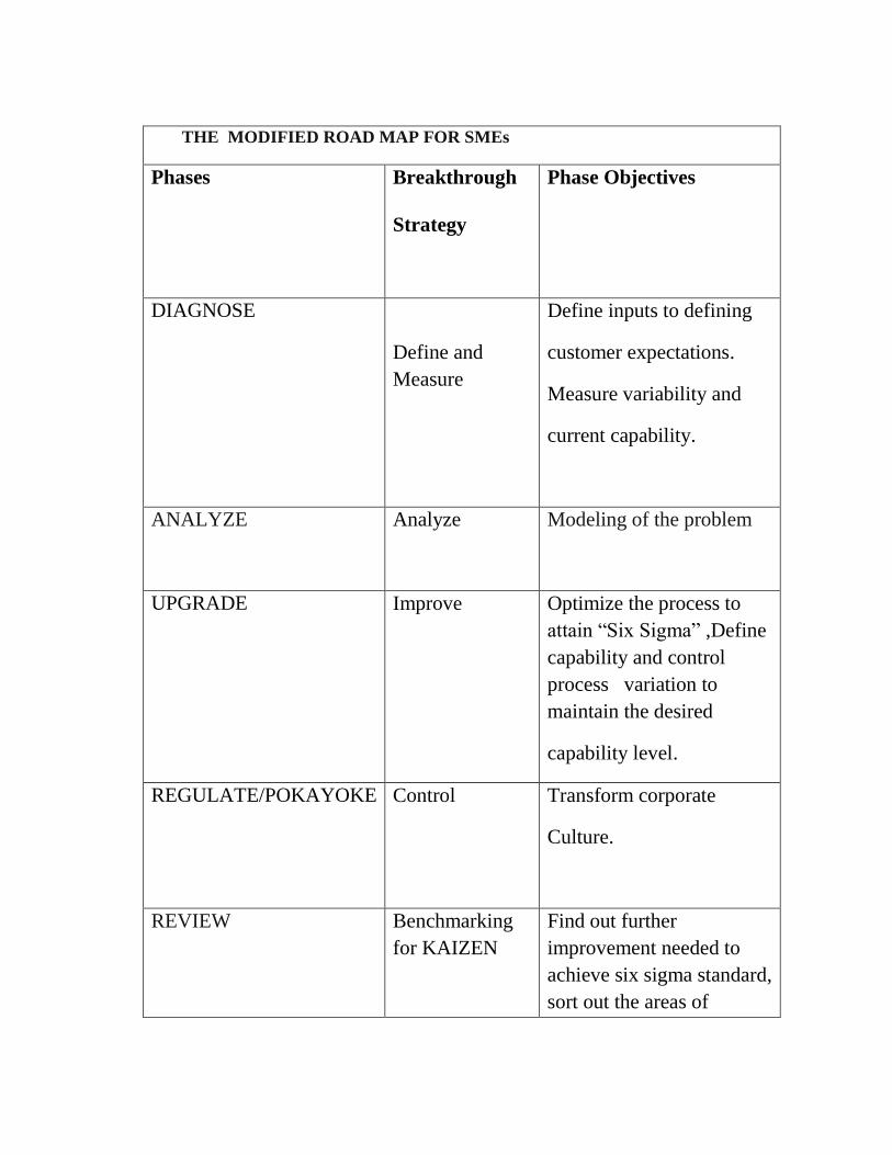
THE MODIFIED ROAD MAP FOR SMEs

Phases

Breakthrough

Strategy

Phase Objectives

DIAGNOSE

Define and

Measure

Define inputs to defining

customer expectations.

Measure variability and

current capability.

ANALYZE Analyze

Modeling of the problem

UPGRADE

Improve Optimize the process to

attain “Six Sigma” ,Define

capability and control

process variation to

maintain the desired

capability level.

REGULATE/POKAYOKE

Control

Transform corporate

Culture.

REVIEW Benchmarking

for KAIZEN

Find out further

improvement needed to

achieve six sigma standard,

sort out the areas of

improvement whether

Man,Machine,Material or

Method, Switch to

diagnose stage.

Nylon-6 bush (KAMANI BUSH) produced by plastic injection moulding

process has following specifications.

Length- 44.4mm, internal diameter-16.1mm, Outer diameter-22mm.

Fig.7.2 Drawing of nylon-6 bush

Application of modified methodology at manufacturing facility is described

below

7.2 DIAGNOSE

The first step in modified procedures is to define and measure the problems so

that possible confusion in targets for improvement due to differences in

cognition among project staff can be avoided. In this phase, the reasons for

rejection and failure of nylon-6 bush were investigated by the management

techniques like voice of customer and brain storming of production manager,

quality engineer on the shop floor, as well as workers concerned with the

production of the above product. After voice of customer and brain storming we

concluded that following four defects were playing important role in rejection

and failure of the bush.

1. Sink marks 2. Stress cracking 3.Bulging defect (over shrinkage) 4.Low

value of hardness

After doing Pareto analysis we decided that bulging defect and low value of

hardness are responsible for 80% of the failures and rejection.

To measure the problem, the process capability index was ued to illustrate the

most efficient way to circumvent the problems defined in the previous steps

(bulging defect and hardness in this case). For the nylon-6 bush moulded in this

study, the process capability index is measured based upon the data obtained

from the bulging and hardness measurements (For the bulging measurement we

used a dial gauge attached with a V shaped anvil placed over a surface plate

while for the hardness measurement we used core hardness indenter).

In general, the upper process capability index CPU is defined by the following

equation.

CPU= USL- µ

3σ

Where USL is the upper specification limit, µ is the mean of all measured

values, and σ is the standard deviation.

Similarly the lower process capability index CPL is defined by the following

equation.

CPL= µ-LSL

3σ

Where LSL is the lower specification limit. The higher value of CPU or CPL is

known as Cpk.

Before implementation of six sigma projects hundred random samples were

taken from production line at ten different occasions in a week and over

shrinkage in samples was measured, using dial gauge attached with a V shaped

anvil, placed over a surface plate. SPC software was used to analyze the process.

Fig.7.3 Histogram for hundred random samples taken from production line at

ten different occasions in a week (over shrinkage measurements shown on x-

axis).

Value of CPL calculated from hundred random samples for over shrinkage was

0.24 and production was of 2.38 sigma standard and the process mean was

0.1015.Analysis indicates that 19% defects are expected. This is obvious from

the Fig.7.3 and Table-7.2.

Similarly SPC analysis for hardness was carried out with the help of hundred

samples taken from production line at ten different occasions in a week. The

histogram for these measurements is shown in Fig.7.4.

Value of CPU calculated from hundred random samples for hardness was 0.56

and production is of 3.19 sigma standard and the process mean was 69.79. This

is obvious from the Fig.7.4 and Table-7.3.

Table-7.2 SPC software analysis for over shrinkage (bulging defect) in selected

samples

Cp values Decimal Points 2.00

Cpk 0.24 Number of Entries 100

CpU 0.24 Average 0.1015

Ppk 0.23 Stdev 0.03

Min 0.05 Median 0.1

Max 0.15 Mode 0.12

Z Bench 0.71 Minimum Value 0.05

% Defects 19.0% Maximum Value 0.15

PPM 190000.00 Range 0.1

Expected 238713.25 USL 0.12

Sigma 2.38

Observed Expected Z

PPM<LSL * * *

PPM>USL 190000.0 238713.2 0.71

PPM 190000.0 238713.2

SPC analysis for hardness was carried out with the help of hundred samples

taken from production line at ten different occasions in a week. The histogram

for these measurements is shown in Fig. 7.4.

Hardness values

Fig.-7.4 Histogram for hardness of hundred samples (horizontal axis shows

hardness, vertical axis shows number of samples)

Table-7.3 SPC analysis for hardness in selected samples (for hardness

measurements)

Cp * Number of Entries 100

Cpk 0.56 Average 69.79

CpU * Stdev 2.77

CpL 0.56 Median 70

ZTarget/DZ 1.27 Mode 68

Pp * Minimum Value 65

Ppk 0.58 Maximum Value 76

Range 11

PpL 0.58 LSL 65

Skewness 0.19 USL FALSE

Stdev 2.771773 Number of Bars 10.00

Min 65 Number of Classes 10.00

Max 76 Class Width 1.10

Z Bench 1.69 Beginning Point 63.9

% Defects 0.0% Stdev Est 2.84

PPM 0.00 d2/c4 0.97

Expected 45568.98 Target 73.31532

Sigma 3.19

Observed Expected Z

PPM<LSL 0.0 45569.0 -1.69

PPM>USL * * *

PPM 0.0 45569.0

% Defects 0.0 0.0

7.3 ANALYZE

In the analysis step, the data collected from the process is analyzed in

accordance with the CTQ (critical to quality) factors. The literature review

suggests that to have better surface quality of moulded part, it is important to

correctly tune the settings of process parameters in injection moulding ,as well

as precision machining of mould.

Fig. 7.5 Cause-and-effect diagram shown in fishbone schematics for the

moulded bush.

There are many factors that influence the quality of the moulded bush but eight

factors are selected here as shown in bold italic type.

According to the literature and with the cause-and-effect diagram shown in

Fig.7.5, the most significant processing parameters selected were melt

temperature(A), injection pressure(B) injection speed(C), mold temperature(D),

packing pressure(E), packing time(F) , cooling time(G) and screw speed(H).

Using Taguchi method L27 orthogonal experiment was performed setting above

eight parameters at three different levels.

Table-7.4 Different parameters and their levels

Parameter Symbol Values at different levels

Level-1 Level-2 Level-3

Melting

temperature

A 2600C 275

0C 290

0C

Injection pressure B 60 M Pa 75 M Pa 90 M Pa

Injection speed C 40 Cm3/Sec 50 Cm

3/Sec 60

Cm3/Sec

Mold temperature D 40 0C 60

0C 80

0C

Packing pressure E 70 M Pa 75 M Pa 80 M Pa

Packing time F 3 Sec 4 Sec 5 Sec

Cooling time G 20 Sec 30 Sec 40 Sec

Screw speed H 50 rpm 65 rpm 80 rpm

S/N (signal to noise) ratio in Taguchi method is helpful in the selection of

process parameters at better levels. A large number of different S/N ratios have

been defined for a variety of problems, though in this work we have used larger

the better characteristic for hardness and smaller the better characteristic for

over shrinkage (bulging defect).The method used to calculate S/N ratio for both

the types is as follows:

7.3.1 Larger – the – better

S/N ratio (η) =−10 log10(1/n∑1/yi2) [ i=1 to n]

Where n = number of replications.

This is applied for problems where maximization of the quality characteristic of

interest is sought. This is referred to as the larger-the-better type problem.

7.3.2 Smaller – the – better

S/N ratio (η) =−10 log10(1/n∑ yi2) [ i=1 to n]

This is termed as smaller-the-better type problem where minimization of the

characteristic is intended.

Table-7.5 Average value of hardness (for three sample pieces) and S/N(signal to

noise) ratio in 27 experiments performed at three different levels of parameters

A, B, C, D, E, F, G, and H.

S.No.

A

B

C

D

E

F

G

H

Hardness S/N

ratio

1 1 1 1 1 1 1 1 1 75 37.5

2 1 1 1 1 2 2 2 2 77 37.73

3 1 1 1 1 3 3 3 3 76 37.62

4 1 2 2 2 1 1 1 2 74.5 37.44

5 1 2 2 2 2 2 2 3 78 37.84

6 1 2 2 2 3 3 3 1 76 37.62

7 1 3 3 3 1 1 1 3 80 38.06

8 1 3 3 3 2 2 2 1 81.33 38.21

9 1 3 3 3 3 3 3 2 80.5 38.12

10 2 1 2 3 1 2 3 1 80.5 38.12

11 2 1 2 3 2 3 1 2 83.66 38.45

12 2 1 2 3 3 1 2 3 81.66 38.24

13 2 2 3 1 1 2 3 2 81.5 38.22

14 2 2 3 1 2 3 1 3 84.66 38.55

15 2 2 3 1 3 1 2 1 83.66 38.45

16 2 3 1 2 1 2 3 3 79.66 38.02

17 2 3 1 2 2 3 1 1 82.66 38.35

18 2 3 1 2 3 1 2 2 81.5 38.22

19 3 1 3 2 1 3 2 1 82.66 38.35

20 3 1 3 2 2 1 3 2 84 38.49

21 3 1 3 2 3 2 1 3 84.33 38.52

22 3 2 1 3 1 3 2 2 82 38.28

23 3 2 1 3 2 1 3 3 83.66 38.45

24 3 2 1 3 3 2 1 1 81 38.17

25 3 3 2 1 1 3 2 3 78 37.84

26 3 3 2 1 2 1 3 1 80 38.06

27 3 3 2 1 3 2 1 2 79 37.95

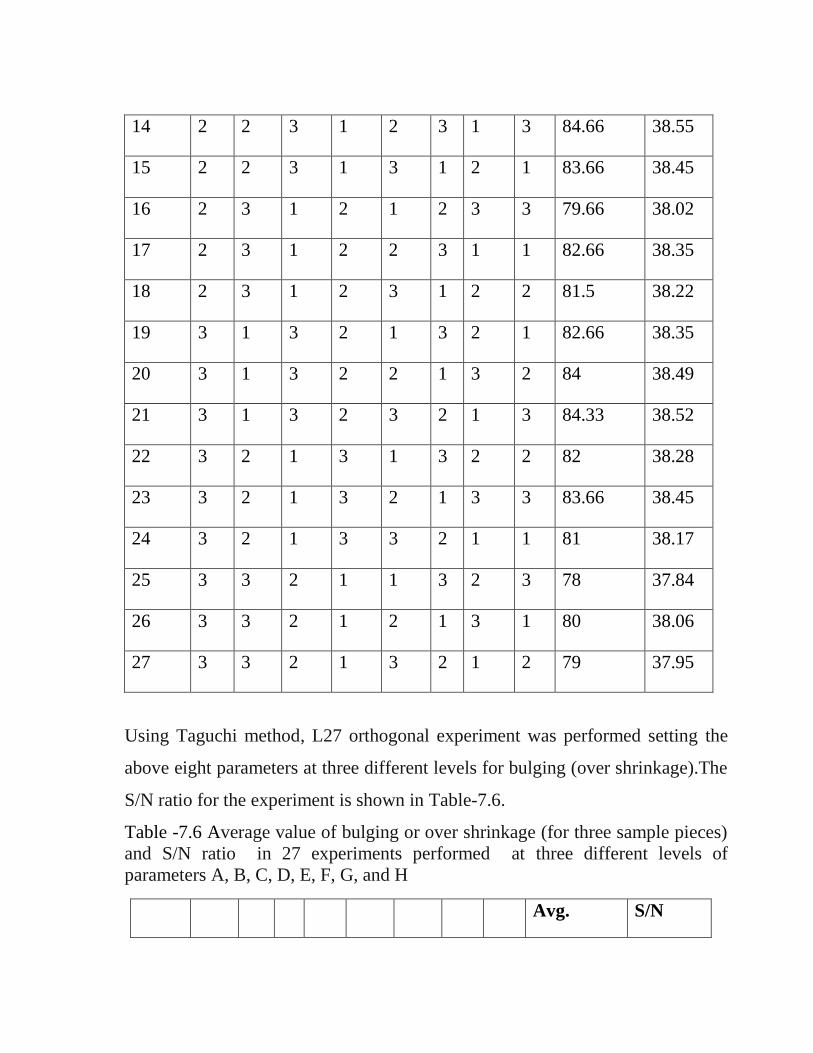
Using Taguchi method, L27 orthogonal experiment was performed setting the

above eight parameters at three different levels for bulging (over shrinkage).The

S/N ratio for the experiment is shown in Table-7.6.

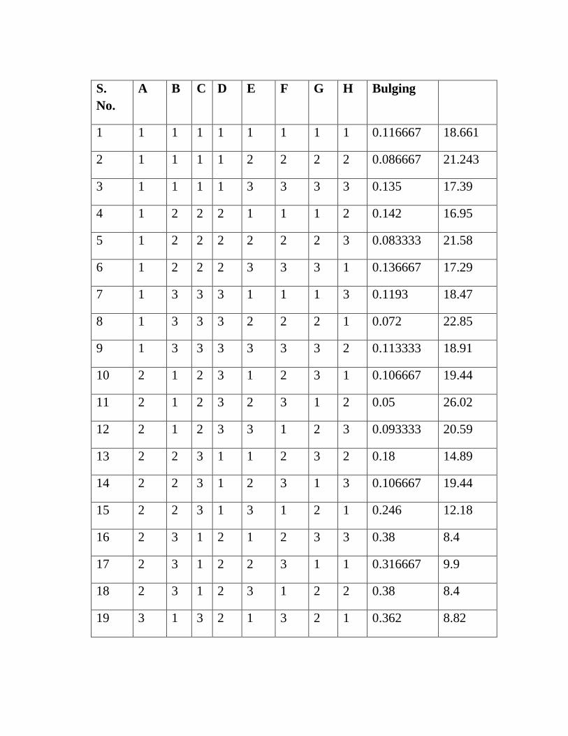
Table -7.6 Average value of bulging or over shrinkage (for three sample pieces)

and S/N ratio in 27 experiments performed at three different levels of

parameters A, B, C, D, E, F, G, and H

Avg. S/N

S.

No.

A B C D E F G H Bulging

1 1 1 1 1 1 1 1 1 0.116667 18.661

2 1 1 1 1 2 2 2 2 0.086667 21.243

3 1 1 1 1 3 3 3 3 0.135 17.39

4 1 2 2 2 1 1 1 2 0.142 16.95

5 1 2 2 2 2 2 2 3 0.083333 21.58

6 1 2 2 2 3 3 3 1 0.136667 17.29

7 1 3 3 3 1 1 1 3 0.1193 18.47

8 1 3 3 3 2 2 2 1 0.072 22.85

9 1 3 3 3 3 3 3 2 0.113333 18.91

10 2 1 2 3 1 2 3 1 0.106667 19.44

11 2 1 2 3 2 3 1 2 0.05 26.02

12 2 1 2 3 3 1 2 3 0.093333 20.59

13 2 2 3 1 1 2 3 2 0.18 14.89

14 2 2 3 1 2 3 1 3 0.106667 19.44

15 2 2 3 1 3 1 2 1 0.246 12.18

16 2 3 1 2 1 2 3 3 0.38 8.4

17 2 3 1 2 2 3 1 1 0.316667 9.9

18 2 3 1 2 3 1 2 2 0.38 8.4

19 3 1 3 2 1 3 2 1 0.362 8.82

20 3 1 3 2 2 1 3 2 0.303333 10.36

21 3 1 3 2 3 2 1 3 0.345 9.24

22 3 2 1 3 1 3 2 2 0.283333 10.95

23 3 2 1 3 2 1 3 3 0.234 12.61

24 3 2 1 3 3 2 1 1 0.28 11.05

25 3 3 2 1 1 3 2 3 0.182 14.79

26 3 3 2 1 2 1 3 1 0.13 17.72

27 3 3 2 1 3 2 1 2 0.175 15.14

Table-7.7 Average values of S/N ratio at different parameter levels

S. NO. Parameter

Levels

Avg. S/N

ratio

(Bulging)

Parameter

Levels

Avg. S/N

ratio

(Hardness)

1 A1 19.26 A1 37.7933

2 A2 15.47 A2 38.2911

3 A3 12.3 A3 38.2344

4 B1 16.86 B1 38.11333

5 B2 16.66 B2 38.11333

6 B3 14.95 B3 38.09222

7 C1 13.18 C1 38.03778

8 C2 18.84 C2 37.95111

9 C3 15.02 C3 38.33

10 D1 16.83 D1 37.9911

11 D2 12.33 D2 38.0944

12 D3 17.88 D3 38.2333

13 E1 14.59 E1 37.9811

14 E2 17.96 E2 38.2366

15 E3 14.47 E3 38.10111

16 F1 15.11 F1 38.10111

17 F2 15.98 F2 38.08667

18 F3 15.94 F3 38.1311

19 G1 16.09 G1 38.11

20 G2 15.71 G2 38.12889

21 G3 15.22 G3 38.08

22 H1 15.32 H1 38.0922

23 H2 15.87 H2 38.1

24 H3 15.83 H3 38.12667

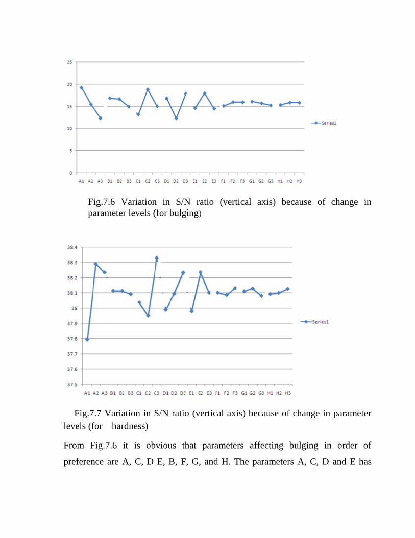
Fig.7.6 Variation in S/N ratio (vertical axis) because of change in

parameter levels (for bulging)

Fig.7.7 Variation in S/N ratio (vertical axis) because of change in parameter

levels (for hardness)

From Fig.7.6 it is obvious that parameters affecting bulging in order of

preference are A, C, D E, B, F, G, and H. The parameters A, C, D and E has

larger impact on the bulging defect therefore these parameters were selected to

make regression and neural network models.

While Fig.7.7 depicts that parameters affecting hardness in order of preference

are A, C, E, D, G, F, H, B. The parameters A, C, E and D have larger impact on

the hardness therefore these parameters were selected to make regression and

neural network models.

Both the properties hardness and bulging are affected the most by the parameters

A, C, D and E therefore these will be considered for further analysis.

The first order regression equation with the above variables did not give better

results; therefore we opted for second order regression analysis.

With the help of the above data we formed a second order regression equation

for hardness as below

HARD = 6.3732839507248 A +0.012305555556039 D -2.0035555555469 C

+10.93255555366 E -0.011343209876806 A2 +0.00034861111110563 D

2

+0.021377777777698C2 -0.072155555545211 E

2 -1182.3028394404 + e

……………………. (1)

Where „e‟ is an error term

The regression statics for this model is depicted in Table-7.8

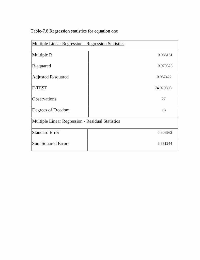
Table-7.8 Regression statistics for equation one

Multiple Linear Regression - Regression Statistics

Multiple R 0.985151

R-squared 0.970523

Adjusted R-squared 0.957422

F-TEST 74.079898

Observations 27

Degrees of Freedom 18

Multiple Linear Regression - Residual Statistics

Standard Error 0.606962

Sum Squared Errors 6.631244

Table-7.9 Regression statistics (Analysis of Variance) for equation (1)

Multiple Linear Regression - Analysis of Variance

ANOVA DF Sum of Squares Mean

Square

Regression 8 218.329741 27.291218

Residual 18 6.631244 0.368402

Total 26 224.960985 8.6523455840456

F-TEST 74.079898

Table-7.10 Regression statistics (Student Distribution Probability) for equation

(1)

Student Distribution Probability

(mathematical equation plotter)

T-Test 10.5206

D.F. 18

Fig.7.8 Comparison between actual hardness values (dotted) and predicted

hardness values (from equation one) for twenty seven experimental

samples.

Fig.7.9 Residuals plot for twenty seven experimental samples.

Similarly the second order regression equation for bulging was formed as below

BULGING = 0.061682428194518 A +0.0364504629528 D -0.10546870372806

C -0.33662925904979 E -0.0001034650209666 A2 -0.00030389351847241 D

2

+0.001034425926114 C2 +0.0022465925911414 E

2 +5.2475707471113 +

e………….. (2)

The Regression Statistics of this model is shown in table-7.11.

Table-7.11 Regression statistics for bulging model shown in equation (2)

Multiple Linear Regression - Regression Statistics

Multiple R

0.984221

R-squared

0.968691

Adjusted R-squared

0.954776

F-TEST

69.614348

Observations

27

Degrees of Freedom

18

Multiple Linear Regression - Residual Statistics

Standard Error 0.022217

Table-7.12 Analysis of Variance for bulging model shown by equation (2)

Multiple Linear Regression - Analysis of Variance

ANOVA DF Sum of Squares Mean Square

Regression 8 0.274894 0.034362

Residual 18 0.008885 0.000494

Total 26 0.283779 0.010914588545104

F-TEST 69.614348

Table-7.13 Student Distribution Probability for bulging model shown by

equation (2)

Student Distribution Probability

(mathematical equation plotter)

T-Test 2.7817

D.F. 18

Fig.7.10 Comparison between actual shrinkage values (dotted) and predicted

shrinkage values for twenty seven experimental samples.

Fig.7.11 Residuals plot for twenty seven experimental samples.

These second order regression models were further validated with the help of

neural network models which have been prepared separately for both hardness

and bulging predictions.

The twenty seven results of Table-7.5 were used for training neural network

model. We used neural net work model with following specifications for

prediction of hardness value

Minimum weight-0.0001

Limit of epochs-10,000

Initial weight-0.3

Learning rate -0.3

Momentum-0.6

Activation function –Log sigmoid function with no neurons in hidden layer

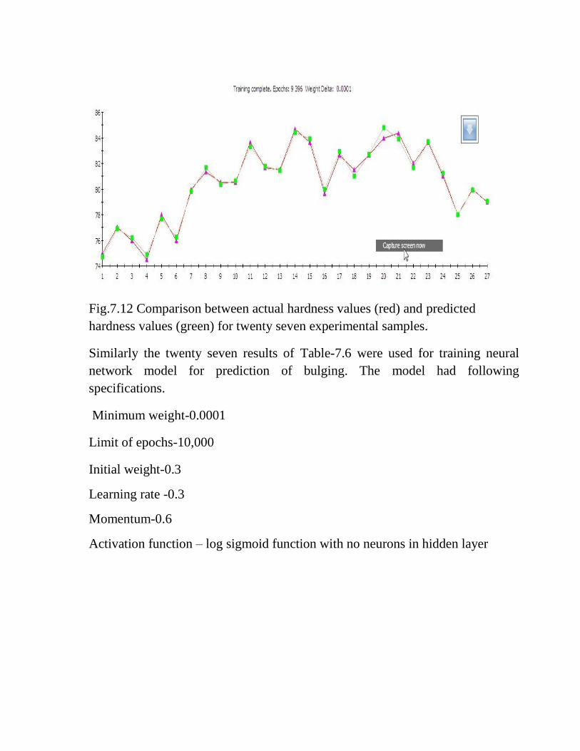
Fig.7.12 Comparison between actual hardness values (red) and predicted

hardness values (green) for twenty seven experimental samples.

Similarly the twenty seven results of Table-7.6 were used for training neural

network model for prediction of bulging. The model had following

specifications.

Minimum weight-0.0001

Limit of epochs-10,000

Initial weight-0.3

Learning rate -0.3

Momentum-0.6

Activation function – log sigmoid function with no neurons in hidden layer

Fig.7.13 Comparison between actual shrinkage values (red) and predicted

shrinkage values (green) for twenty seven experimental samples.

From Fig.7.6 and Fig.7.7 it is obvious that factors A, D, C and E has the most

significant affect on both the quality characteristics i.e. over shrinkage and

hardness. Taguchi design of experiment (Table-7.5 and Table-7.6) indicates that

hardness is maximum when parameters are at A2, C3, D1 and E2 levels while

over shrinkage is minimum when parameters are at A2, C2, D3 and E2 levels.

Since the parameters A and E give optimum value of both the quality

characteristics at the same level a compromise was made between parameters C

and D with the help of regression and neural net work models prepared with the

help of experiment.

The predicted values of hardness and over shrinkage (bulging) at different

values of parameters A, C, D and E are shown in Table-7.14.After analyzing the

predicted values of hardness and over shrinkage, obtained from both the models,

we selected parameter A-275, D-80, C-54 and E-75, which shows best

compromise between hardness and over shrinkage.

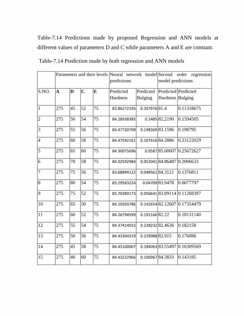
Table-7.14 Predictions made by proposed Regression and ANN models at

different values of parameters D and C while parameters A and E are constant.

Table-7.14 Prediction made by both regression and ANN models

Parameters and their levels Neural network model

predictions

Second order regression

model predictions

S.NO. A D C E Predicted

Hardness

Predicted

Bulging

Predicted

Hardness

Predicted

Bulging

1 275 45 52 75 83.86272195 0.207976 81.4 0.11318675

2 275 50 54 75 84.28938385 0.2485 82.2190 0.1594505

3 275 55 56 75 84.47720709 0.198369 83.1596 0.198795

4 275 60 58 75 84.47592161 0.107416 84.2886 0.23122029

5 275 65 60 75 84.30075696 0.0587 85.60607 0.25672627

6 275 70 58 75 84.02592984 0.052041 84.86487 0.2006633

7 275 75 56 75 83.68894122 0.048561 84.3121 0.1376811

8 275 80 54 75 83.29563224 0.04709 83.9478 0.0677797

9 275 75 52 75 83.70390173 0.056641 83.09114 0.11268397

10 275 65 50 75 84.10593786 0.142654 82.12607 0.17354479

11 275 60 52 75 84.26794599 0.192166 82.22 0.18131140

12 275 55 54 75 84.37414015 0.228232 82.4636 0.182158

13 275 50 56 75 84.43304319 0.229088 82.915 0.176086

14 275 45 58 75 84.45100007 0.184063 83.55497 0.16309569

15 275 40 60 75 84.43222966 0.106967 84.3833 0.143185

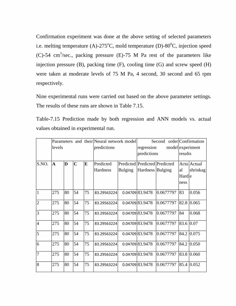
Confirmation experiment was done at the above setting of selected parameters

i.e. melting temperature (A)-275oC, mold temperature (D)-80

0C, injection speed

(C)-54 cm3/sec., packing pressure (E)-75 M Pa rest of the parameters like

injection pressure (B), packing time (F), cooling time (G) and screw speed (H)

were taken at moderate levels of 75 M Pa, 4 second, 30 second and 65 rpm

respectively.

Nine experimental runs were carried out based on the above parameter settings.

The results of these runs are shown in Table 7.15.

Table-7.15 Prediction made by both regression and ANN models vs. actual

values obtained in experimental run.

Parameters and their

levels

Neural network model

predictions

Second order

regression model

predictions

Confirmation

experiment

results

S.NO. A D C E Predicted

Hardness

Predicted

Bulging

Predicted

Hardness

Predicted

Bulging

Actu

al

Hard

ness

Actual

shrinkag

e

1 275 80 54 75 83.29563224 0.04709 83.9478 0.0677797 83 0.056

2 275 80 54 75 83.29563224 0.04709 83.9478 0.0677797 82.8 0.065

3 275 80 54 75 83.29563224 0.04709 83.9478 0.0677797 84 0.068

4 275 80 54 75 83.29563224 0.04709 83.9478 0.0677797 83.6 0.07

5 275 80 54 75 83.29563224 0.04709 83.9478 0.0677797 84.2 0.075

6 275 80 54 75 83.29563224 0.04709 83.9478 0.0677797 84.2 0.050

7 275 80 54 75 83.29563224 0.04709 83.9478 0.0677797 83.8 0.060

8 275 80 54 75 83.29563224 0.04709 83.9478 0.0677797 85.4 0.052

9 275 80 54 75 83.29563224 0.04709 83.9478 0.0677797 84.6 0.062

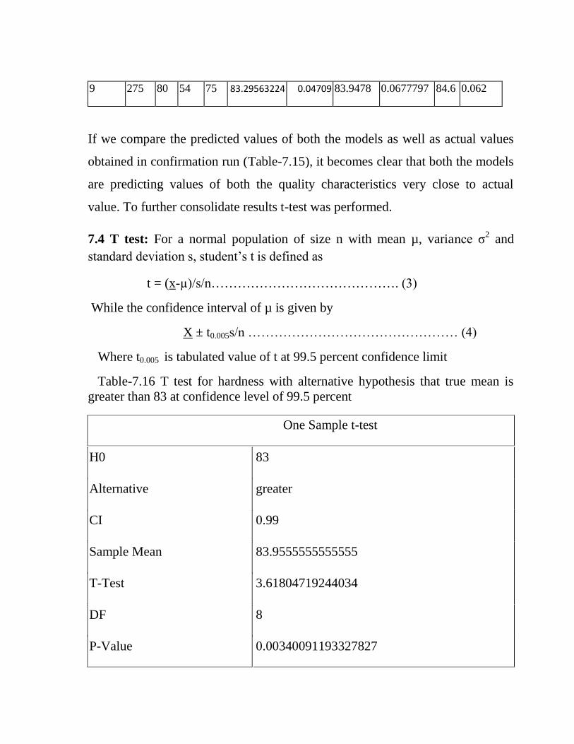
If we compare the predicted values of both the models as well as actual values

obtained in confirmation run (Table-7.15), it becomes clear that both the models

are predicting values of both the quality characteristics very close to actual

value. To further consolidate results t-test was performed.

7.4 T test: For a normal population of size n with mean µ, variance σ2 and

standard deviation s, student‟s t is defined as

t = (x-µ)/s/n……………………………………. (3)

While the confidence interval of µ is given by

X ± t0.005s/n ………………………………………… (4)

Where t0.005 is tabulated value of t at 99.5 percent confidence limit

Table-7.16 T test for hardness with alternative hypothesis that true mean is

greater than 83 at confidence level of 99.5 percent

One Sample t-test

H0 83

Alternative greater

CI 0.99

Sample Mean 83.9555555555555

T-Test 3.61804719244034

DF 8

P-Value 0.00340091193327827

Since the p value is smaller than significance level and tabulated value of t

(3.355) is less than calculated value (3.61804) null hypothesis that actual mean

is 83 is rejected and alternate hypothesis that actual sample mean is more than

83 is accepted.

Confidence interval for hardness in the above case can be given as

83.95555 ± 3.355×0.792324288/3

i.e. the hardness value lies between 83.06 and 84.8416 can be predicted

at 99.5 percent confidence limit.

Table-7.17 T test for over shrinkage with alternative hypothesis that true mean is

less than 0.075 and at confidence level of 99.5 percent

One Sample t-test

H0 0.075

Alternative less

CI 0.99

Sample Mean 0.062

T-Test -4.65308989292077

DF 8

P-Value 0.000819043782834587

Since the p value is smaller than significance level and tabulated value of t

(3.355) is less than calculated value (4.65308) null hypothesis that actual mean

is .075 is rejected and alternate hypothesis that actual sample mean is less than

.075 is accepted.

Confidence interval for over shrinkage in the above case can be given as

0.062 ± 3.355× 0.0083815/3

i.e. the over shrinkage value lies between 0.053 and 0.071 can be predicted at

99.5 percent confidence limit

7.5 UPGRADE PHASE

First the optimal parameter setting decided in analyze phase such as melting

temperature (A)-275oC, mold temperature (D)-80

0C, injection speed (C)-54

cm3/sec., packing pressure (E)-75 M Pa were employed and rest of the

parameters like injection pressure (B), packing time (F), cooling time (G) and

screw speed (H) were taken at moderate levels of 75 M Pa, 4 second, 30 second

and 65 rpm respectively.

The adequate number (nearly 100 to 150) of nylon-6 bushes were produced

under the above setting of parameters and all the quality characteristics of bush

were measured thoroughly.

To measure the improvement in shrinkage values after process improvement, we

selected hundred samples from the production line at different times in a week.

The process capability index for these samples was calculated. The results of

process capability analysis are shown in Table-7.18 and in Fig.7.14.

Fig.7.14 Histogram for hundred samples (over shrinkage measurement)

If we compare the histograms for over shrinkage in diagnose phase and

upgrade phase (Fig.7.3 and Fig.7.14) as well as process capability analysis in

both the phases (Table-7.2 and Table-7.18) we can easily draw following

conclusions.

(1) Process capability index CPU has increased from 0.24 to 1.225

(2) Process mean has decreased from 0.1015 to 0.0615, which is very much

desired.

(3) Process has improved from 2.38σ standard to 5.18σ standard.

Table-7.18 Process capability analysis for hundred samples (for over shrinkage

measurements)

Cp values Number of Entries 100

Cpk 1.225 Average 0.06157

CpU 1.225 Stdev 0.011

CpL * Median 0.06

Ppk 1.193 Mode 0.06

PpU 1.193 Minimum Value 0.045

PpL * Maximum Value 0.09

Min 0.045 Range 0.045

Max 0.09 LSL FALSE

Z Bench 3.674 USL 0.1

% Defects 0.0% Number of Bars 10.000

PPM 0.000 Number of Classes 9.000

Expected 119.555 d2/c4 0.987

Sigma 5.170 Target 0.067776

Observed Expected Z

PPM<LSL * * *

PPM>USL 0.0 119.6 3.674

PPM 0.0 119.6

To measure the improvement in hardness values after process improvement, we

selected hundred samples from the production line at different times in a week.

The process capability index for these samples was calculated. The results of

process capability analysis are shown in Table-7.19 and in Fig.7.15.

Figure-7.15 Histogram for hardness (horizontal axis)

If we compare the histograms for hardness in diagnose phase and upgrade phase

(Fig.7.4 and Fig.7.15) as well as process capability analysis in both the phases

(Table-7.3 and Table-7.19) we can easily draw the following conclusions.

(1) Process capability index CPL has increased from 0.56 to 1.16.

(2) Process mean has increased from 69.79 to 83.44, which is very much

desired.

(3) Process has improved from 3.19σ standard to 4.99σ standard.

Table-7.19 Process capability analysis for hundred samples (for hardness)

Cp * Number of

Entries

100

Cpk 1.16 Average 83.44

CpU * Stdev 2.36

CpL 1.16 Median 83

ZTarget/DZ 0.57 Mode 83

PpU * Minimum Value 80

PpL 1.19 Maximum Value 90

Skewness 0.45 Range 10

Stdev 2.362673 LSL 75

Min 80 USL FALSE

Max 90 Number of Bars 10.00

Z Bench 3.49 Number of

Classes

10.00

% Defects 0.0% Class Width 1.00

PPM 0.00 Beginning Point 74

Expected 241.86 Stdev Est 2.42

Sigma 4.99 d2/c4 0.97

Target 82.08802

Observed Expected Z

PPM<LSL 0.0 241.9 -3.49

PPM>USL * * *

PPM 0.0 241.9

% Defects 0.0 0.0

The above analysis shows improvement in process mean as well as process

capability for both the quality characteristics therefore it was decided to control

the process parameters at optimal levels as in the upgrade phase.

7.6 REGULATE PHASE (POKA YOKE)

In regulate phase of the approach, the improvement reached in upgrade

phase is standardized and adopted for production management of the process.

The results must be clearly defined in the control plan in order to constantly

monitor its process capabilities and retaining the fruitful improvements.

The production equipment employed in this study is a precision injection

moulding machine, model: PPU7690TV40G, over all dimensions

856×1500×2480 mm manufactured by the Targor Corporation. The machine is

equipped with a built-in monitoring system together with a controller for the

process parameters during injection moulding. Because of the built-in

monitoring system it was not difficult to maintain the process parameters at the

optimal levels decided in regulate phase, Poka Yoke was not needed.

7.7 REVIEW PHASE (KAIZEN)

In the review phase we compared the results obtained in upgrade phase with the

six sigma standard so that further improvement (KAIZEN) can be done. As

obvious in this study, process has been carried out up to 4.99 σ and 5.18σ

standard for the two major quality characteristics bulging and hardness

respectively, but there is still scope for the improvement. After brain storming

with the shop floor workers, engineers and experts, out of 4Ms (Man, Machine,

Material and Method) improvement is needed in mould design (Machine)

because of following reasons.

1. In built monitoring and control system of the machine lefts no scope for

operator (Man) intervention after the process parameters are set.

2. The material used for molding was tested and it was meeting the quality

standards.

3. Method has already been improved (process parameters were already

optimized), which leaves a little scope for improvement in method.

With a vision for improvement in mould design we will switch to diagnose

phase. The reasons for rejection and failure of nylon-6 bush will further be

investigated. Keeping in mind the voice of customer, critical to quality factors

which arise because of poor mould will be analyzed. This cycle (Diagnose,

Analyse, Upgrade, Regulate and Review) will be carried out until six sigma

standard is reached.