Chapter 7

Capital Asset Pricing and Arbitrage

Pricing Theory

Copyright © 2010 by The McGraw-Hill Companies, Inc. All rights reserved.McGraw-Hill/Irwin

7-2

Capital Asset Pricing Model (CAPM)

•

•

•

Equilibrium model that underlies all modern financial theory: What should be the “appropriate” level of return commensurate with a given amount of “risk” for an individual security

Derived using principles of diversification, with other simplifying assumptions

7-3

Simplifying Assumptions•

•

•

•

Individual investors are price takers

Single-period investment horizon

Investments are limited to traded financial assets

No taxes and no transaction costs

7-4

Simplifying Assumptions (cont.)

•

•

•

Information is costless and available to all investors

Investors are rational mean-variance optimizers

Homogeneous expectations

7-5

Resulting Equilibrium Conditions

•

All investors will hold the same portfolio for risky assets; the “market portfolio” and CML

Market portfolio contains all securities and the proportion of each security is its market value as a percentage of total market value

Equilibrium security prices or “risk-appropriate” level of return is determined according to CAPM

•

•

7-6

E(r)

rf

E(rM)M

CML

m

Capital Market Line

M = The value weighted “Market” Portfolio of all risky assets. Allinvestors will hold the same portfoliofor risky securities

Efficient Frontier

7-7

M = rf =

E(rM) - rf =

Slope and Market Risk Premium

{Excess return on the

market portfolio

MME(rM) - rf = Optimal Market price of risk

= Slope of the CML

Market portfolioRisk free rate

E(rE(r))

E(rE(rMM))

rrff

MMCMLCML

mm

Capital Market Line

M = The value weighted M = The value weighted ““MarketMarket””Portfolio of all risky assets.Portfolio of all risky assets.

→

7-8

Expected Return and Risk on Individual Securities

• The risk premium on individual securities is a function of the individual security’s __________________________________________

• What type of individual security risk will matter, systematic or unsystematic risk?

• An individual security’s total risk (2i) can be

partitioned into systematic and unsystematic risk:

2i =i

2 M2 + 2(ei)

M = market portfolio of all risky securities

contribution to the risk of THE market portfolio

7-9

Expected Return and Risk on Individual Securities

• Individual security’s contribution to the risk of the market portfolio is a function of the __________ of the stock’s returns with the market portfolio’s returns and is measured by BETA

With respect to an individual security, systematic risk can be measured byi= [COV(ri,rM)] / 2

M

covariance

7-10

E(r)E(r)

E(rE(rMM))

rrff

SMLSML

MMßßßß = 1.0= 1.0

Individual Stocks: Security Market LineSlope SML =

=

Equation of the SML (=CAPM)

E(ri) = rf + [E(rM) - rf]

[E(rM) – rf ]

price of risk for market

7-11

Sample Calculations for SML

E(rm) - rf = rf =

x = 1.25

E(rx) =

y = 0.6

E(ry) =

Equation of the SML

E(ri) = rf + [E(rM) - rf]i

0.03 + (0.08)*1.25 = 0.13 or 13%

0.03 + (0.08)*0.6 = 0.078 or 7.8%

If = 1?

If = 0?

0.08 0.03

Return per unit of systematic risk = 8% & the risk free return = 3%

7-12

E(r)E(r)SMLSML

ßß

ßßMM

1.01.0

RRMM=11%=11%

3%3%

RRxx=13%=13%

ßßxx

1.251.25

RRyy=7.8%=7.8%

ßßyy

0.60.6

0.080.08

Graph of Sample Calculations

If the CAPM is correct, only β risk matters in determining the risk premium for a given slope of the SML.

7-13

E(rE(r))

15%15%

SMLSML

ßß1.01.0

RRmm=11%=11%

rrff=3%=3%

1.251.25

Disequilibrium Example

Suppose a security with a of ____ is offering an expected return of ____

According to the SML, the E(r) should be _____

1.2515%

13%

Underpriced: It is offering a higher rate of return for its level of risk

The difference between the return required for the risk level as measured by the CAPM in this case and the actual return is called the stock’s _____ denoted by __

What is the __ in this case?

E(r) = 0.03 + 1.25(.08) = 13%

Is the security under or overpriced?

= +2% Positive is good, negative is bad

+ gives the buyer a + abnormal return

alpha

13%

7-14

More on Alpha and Beta

E(rM) =

βS =

rf =

Required return = rf + [E(rM) – rf] βS

=

If you project that the stock will actually provide a return of ____, what is the implied alpha?

=

5 + [14 – 5]*1.5 = 18.5%

17%

17% - 18.5% = -1.5%

14%

1.5

5%

A stock with a negative alpha plots below the SML & gives the buyer a negative abnormal return

7-15

Portfolio Betas

βP =

If you put half your money in a stock with a beta of ___ and ____ of your money in a stock with a beta of ___and the rest in T-bills, what is the portfolio beta?

βP = 0.50(1.5) + 0.30(0.9) + 0.20(0) = 1.02

1.530% 0.9

Wi βi

• All portfolio beta expected return combinations should also fall on the SML.

7-16

Measuring Beta

• Concept:

• Method

Can calculate the Security Characteristic Line or SCL using historical time series excess returns of the security, and a proxy for the Market portfolio (DJI, S&P, etc).

We need to estimate the relationship between the security and the “Market” portfolio.

7-17

Security Characteristic Line (SCL)Excess Returns (i)

..

..

........

.. ..

.. ....

.. ....

.. ..

.. ....

......

.. ..

.. ....

.. ....

.. ..

.. ....

.. ....

.. ..

..

.. ...... .... .... ..

Excess returnson market index

Ri = i + ßiRM + ei

Slope =

= What should equal?

SCLDispersion of the points around the line measures ______________.unsystematic risk

7-18

GM Excess Returns May 00 to April 05

0.5858(Adjusted) = 33.18%

8.57%

-0.0143 1.276

0.01108 0.2318

“True” is between 0.81 and 1.74!

If rf = 5% and rm – rf = 6%, then we would predict GM’s return (rGM) to be

5% + (6%)*1.276 = 12.66%

7-18

7-19

Adjusted Betas

Adjusted β =

=

=

2/3 (Calculated β) + 1/3 (1)

2/3 (1.276) + 1/3 (1)

1.184

Calculated betas are adjusted to account for the empirical finding that betas different from _ tend to move toward _ over time.

A firm with a beta __ will tend to have a ___________________ in the future. A firm with a beta ___ will tend to have a ____________________ in the future.

1 1

lower beta (closer to 1)>1< 1

higher beta (closer to 1)

7-20

7.3 The CAPM and the Real World

7-21

Evaluating the CAPM

• The CAPM is “false” based on the ____________________________.

•

–

The CAPM could still be a useful predictor of expected returns. That is an empirical question.

Huge measurability problems because the market portfolio is unobservable.

Conclusion: As a theory the CAPM is untestable.

validity of its assumptions

7-22

Evaluating the CAPM

• However, the __________ of the CAPM is testable.

Betas are ___________ at predicting returns as other measurable factors may be.

• More advanced versions of the CAPM that do a better job at ___________________________ are useful at predicting stock returns.

practicality

not as useful

estimating the market portfolio

Still widely used and well understood.

7-23

Evaluating the CAPM– The _________ we learn from the CAPM are still

entirely valid.• • •

–

–

principles

Investors should diversify.

Systematic risk is the risk that matters.

A well diversified risky portfolio can be suitable for a wide range of investors.

The risky portfolio would have to be adjusted for tax and liquidity differences.

Differences in risk tolerances can be handled by changing the asset allocation decisions in the complete portfolio.

7-24

7.4 Multifactor Models and the CAPM

7-25

Fama-French (FF) 3 Factor Model

Fama and French noted that stocks of ____________ and stocks of firms with a _________________ have had higher stock returns than predicted by single factor models.

–

Problem: Empirical model without a theory

high book to marketsmaller firms

7-26

Fama-French (FF) 3 factor ModelFF proposed a 3 factor model of stock returns as follows:

• rM – rf = Market index excess return

• Ratio of ______________________________________ measured with a variable called ____:– HML:

High minus low or difference in returns between firms with a high versus a low book to market ratio.

• _______________ measured by the ____ variable– SMB:

Small minus big or the difference in returns between small and large firms.

book value of equity to market value of equityHML

Firm size variable SMB

7-27

Fama-French (FF) 3 factor ModelrGM – rf =αGM + βM(rM – rf ) + βHMLrHML + βSMBrSMB + eGM

7-28

Fama-French (FF) 3 factor ModelrGM – rf =αGM + βM(rM – rf ) + βHMLrHML + βSMBrSMB + eGM

0.6454

(Adjusted) = 38.52%

8.22%

-0.0262* 1.2029* 0.6923* 0.3646

0.0116 0.2411 0.2749 0.3327

Compared to single factor model:

Better Adjusted R2; lower βM higher E(r), but negative alpha.

If rf = 5%, rm – rf = 6%, & return on HML portfolio will be 5%, then we would predict GM’s return (rGM) to be

5% + -2.62% + 1.2029(6%) + 0.6923(5%) = 13.06%

7-29

Arbitrage Pricing Theory (APT)• Arbitrage:

• Zero investment:

• Efficient markets:

Arises if an investor can construct a zero investment portfolio with a sure profit

Since no net investment outlay is required, an investor can create arbitrarily large positions to secure large levels of profit

With efficient markets, profitable arbitrage opportunities will quickly disappear

7-30

Simple Arbitrage Example

Portfolio Cost Final Outcome

C 8 9(A+B) / 28 10

• •

•

If all of these stocks cost ___ today are there any arbitrage opportunities?

Short

Buy

The A&B combo dominates portfolio C, but costs the same.

Arbitrage opportunity: Buy A&B combo and short C, $0 net investment, sure gain of $1

The opportunity should not persist in competitive capital markets.

$8

7-31

Arbitrage Pricing ExampleSuppose Rf = ___ and a well diversified portfolio P has a beta of ___ and an alpha of ___. Another well diversified portfolio Q has a beta of ___ and an alpha of ___.

If we construct a portfolio of P and Q with the following weights:

What should αp = 6%?

6% 1.31%

0.9 2%

WP = and WQ = ;

Then βp =

αp = 1.25% means an investor will earn rf 1.25% on portfolio PQ.

In theory one could short this portfolio and pay 1.25%, and invest in the riskless asset and earn 6%, netting the 4.75% difference.

Arbitrage should eliminate the portfolio alpha quickly.

(-2.25 x 1.3) + (3.25 x 0.9) = 0

(-2.25 x 1%) + (3.25 x 2%) = 1.25%

WP = - β Q / (β P - β Q)

WQ = β P / (β P - β Q)

WP = - β Q / (β P - β Q)

WQ = β P / (β P - β Q)

Note: Σ W = 1

-2.25 3.25

7-32

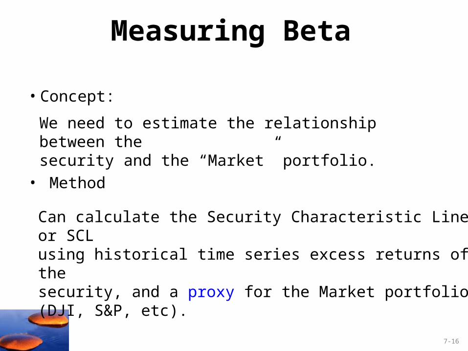
Arbitrage Pricing ModelThe result: For a well diversified portfolio

Rp = βpRS (Excess returns)

(rp – rf) = βp(rS – rf)

and for an individual security

(ri – rf) = βi(rS – rf) + ei

Advantage of the APT over the CAPM:•

• –

No particular role for the “Market Portfolio,” which can’t be measured anyway

Easily extended to multiple systematic factors, for example

=> (ri – rf) = βp,1(r1,i – rf) + βp,2(r2,i – rf) + βp,3(r3,i – rf) + ei

RS is the excess return on a portfolio with a beta of 1 relative to systematic factor “S”

7-33

APT and CAPM Cont.APT employs fewer restrictive assumptions

APT does NOT specify the systematic factors

Chen, Roll and Ross (1986) suggest:

Industrial production

Yield curve

Default spreads

Inflation

7-34

Selected Problems

7-35

Problem 1

– E(rX) =

X =

– E(rY) =

Y =

5% + 0.8(14% – 5%) = 12.2%

14% – 12.2% = 1.8%

5% + 1.5(14% – 5%) = 18.5%

17% – 18.5% = –1.5%

a. CAPM: E(ri) = 5% + β(14% -5%)

CAPM: E(ri) = rf + β(E(rM)-rf)

7-36

Problem 1

b. Which stock?

i. Well diversified:Relevant Risk Measure?

Best Choice?

b. Which stock?

ii. Held alone:Relevant Risk Measure?

Best Choice?β: CAPM Model

Stock X with the positive alpha

Calculate Sharpe ratios

X = 1.8%

Y = -1.5%

7-37

Problem 1

b. (continued) Sharpe Ratios

ii. Held Alone:Sharpe Ratio X =

Sharpe Ratio Y =

Sharpe Ratio Index =

(0.14 – 0.05)/0.36 = 0.25

(0.17 – 0.05)/0.25 = 0.48

(0.14 – 0.05)/0.15 = 0.60

Better

σ

rE(r)Ratio Sharpe f

7-38

Problem 2

E(rP) = rf + [E(rM) – rf]

20% = 5% + (15% – 5%)

= 15/10 = 1.5

7-39

Problem 3

E(rP) = rf + [E(rM) – rf]

E(rp) when double the beta:

If the stock pays a constant dividend in perpetuity, then we know from the original data that the dividend (D) must satisfy the equation for a perpetuity:

Price = Dividend / E(r)

$40 = Dividend / 0.13

At the new discount rate of 19%, the stock would be worth:

$5.20 / 0.19 = $27.37

13% = 7% + β(8%) or β = 0.75

E(rP) = 7% + 1.5(8%) or E(rP) = 19%

so the Dividend = $40 x 0.13 = $5.20

7-40

Problem 4

a.

a.

b.

•

False. = 0 implies E(r) = rf , not zero.

Depends on what one means by ‘volatility.’ If one means the then this statement is false. Investors require a risk premium for bearing systematic (i.e., market or undiversifiable) risk.

False. You should invest 0.75 of your portfolio in the market portfolio, which has β = 1, and the remainder in T-bills. Then:

P = (0.75 x 1) + (0.25 x 0) = 0.75

7-41

Problems 5 & 6

9.

10.

Not possible. Portfolio A has a higher beta than Portfolio B, but the expected return for Portfolio A is lower.

Possible. Portfolio A's lower expected rate of return can be paired with a higher standard deviation, as long as Portfolio A's beta is lower than that of Portfolio B.

7-42

Problem 7

Calculate Sharpe ratios for both portfolios:

Not possible. The reward-to-variability ratio for Portfolio A is better than that of the market, which is not possible according to the CAPM, since the CAPM predicts that the market portfolio is the portfolio with the highest return per unit of risk.

0.5.12

.10.16Sharpe A

0.33

.24

.10.18SharpeM

σ

rE(r)Ratio Sharpe f

7-43

Problem 8

Need to calculate Sharpe ratios?

Not possible. Portfolio A clearly dominates the market portfolio. It has a lower standard deviation with a higher expected return.

8.

7-44

Problem 9

9.

Given the data, the SML is:

E(r) = 10% + (18% – 10%)

A portfolio with beta of 1.5 should have an expected return of:

E(r) = 10% + 1.5(18% – 10%) = 22%

Not Possible: The expected return for Portfolio A is 16% so that Portfolio A plots below the SML (i.e., has an = –6%), and hence is an overpriced portfolio. This is inconsistent with the CAPM.

7-45

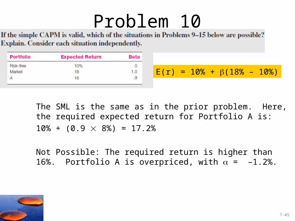
Problem 10

The SML is the same as in the prior problem. Here, the required expected return for Portfolio A is:

10% + (0.9 8%) = 17.2%

Not Possible: The required return is higher than 16%. Portfolio A is overpriced, with = –1.2%.

E(r) = 10% + (18% – 10%)

7-46

Problem 11

Sharpe A =

Sharpe M =

Possible: Portfolio A's ratio of risk premium to standard deviation is less attractive than the market's. This situation is consistent with the CAPM. The market portfolio should provide the highest reward-to-variability ratio.

(16% - 10%) / 22% = .27

(18% - 10%) / 24% = .33

7-47

Problem 12

Since the stock's beta is equal to 1.0, its expected rate of return should be equal to ______________________.

E(r) =

0.18 =

0

011

P

PPD

100

100P9 1 or P1 = $109

)r)β(E(rrP

PPD:mEquilibriu In fMf

0

011

the market return, or 18%

7-48

Problem 13

a.

b.

r1 = 19%; r2 = 16%; 1 = 1.5; 2 = 1.0

We can’t tell which adviser did the better job selecting stocks because we can’t calculate either the alpha or the return per unit of risk.

r1 = 19%; r2 = 16%; 1 = 1.5; 2 = 1.0, rf = 6%; rM = 14%

1 =

2 =

The second adviser did the better job selecting stocks (bigger + alpha)

19% –

16% –

19% – 18% = 1%

16% – 14% = 2%

CAPM: ri = 6% + β(14%-6%)

[6% + 1.5(14% – 6%)] =

[6% + 1.0(14% – 6%)] =

7-50

Problem 14

a.

b.

McKay should borrow funds and invest those funds proportionally in Murray’s existing portfolio (i.e., buy more risky assets on margin). In addition to increased expected return, the alternative portfolio on the capital market line (CML) will also have increased variability (risk), which is caused by the higher proportion of risky assets in the total portfolio.

McKay should substitute low beta stocks for high beta stocks in order to reduce the overall beta of York’s portfolio. Because York does not permit borrowing or lending, McKay cannot reduce risk by selling equities and using the proceeds to buy risk free assets (i.e., by lending part of the portfolio).

7-51

Problem 15

i.

ii.

Since the beta for Portfolio F is zero, the expected return for Portfolio F equals the risk-free rate.

For Portfolio A, the ratio of risk premium to beta is:

The ratio for Portfolio E is:

Create Portfolio P by buying Portfolio E and shorting F in the proportions to give βp = βA = 1, the same beta as A. βp =Wi βi

1 = WE(βE) + (1-WE)(βF);

E(rp) =

WE = 1 / (2/3) or1.5(9) + -0.5(4) = 11.5%,

11.5% - 10% = 1.5%

(10% - 4%)/1 = 6%

(9% - 4%)/(2/3) = 7.5%

WE = 1.5 and WF = (1-WE) = -.5

p,-A =

Buying Portfolio P and shorting A creates an arbitrage opportunity since both have β = 1

7-52

Problem 16

The revised estimate of the expected rate of return of the stock would be the old estimate plus the sum of the unexpected changes in the factors times the sensitivity coefficients, as follows:

Revised estimate = 14% +

E(IP) = 4% & E(IR) = 6%; E(rstock) = 14%

βIP = 1.0 & βIR = 0.4

Actual IP = 5%, so unexpected ΔIP = 1%

Actual IR = 7%, so unexpected ΔIR = 1%

E(rstock) + Δ due to unexpected Δ Factors[(1 1%) + (0.4 1%)] =15.4%