Chapter 7: Balanced flow - Universitetet i Oslo · Chapter 7: Balanced flow 1 ... Global Forecast System-Model . ... - Thermal wind is determined by the horizontal temperature gradient,

GEF 1100 – Klimasystemet

Chapter 7: Balanced flow

1

GEF1100–Autumn 2016 27.09.2016

Prof. Dr. Kirstin Krüger (MetOs, UiO)

1. Motivation

2. Geostrophic motion 2.1 Geostrophic wind 2.2 Synoptic charts 2.3 Balanced flows

3. Thermal wind equation*

4. Subgeostrophic flow: The Ekman layer 5.1 The Ekman layer* 5.2 Surface (friction) wind 5.3 Ageostrophic flow

5. Summary

6. Take home message *With add ons.

Lect

ure

Ou

tlin

e –

Ch

. 7 Ch. 7 – Balanced flow

2

Today‘s weather chart 1. Motivation

www.yr.no 3

Varmfront

Kaldfront

Okklusjon

x

Where does the wind come from in Oslo?

Today‘s 500 hPa (~5 km) weather map

1. Motivation

4 How is the wind blowing? Which forces are acting?

www.wetteronline.de GFS: Global Forecast System-Model

Scale analysis – geostrophic balance -1-

First consider magnitudes of the first 2 terms in momentum eq. for a fluid on a

rotating sphere (Eq. 6-43 𝐷𝐮

𝐷𝑡 + f 𝒛 × 𝒖 +

1

𝜌𝛻𝑝 + 𝛻𝛷 = ℱ) for horizontal

components in a free atmosphere (ℱ=0,𝛻𝛷=0):

•𝐷𝐮

𝐷𝑡 +f 𝒛 × 𝒖 =

𝜕𝑢

𝜕𝑡 + 𝒖 ∙ 𝛻𝒖 + f 𝒛 × 𝒖

• Rossby number R0: - Ratio of acceleration terms (U2/L) to Coriolis term (f U), - R0=U/f L - R0≃0.1 for large-scale flows in atmosphere (R0≃10-3 in ocean, see Chapter 9)

5

2. Geostrophic motion

𝑈

𝑇10−4

𝑈2

𝐿

10−4

fU

10−3

Large-scale flow magnitudes in atmosphere: 𝑢 and 𝑣 ∼ 𝒰, 𝒰∼10 m/s, length scale: L ∼106 m, time scale: 𝒯 ∼105 s, 𝒰 / 𝒯≈ 𝒰2/L ∼10-4 ms-2, f45° ∼ 10-4 s-1

Scale analysis – geostrophic balance -2-

• Coriolis term is left (≙ smallness of R0) together with the pressure gradient term (~10-3):

f 𝒛 × 𝒖 + 1

𝜌𝛻𝑝 = 0 Eq. 7-2 geostrophic balance

• It can be rearranged to (𝒛 × 𝒛 × 𝒖 = −𝒖):

𝒖g=1

𝑓𝜌𝒛 × 𝛻𝑝 Eq. 7-3 geostrophic flow

• In vector component form:

(𝑢g, 𝑣g)= −1

𝑓𝜌

𝜕𝑝

𝜕𝑦,1

𝑓𝜌

𝜕𝑝

𝜕𝑥 Eq. 7-4

6


𝒛 × 𝛻𝑝 =

𝑥 𝑦 𝑧 0 0 1𝜕𝑝

𝜕𝑥

𝜕𝑝

𝜕𝑦

𝜕𝑝

𝜕𝑧

= 𝑥 −𝜕𝑝

𝜕𝑦 + 𝑦

𝜕𝑝

𝜕𝑥

Note: For geostrophic flow the pressure gradient is balanced by the Coriolis term; to be approximately satisfied for flows of small R0.

Geostrophic flow (NH: f>0)


7 Marshall and Plumb (2008)

High: clockwise flow

Low: anticlockwise flow

isobar

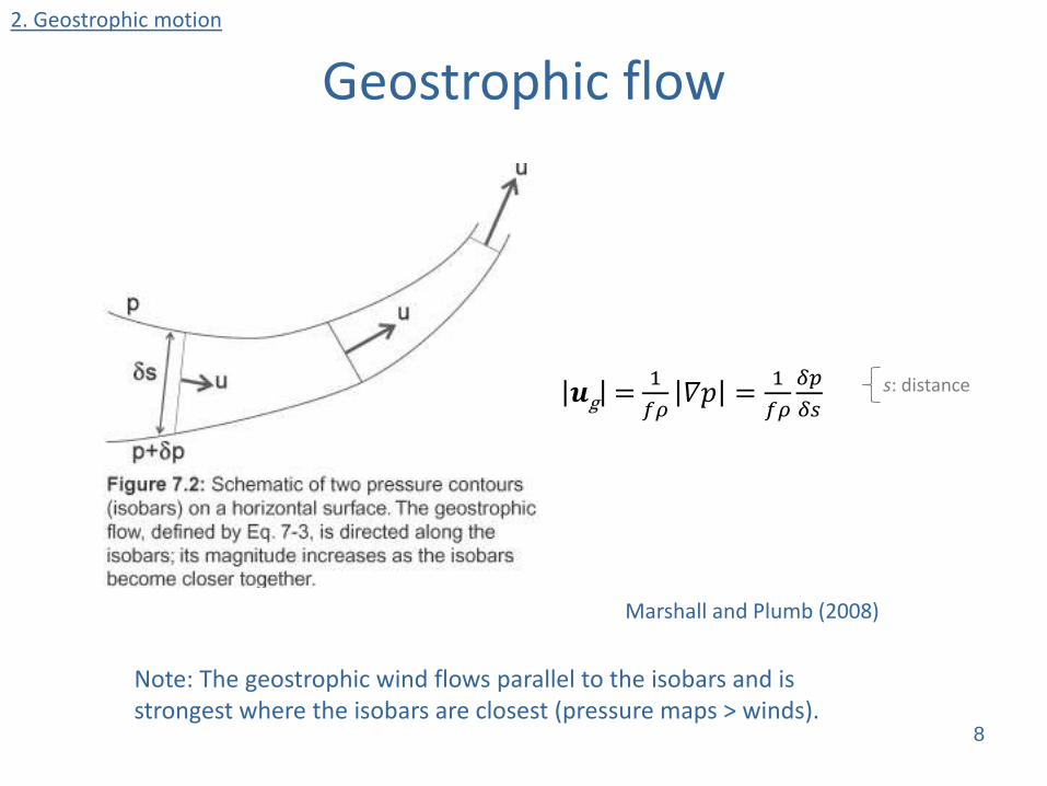
Geostrophic flow 2. Geostrophic motion

8

Marshall and Plumb (2008)

Note: The geostrophic wind flows parallel to the isobars and is strongest where the isobars are closest (pressure maps > winds).

𝒖g = 1

𝑓𝜌𝛻𝑝 =

1

𝑓𝜌

𝛿𝑝

𝛿𝑠 s: distance

L

H

FP

CF

gu

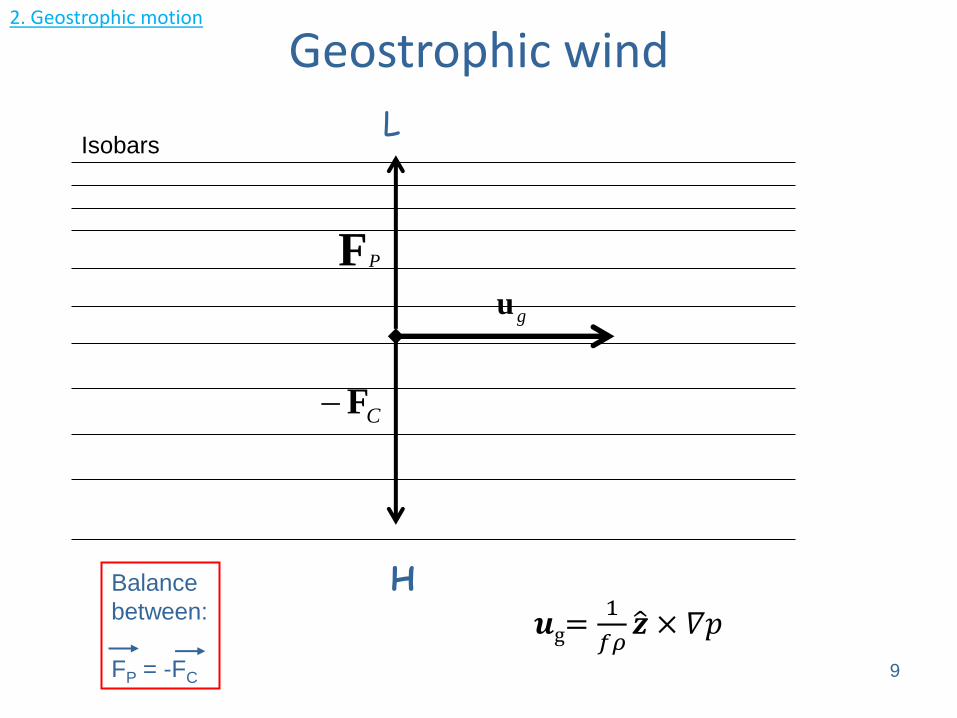
Geostrophic wind

Isobars

Balance

between:

FP = -FC 9


𝒖g=1

𝑓𝜌𝒛 × 𝛻𝑝

L

H

FP

CF

gu

Which rules can be laid down for the geostrophic wind?

1. The wind blows isobars parallel. 2. Seen in direction of the wind, the low pressure lies to the left. 3. The pressure gradient force and the Corolis force balance each other balance motion. The geostrophic wind closely describes the horizontal wind above the boundary layer!

Geostrophic wind

Isobars

Balance

between:

FP = -FC 10


Geostrophic flow – vertical component


Vertical component of geostrophic flow, as defined by Eq. 7-3, is zero. This can not be deduced directly from geostrophic balance (Eq. 7-2). • Consider incompressible fluids (like the ocean):

𝜌 can be neglected, 𝑓~const. for planetary scales, then geostrophic wind components (Eq. 7-4) gives:

𝜕𝑢g

𝜕x+

𝜕𝑣g

𝜕y = 0 Eq. 7-5 ``Horizontal flow is non divergent.’’

Comparison with continuity equation (𝛻 ∙ 𝒖 = 0) => 𝑤g= 0 => 𝜕𝑤g

𝜕z = 0

=> geostrophic flow is horizontal.

• For compressible fluids (like the atmosphere) 𝜌 varies, see next slide.

11

We derive from Eq. 7.3 in pressure coordinates:

𝒖g=g𝑓𝒛𝑝 × 𝛻𝑝z Eq. 7-7

(𝑢g, 𝑣g)= −g𝑓

𝜕𝑧

𝜕𝑦,g𝑓

𝜕𝑧

𝜕𝑥 Eq. 7-8

𝛻𝑝 ∙ 𝒖g =𝜕𝑢

𝜕x+

𝜕𝑣

𝜕y = 0 Eq. 7-9

Geostrophic wind is non-divergent in pressure coordinates, if 𝑓~const. (≤ 1000 km).

Geostrophic wind – pressure coordinates “p”


12


Note: Geopotential height (z) contours are streamlines of the geostrophic flow on pressure surfaces; geostrophic flow streams along z contours (as p contours on height surfaces) (Fig. 7-4).

10 knots

5 knots


13

500 hPa wind and geopotential height (gpm), 12 GMT June 21, 2003 over USA


Note: Geopotential height (zGH≈z; see Chapter 5 Eq. 5.5) contours are streamlines of the geostrophic flow on pressure surfaces; geostrophic flow streams along z contours (as p contours on height surfaces) (Fig. 7-4).

𝒖g=g𝑓𝒛𝑝 × 𝛻𝑝z Eq. 7-7

(𝑢g, 𝑣g)= −g𝑓

𝜕𝑧

𝜕𝑦,g𝑓

𝜕𝑧

𝜕𝑥 Eq. 7-8

Summary: The geostrophic wind ug

• Geostrophic wind: “wind on the turning earth“: Geo (Greek) “Earth“, strophe (Greek) “turning”.

• The friction force and centrifugal forces are negligible.

• Balance between pressure gradient and Coriolis force

→ geostrophic balance

• The geostrophic wind is a horizontal wind.

• It displays a good approximation of the horizontal wind in the free atmosphere; not defined at the equator:

- Assumption: u=ug v=vg

y

p

fug

1

x

p

fvg

1p

f z

1

gu

ρ: density f = 2 Ω sinφ; at equator f = 0 at Pole f is maximum

14





How is the wind blowing? Where are the low and high pressure systems? Which forces are acting?

Quiz




Quiz How is the wind blowing? Where are the low and high pressure systems? Which forces are acting?

H

L

L

17

www.wetteronline.de

Quiz

Tues 27.09.2016 12 UTC, GFS model

H

L

L

H

L

L

How is the wind blowing? Where are the low and high pressure systems? Which forces are acting?

The geostrophic wind ug

Geostrophic wind balance (GWB):

Simultaneous wind and pressure measurements in the open atmosphere show that mostly the GWB is fully achieved.

Advantage: The wind field can be determined directly from the pressure or height fields.

Disadvantage: The horizontal equation of motion becomes purely diagnostic; stationary state.

18


Zonal mean

zonal wind u (m/s)

January average

SPARC climatology

Pre

ssu

re [h

Pa

]

1000

W

W

E

E

E

19


Randel et al 2004

GEF 1100 – Klimasystemet

Chapter 7: Balanced flow

20

GEF1100–Autumn 2016 29.09.2016

Prof. Dr. Kirstin Krüger (MetOs, UiO)

1. Motivation

2. Geostrophic motion 2.1 Geostrophic wind 2.2 Synoptic charts 2.3 Balanced flows

3. Thermal wind equation*

4. Subgeostrophic flow: The Ekman layer 5.1 The Ekman layer* 5.2 Surface (friction) wind 5.3 Ageostrophic flow

5. Summary

6. Take home message *With add ons.

Lect

ure

Ou

tlin

e –

Ch

. 7 Ch. 7 – Balanced flow

21


Rossby number R0 @500hPa, 12 GMT June 21, 2003

Marshall and Plumb (2008) 22

R0 > 0.1

- R0 : Ratio of acceleration term (U/T ≈ U2/L) to Coriolis term (f U) - R0=U/f L - R0≃0.1 for large-scale flows in atmosphere

(Other) Balanced flows

• Geostrophic balance holds, when

small positive R0 (~ 0.1).

Pressure gradient force and Coriolis

force are in balance.

• Gradient wind balance (R0∼1)

Pressure gradient force, Coriolis force and Centrifugal force play a role.

• Cyclostrophic wind balance (R0>1)

Pressure gradient force and Centrifugal force play a role.


23


Gradient wind uG – 2 cases with same Fp

Kraus (2004) 25

L

streamline

streamline

uG

uG

Case 1: sub-geostrophic Case 2: super-geostrophic

Balance between the forces:

Fpressure = -(FCoriolis+ FZ(centrifugal))

Balance between the forces:

Fpressure+ FZ(centrifugal) = -FCoriolis


Cyclostrophic wind

FZ

Balance between: FP = -FZ

- Physically appropriate solutions are orbits around a low pressure centre, that can run both cyclonically (counter clockwise) as well as anticyclonically (clockwise). - The cyclostrophic wind appears in small-scale whirlwinds (dust devils, tornados).

26

L


The thermal wind

ug(z)

ug(z+Δz)

T

Altitude z

Geostrophic wind change with altitude z?

→”Thermal wind” (∆zug)

Applying geostrophic wind equation together with ideal gas law (Eq. 1-1 p=ρRT); insert finite vertical layer ∆z* with average temperature T, leads to: (*∆: finite difference)

27

3. Thermal wind equation

z

Δz

𝒖g: geostrophic wind vector, T: temperature 𝜌: density p: pressure; R: gas constant for dry air, g: gravity acceleration, 𝑓: Coriolis parameter, z: geometric height, 𝒛 : unit vector in z−direction

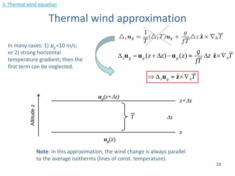
Thermal wind approximation

ug(z)

ug(z+Δz)

T

Altitude z

z

Δz

z+Δz

Thgz zu ˆ

In many cases: 1) ug <10 m/s; or 2) strong horizontal temperature gradient; then the first term can be neglected.

TzTf

gzzz hgggz zuuu ˆ)()(

28

Note: In this approximation, the wind change is always parallel to the average isotherms (lines of const. temperature).


z

y

Which rules can I deduce from the thermal wind approximation?

- The geostr. wind change with height is parallel to the mean isotherms, - whereby the colder air remains to the left on the NH, - geostrophic left rotation with increasing height for cold air advection, - geostrophic right rotation with increasing height for warm air advection.


x

29

∆z ug ∆z ug

ug (z+∆z ) ug (z+∆z )

ug (z) ug (z)

cold

cold air advection warm

warm air advection

cold


warm

y

Which rules can I deduce from the thermal wind approximation, if ug<10 m/s ?

- The geostr. wind change with height is parallel to the mean isotherms, - whereby the colder air remains to the left on the NH, - geostrophic left rotation with increasing height for cold air advection, - geostrophic right rotation with increasing height for warm air advection.


x

30

∆z ug ∆z ug

ug (z+∆z ) ug (z+∆z )

ug (z) ug (z)

cold

cold air advection warm

warm air advection

cold


isotherm

Thermal wind:

Compare: - Thermal wind is determined by the horizontal temperature gradient, - geostrophic wind through the horizontal pressure gradient.

Geostrophic wind:

x

p

fvg

1

x

T

f

agzvzzv

z

v

y

T

f

agzuzzu

z

u

gg

g

gg

g

)()(

)()(

y

p

fug

1

31

3. Thermal wind equation - Summary

𝜕𝒖g

𝜕𝑧=

𝑎g𝑓𝒛 × 𝛻𝑇 Eq. 7-18

𝒖g=1

𝑓𝜌𝒛 × 𝛻𝑝 Eq. 7-3

𝒖g=𝑔

𝑓 𝒛𝑝 × 𝛻𝑝 𝑧 Eq. 7-7

𝑎: Thermal expansion coefficient (Ch. 4) g: Gravity acceleration

Thermal wind – examples



W W

C W C

W W

90N 90S

33



x x Oslo

Temperature (°C) @500hPa, 12 GMT June 21, 2003

cold air

warm air

34



C W

W

70N 20N

Westerly wind

Easterly wind

Warm

Cold

E



Stratospheric polar vortex

Sub-geostrophic flow: The Ekman layer

36

𝑓𝒛 × 𝒖 +1

𝜌𝛻𝑝 = ℱ Eq. 7-25

• Large scale flow in free atmosphere and ocean is close to geostrophic and thermal wind balance.

• Boundary layers have large departures from geostrophy due to friction forces.

Ekman layer: - Friction acceleration ℱ becomes important,

- roughness of surface generates turbulence in the first ~1 km of the atmosphere,

- wind generates turbulence at the ocean surface down to first 100 meters.

Sub-geostrophic flow: R0 small, ℱ exists, then horizontal component of momentum (geostrophic) balance (Eq. 7-2) can be written as:

4. Sub-geostrophic flow

Surface (friction) wind

37


𝑓𝒛 × 𝒖 +1

𝜌𝛻𝑝 = ℱ Eq. 7-25

4. Subgeostrophic flow

ℱ − 𝑓𝒛 × 𝒖 and

1. Start with u 2. Coriolis force per unit mass must be to the right of u 3. Frictional force per unit mass acts as a drag and must be opposite to u. 4. Sum of the two forces (dashed arrow) must be balanced by the pressure gradient force per unit mass 5. Pressure gradient is not normal to the wind vector or the wind is no longer directed along the isobars, however the low pressure system is still on the left side but with a deflection.

=> The flow is sub-geostrophic (less than geostrophic); ageostrophic component directed from high to low.

The Ekman spiral – theory

Roedel, 1987

uh

ug

The Ekman spiral was first calculated for the oceanic friction layer by the Swedish oceanographer in 1905. In 1906, a possible application in Meteorology was developed.

u0

38


𝑓𝑧 × 𝒖 +1

𝜌𝛻𝑝 = ℱ Eq. 7-25

ℱ = 𝜇 𝜕2𝒖/𝜕𝑧2

𝜇: constant eddy viscosity

Ekman spiral: simplified theoretical calculation

Wind measurement in the boundary layer

Kraus, 2004 The “Leipzig wind profile”

39

uh

ug

m


The ageostrophic flow uag

The ageostrophic flow is the difference between the geostrophic

flow (ug) and the horizontal flow (uh):

uh = ug+ uag Eq. 7-26

𝑓𝒛 × 𝒖ag = ℱ Eq. 7-27

The ageostrophic component is always directed to the right of ℱ

in the NH.

40


ug

uh

uag

H L


Surface (friction) wind


41

Low pressure (NH): - anticlockwise flow - often called “cyclone”

High pressure (NH): - clockwise flow - often called “anticyclone”

Note: At the surface the wind is blowing from the high to the low pressure system.

Today‘s weather chart Quiz

www.yr.no 42

Varmfront

Kaldfront

Okklusjon

What is the wind direction and approximately wind strength in Oslo? a) Weak northeasterly. b) Fresh southwesterly. c) Storm from the west. d) Storm from the east.

x x Oslo

Beaufort

wind scale

44

«Sir Francis Beaufort var en irsk hydrograf og offiser i den britiske marinen. I 1806 satte han navn på vindens styrke. Denne skalaen brukes i dag i all vanlig værvarsling.»

http://om.yr.no/forklaring/symbol/vind/

Vertical motion induced by Ekman layers

• Ageostrophic flow is horizontally divergent.

• Convergence/divergence drives vertical motions.

• In pressure coordinates, if f is const., the continuity equation (Eq. 6-12) becomes:

𝛻𝑝 ∙ 𝒖𝑎𝑔 + 𝜕𝑤

𝜕𝑝 = 0

• Low: convergent flow

• High: divergent flow

• Continuity equation requires vertical motions:

- “Ekman pumping“ > ascent

- “Ekman suction” > descent



45

Characteristics of horizontal wind

Combination of horizontal and vertical vergences

46


47


Surface pressure (hPa) and wind (kn), 12 GMT June 21, 2003, USA

10 knots

5 knots


Tomorrow’s surface pressure (hPa) map


48

www.met.fu-berlin.de

30. Sept

12 UTC,

DWD ICON

model

x Oslo x


See also chapter 8.


50

Summary of chapters 6 and 7

𝑓𝜕𝒖

𝜕𝑧= 𝑎𝑔 𝒛 × 𝛻𝑇

5. Summary

• Balanced flows for horizontal fluids (atmosphere and ocean).

• Balanced horizontal winds:

– Geostrophic wind balance good approximation for the observed wind in the free troposphere.

– Gradient wind balance and cyclostrophic wind balance occur with higher Rossby number.

– Surface wind (subgeostrophic flow) balance occurs within the Ekman layer.

• Thermal wind is good approximation for the geostrophic wind change with height z.

Take home message

51

Zonal mean temperature (°C)

Pre

ssu

re [h

Pa

]

Which winds play a role in the below shown climatology?

Zonal mean zonal wind (m/s)

52

Quiz

Documents

Chapter 7: Balanced flow - Universitetet i Oslo · Chapter 7: Balanced flow 1 ... Global Forecast System-Model . ... - Thermal wind is determined by the horizontal temperature gradient,