Embed Size (px)
Citation preview
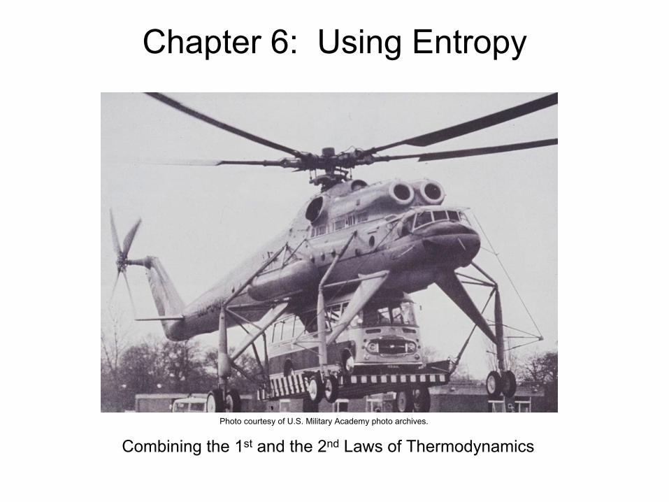
Chapter 6: Using Entropy
Combining the 1st and the 2nd Laws of Thermodynamics
Photo courtesy of U.S. Military Academy photo archives.

ENGINEERING CONTEXT
Up to this point, our study of the second law has been concerned primarily with what it says about systems undergoing thermodynamic cycles. In this chapter means are introduced for analyzing systems from the second law perspective as they undergo processes that are not necessarily cycles. The property entropyplays a prominent part in these considerations.
The objective of the present chapter is to introduce entropy and show its use for thermodynamic analysis.
The word energy is so much a part of the language that you were undoubtedly familiar with the term before encountering it in early science courses. This familiarity probably facilitated the study of energy in these courses and in the current course in engineering thermodynamics. In the present chapter you will see that the analysis of systems from a second law perspective is conveniently accomplished in terms of the property entropy. Energy and entropy are both abstract concepts. However, unlike energy, the word entropy is seldom heard in everyday conversation, and you may never have dealt with it quantitatively before. Energy and entropy play important roles in the remaining chapters of this book.

Introducing Entropy
Corrollary of Second Law is introduced:
Clasius Inequality
Expands last chapter treatment of Two heat reservoirsto arbitrary number of heat reservoirs from which systemreceives energy by heat transfer or rejects energy by heat transfer
Provides basis for two concepts of second law for analyzingclosed and open systems:
1) Entropy as a Property2) Entropy Balance
Represents heat transfer at local system boundary location, b, at temperature T. Heat transfer may be positive (IN) or negative (OUT)
Clasius Inequality
Qδ
0b
QTδ ≤ ∫For any thermodynamic cycle
For any number of reservoirs:
T must be absolute temperature (Kelvin or Rankine)T always positive. Can NOT be negative (Celsius or Farenheit)
∫ Indicates integration over all processes and all parts of boundary

Clasius Inequality
0b
QTδ ≤ ∫
Inequality has same meaning as with Kelvin-Planck:
Equality applies when no INTERNAL IRREVERSIBILITES are present
Inequality applies when INTERNAL IRREVERSIBILITES are present
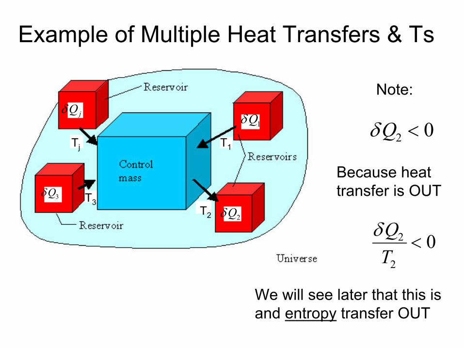
Example of Multiple Heat Transfers & Ts
1Qδ
2Qδ3Qδ
jQδ
T1Tj
T3T2
2 0Qδ <
Note:
2
2
0QTδ
<
Because heat transfer is OUT
We will see later that this is and entropy transfer OUT
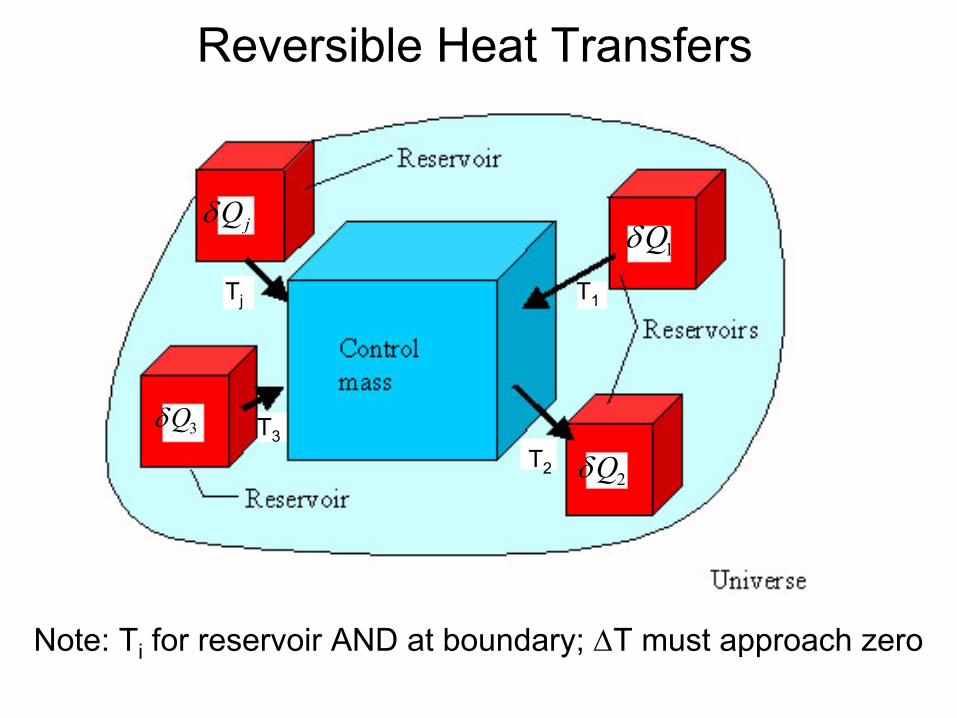
Reversible Heat Transfers
1Qδ
2Qδ3Qδ
jQδ
T1Tj
T3T2
Note: Ti for reservoir AND at boundary; ∆T must approach zero

Developing Clasius Inequality
“Proof” provided in text

cycleb
QTδ σ = − ∫
0b
QTδ ≤ ∫
0cycleb
QTδ σ + = ∫
Alternate Statements of Clasius Inequality
0generatedb
QTδ σ + = ∫

cycleb
QTδ σ = − ∫
0 no irreversibilities present within the system0 irreversibilities present within the system0 impossible
cycle
cycle
cycle
σ
σ
σ
=
>
<
Alternate Statements of Clasius Inequality
0generatedb
QTδ σ + = ∫
Unlike mass and energy, which are conserved in every process, entropy in the presence of
irreversibilities, is always produced.

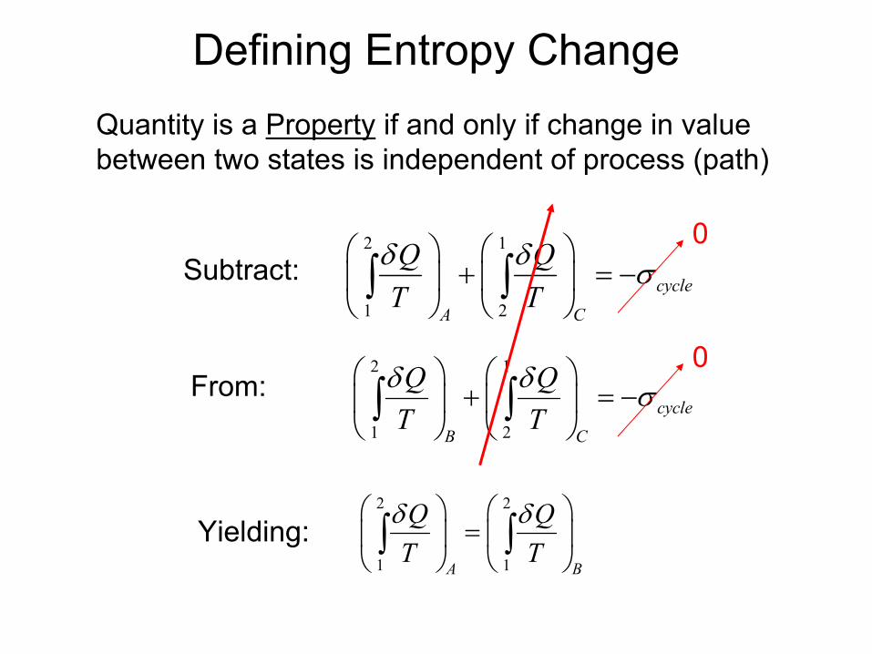
Defining Entropy Change
Quantity is a Property if and only if change in valuebetween two states is independent of process (path)
Will now show that the quantity is a PropertyReversible
QTδ
∫
Meaning: For a REVERSIBLE process, the integral of the heat transfer divided by the local absolute temperature doesNOT depend on the process
This integral is therefore a PROPERTY
We will give this property the name “ENTROPY”

Defining Entropy Change
1
2C
B A
2 1
1 2cycle
A C
Q QT Tδ δ σ
+ = −
∫ ∫
2 1
1 2cycle
B C
Q QT Tδ δ σ
+ = −
∫ ∫
Cycle A-C:
Cycle B-C:
0
0
Quantity is a Property if and only if change in valuebetween two states is independent of process (path)
Processes A, B and C are INTERNALLY REVERSIBLE:
0cycle generatedσ σ= =
Defining Entropy Change
2 2
1 1A B
Q QT Tδ δ
= ∫ ∫
2 1
1 2cycle
A C
Q QT Tδ δ σ
+ = −
∫ ∫
2 1
1 2cycle
B C
Q QT Tδ δ σ
+ = −
∫ ∫
Subtract:
From:
0
0
Quantity is a Property if and only if change in valuebetween two states is independent of process (path)
Yielding:
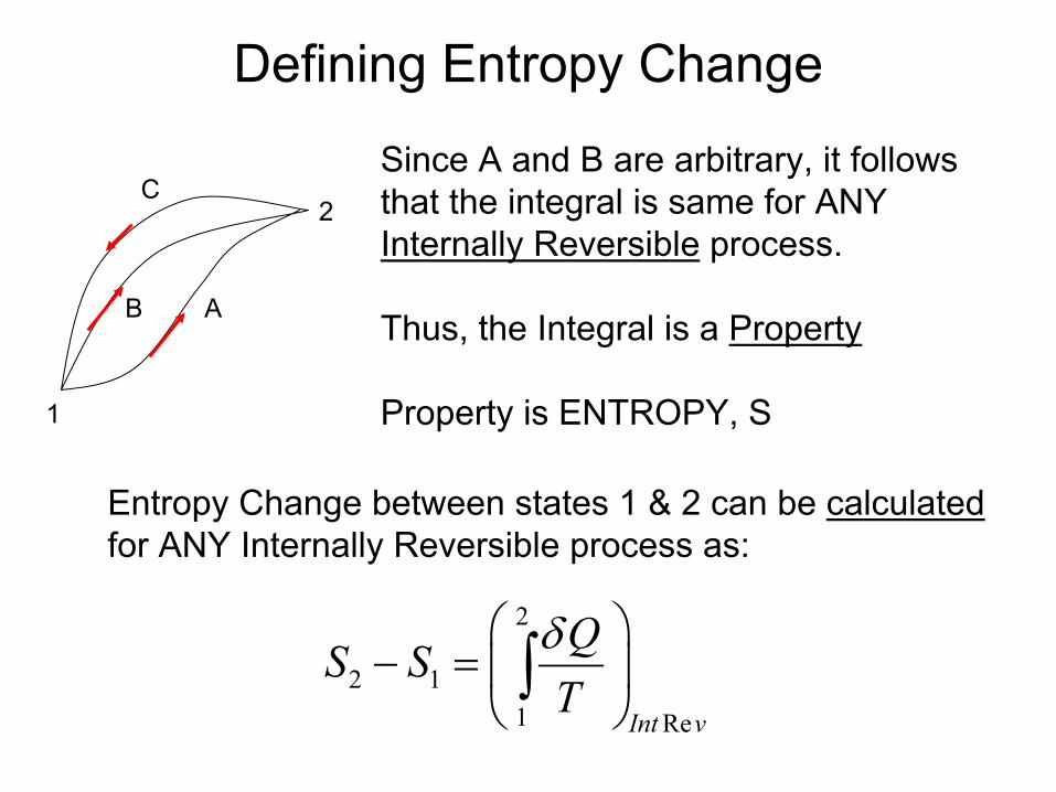
Defining Entropy Change
1
2C
B A
Since A and B are arbitrary, it follows that the integral is same for ANYInternally Reversible process.
Thus, the Integral is a Property
Property is ENTROPY, S
Entropy Change between states 1 & 2 can be calculated for ANY Internally Reversible process as:
2
2 11 ReInt v
QS STδ
− = ∫
Entropy Change
ReInt v
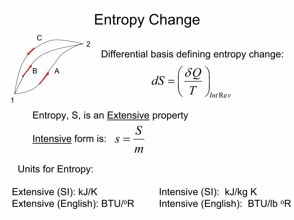
QdSTδ =
1
2C
B A
Differential basis defining entropy change:
Entropy, S, is an Extensive property
Intensive form is: Ssm
=
Units for Entropy:
Extensive (SI): kJ/K Intensive (SI): kJ/kg KExtensive (English): BTU/oR Intensive (English): BTU/lb oR

Defining Entropy Change
1
2C
B A
Important Note:
Entropy change between states 1 & 2 is SAME whether process between 1 & 2 is REVERSIBLE or IRREVERSIBLE.Just can’t calculate change for IRREVERSIBLE processes.
Entropy change between states 1 & 2 can be calculatedfor ANY Internally Reversible process as:
2
2 11 ReInt v
QS STδ
− = ∫
Once calculated, Entropy difference is known

Recognize that Entropy is still an abstract concept for you
Like enthalpy we defined earlier, to gain appreciation for Entropy, need to understand:
HOW to use it
and
WHAT it is used for

Retrieving Entropy Data
Chapter 3: Means for retrieving property data fromTables, graphs, equations (and software)
Emphasis on properties: P, v, T, h
Which are required for:
1st Law (energy conservation) and mass conservation
For application of 2nd Law, entropy values usually needed
Thus, we need to understand how to retrieve entropy data

Entropy Reference Value?Similarity to Energy with regard to absolute values of Entropy
In most cases, absolute values not important- Only difference in Entropy between states is important
1
2C
B A
S1 = ?
S2 = ?
Sref,1
Sref,2
Re
y
y xx Int v
QS STδ
= + ∫
Sx is reference value

Finding Entropy DataFor Water and Refrigerants:
Using Tables A-2 to A-18
and Tables A-2E to A-18E
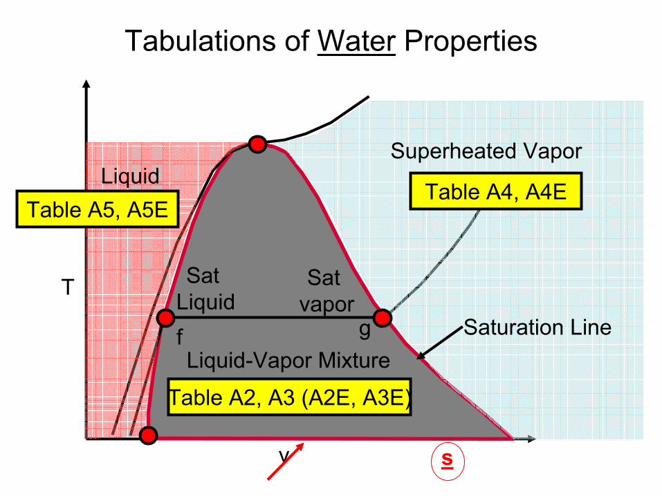
Tabulations of Water Properties
T
v
Liquid
Liquid-Vapor Mixture
Superheated Vapor
Saturation Line
Table A5, A5E
Table A2, A3 (A2E, A3E)
Table A4, A4E
f g
Sat Liquid
Sat vapor
s
Two Saturated Tables for Each
One for Saturated Temperature
One for Saturated Pressure
Sometimes we know T, sometimes P

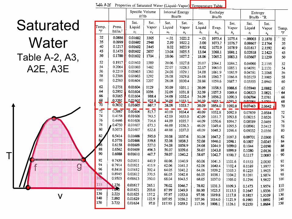
Saturated Water
Table A-2, A3, A2E, A3E
T
s
f g

Computing Entropy Value Under Dome
1
(1 )
liquid vapor
liq vap
liq f vap g
vap
liq
f g
S S S
S SSsm m mm s m s
sm mm
xm
mx
ms x s xs
= +
= = +
= +
=
= −
∴ = − +
It is not enough to know T, P in order to establish state under dome
Need T or P, and one other property
(x= Quality)
T
s
f g
( )f g f f fgs s x s s s x s= + − = + i
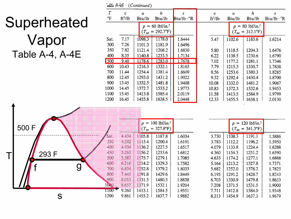
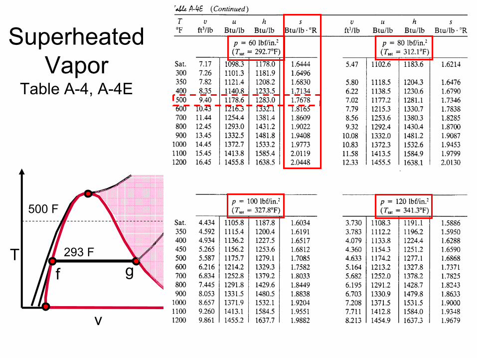
Superheated Vapor
Table A-4, A-4E
T
s
f g293 F
500 F

Compressed or Sub-cooled
LiquidTable A-5, A-5E
Note:sub-cooled tables are sparse because it is accurate to use incompressible liquid model
T
v
f g

Text Examples
Problem solving using property diagrams is important
Two commonly used property diagrams are:
Temperature- Entropy (T-s diagram)
Enthalpy- Entropy (Mollier diagram)

Graphical Entropy Data
Temperature-Entropy Diagram Enthalpy-Entropy (Mollier) Diagram

Note general features
See Figs A-7 & A-7E for water
Temperature-Entropy Diagram
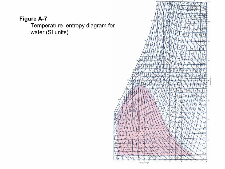
Figure A-7Temperature–entropy diagram for water (SI units)
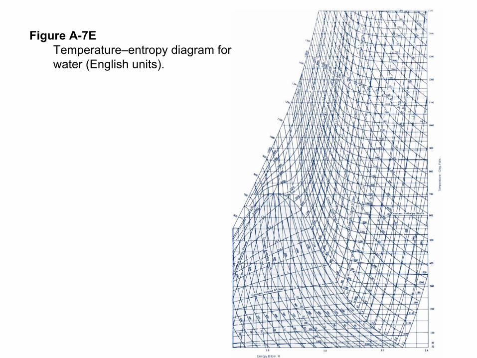
Figure A-7ETemperature–entropy diagram for water (English units).
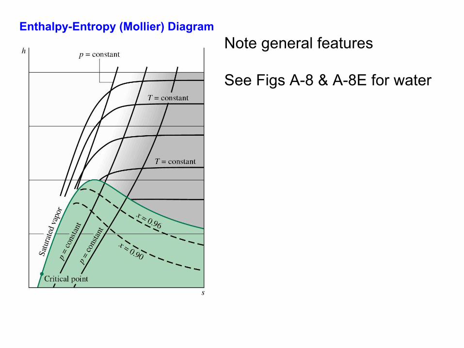
Enthalpy-Entropy (Mollier) DiagramNote general features
See Figs A-8 & A-8E for water
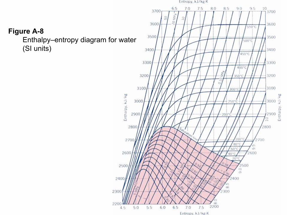
Figure A-8Enthalpy–entropy diagram for water (SI units)
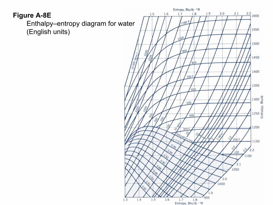
Figure A-8EEnthalpy–entropy diagram for water (English units)

Examples as per text here

Using T dS EquationsAlthough entropy changes can be determined from:
2
2 11 ReInt v
QS STδ
− = ∫
This requires knowledge of how heat transfer and Q vary during a process.
In practice, entropy changes calculated from changes in other properties.
Let’s see how….
Using T dS Equations
Note that T dS equations are also important with respect to:
1) Deriving other important properties
2) Constructing property tables (Chapter 11)

Simple Compressible Substance
( ) ( )Re ReInt v Int vQ dU Wδ δ= +
( ) ReInt vW PdVδ =
TdS dU PdV= +
( ) ReInt vQ TdSδ =
Energy balance in differential form: IN = STORED + OUT
Neglecting KE and PE
First TdS Equation:
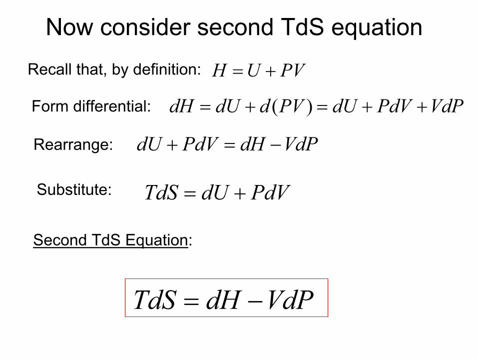
Now consider second TdS equation
TdS dU PdV= +
H U PV= +
( )dH dU d PV dU PdV VdP= + = + +
Second TdS Equation:
Recall that, by definition:
Form differential:
dU PdV dH VdP+ = −Rearrange:
Substitute:
TdS dH VdP= −
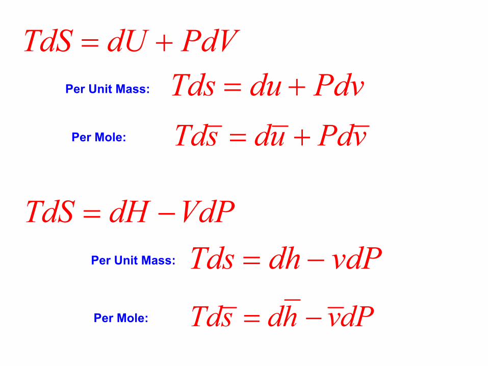
TdS dH VdP= −Per Unit Mass: Tds dh vdP= −
Per Mole: Tds dh vdP= −
TdS dU PdV= +Tds du Pdv= +Per Unit Mass:
Per Mole: Tds du Pdv= +

Although internally reversible processes used to derive these equations, they apply generally- do not require reversible processes.
Since all terms are properties, applies to irreversibleand reversible processes (path-independent)
Change in Entropy is independent of details of process

Text Example
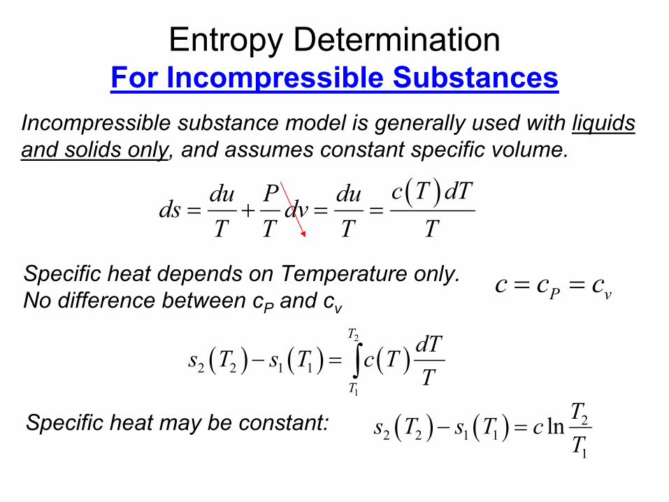
Entropy Determination For Incompressible Substances
P vc c c= =
Incompressible substance model is generally used with liquids and solids only, and assumes constant specific volume.
( ) ( ) ( )2
1
2 2 1 1
T
T
dTs T s T c TT
− = ∫
( )c T dTdu P duds dvT T T T
= + = =
Specific heat depends on Temperature only. No difference between cP and cv
Specific heat may be constant: ( ) ( ) 22 2 1 1
1
ln Ts T s T cT
− =
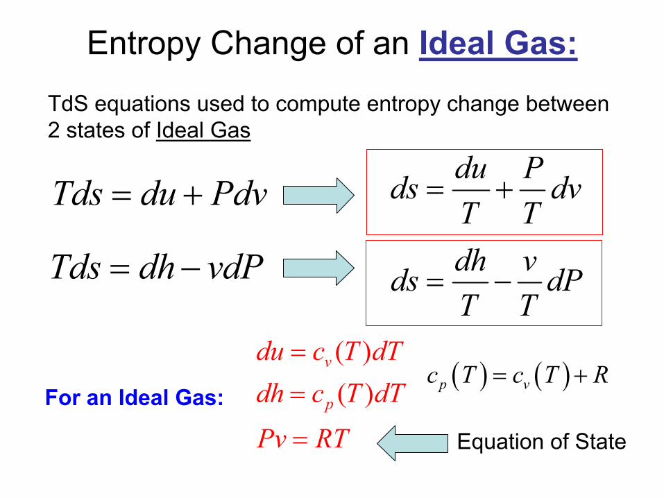
Entropy Change of an Ideal Gas:TdS equations used to compute entropy change between 2 states of Ideal Gas
For an Ideal Gas:
Equation of State
Tds dh vdP= −
Tds du Pdv= +
dh vds dPT T
= −
du Pds dvT T
= +
( ) ( )p vc T c T R= +( )( )
v
p
du c T dTdh c T dT
Pv RT
==
=

Substitute Ideal Gas Relations into TdS equations:
( )( )
v
p
du c T dTdh c T dT
Pv RT
==
=dh vds dPT T
= −
du Pds dvT T
= +
( )pdT dPds c T RT P
= −
( )vdT dvds c T RT v
= + ( ),s s T v=
( ),s s T P=

Can integrate these equations:
( )vdT dvds c T RT v
= +
( )pdT dPds c T RT P
= −
( ) ( ) ( )2
1
22 2 2 1 1 1
1
, , lnT
vT
dT vs T v s T v c T RT v
− = +
∫
( ) ( ) ( )2
1
22 2 2 1 1 1
1
, , lnT
PT
dT Ps T P s T P c T RT P
− = −
∫

Using Ideal Gas Tables:
Thus, in the equation:Where is an arbitrary reference temperatureT ′
( ) ( )Tpo
T
c Ts T dT
T′
= ∫Where
Let’s define a new variable: ( )os T
( ) ( ) ( )2
1
22 2 2 1 1 1
1
, , lnT
PT
dT Ps T P s T P c T RT P
− = −
∫
( ) ( ) ( ) ( ) ( )2 2 1
1
2 1
T T To o
P P PT T T
dT dT dTc T c T c T s T s TT T T′ ′
= − = −∫ ∫ ∫

This integral can be tabulated (Ideal Gas Tables)Tables A-22, A22E:
( ) ( ) ( )2
1
0 02 1
Tp
T
c Ts T s T dT
T− = ∫ (kJ/kg K or BTU/lb oR)
( ) ( ) ( ) ( ) 22 2 2 1 1 1 2 1
1
, , lno o Ps T P s T P s T s T RP
− = − −
( ) ( ) ( )2
1
22 2 2 1 1 1
1
, , lnT
PT
dT Ps T P s T P c T RT P
− = −
∫
Becomes:
Where:
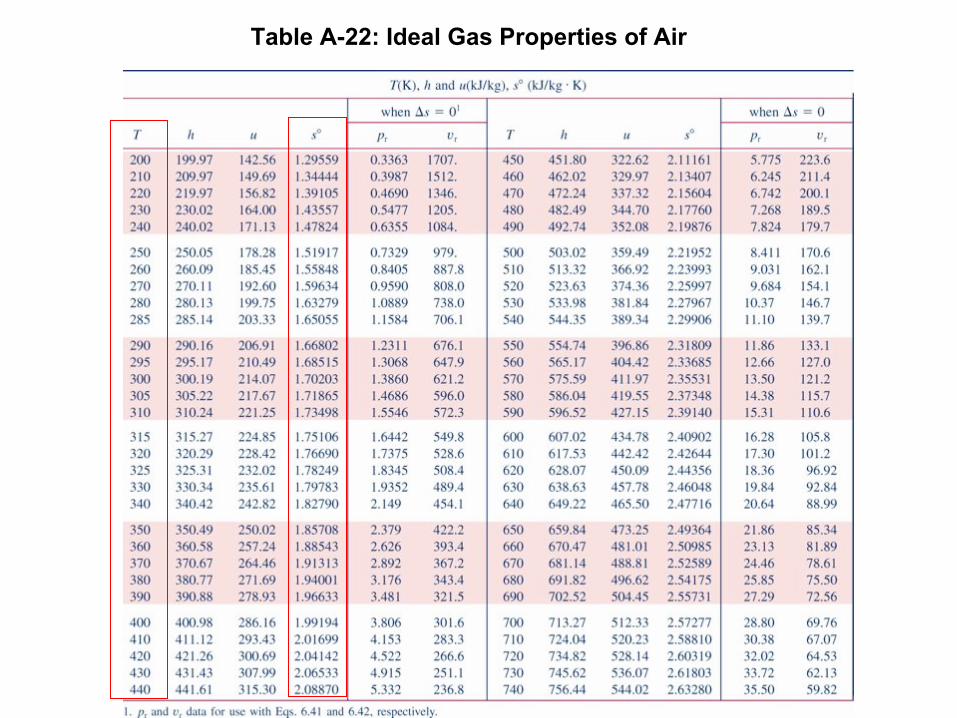
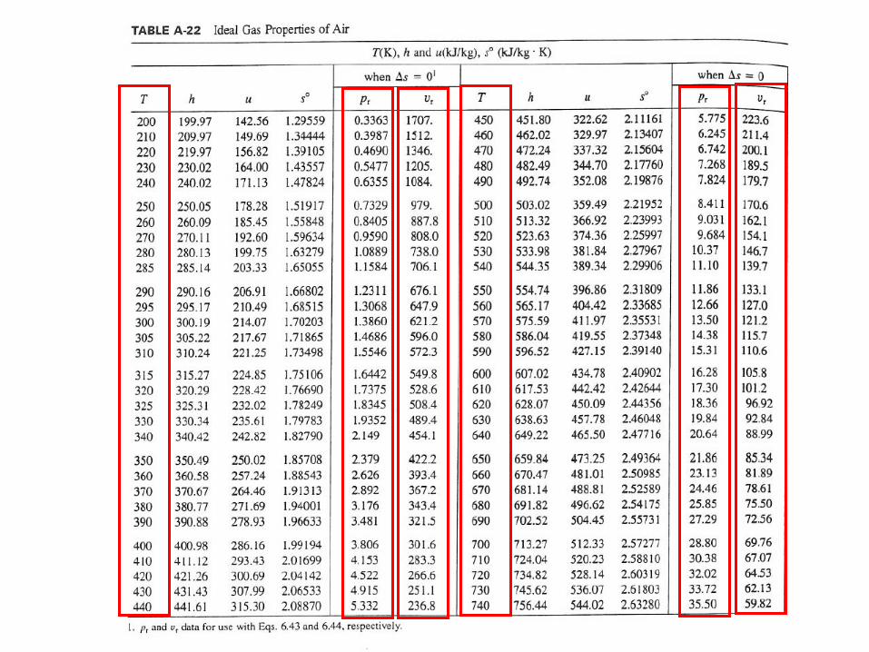
Table A-22: Ideal Gas Properties of Air
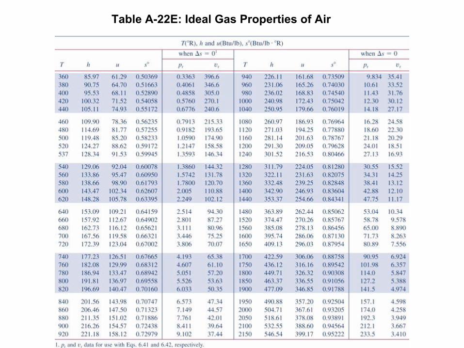
Table A-22E: Ideal Gas Properties of Air

Using Ideal Gas Tables:
Similar approach for per mole basis
( ) ( ) 22 2 1 1 2 1
1
, , ( ) ( ) ln Ps T P s T P s T s T RP
− = − −
This integral can be tabulated (Ideal Gas Tables)Tables A-23, A23E:
What if we have T and v information, rather than T and P?
( ) ( ) ( )2
1
22 2 2 1 1 1
1
, , lnT
vT
dT vs T v s T v c T RT v
− = +
∫
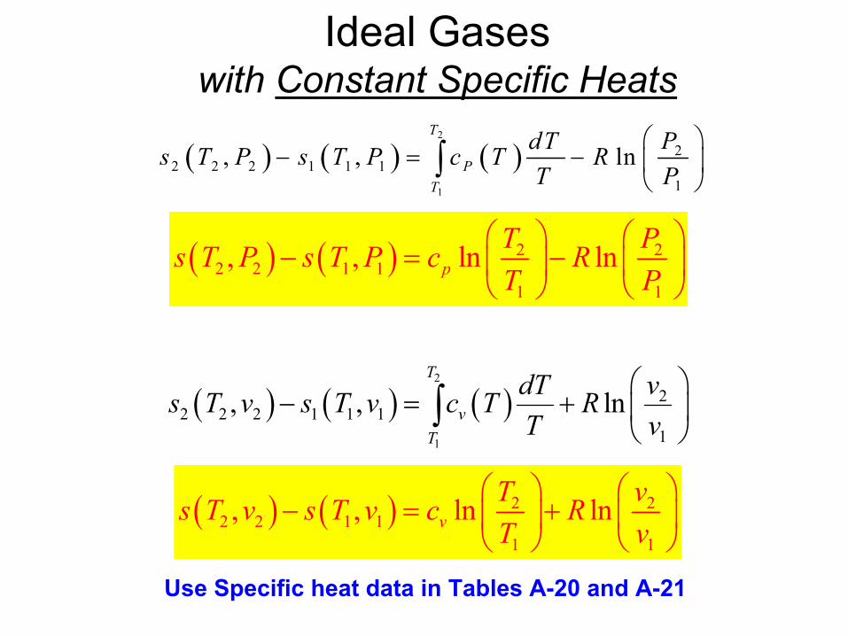
Ideal Gaseswith Constant Specific Heats
( ) ( ) 2 22 2 1 1
1 1
, , ln lnpT Ps T P s T P c RT P
− = −
( ) ( ) 2 22 2 1 1
1 1
, , ln lnvT vs T v s T v c RT v
− = +
( ) ( ) ( )2
1
22 2 2 1 1 1
1
, , lnT
vT
dT vs T v s T v c T RT v
− = +
∫
( ) ( ) ( )2
1
22 2 2 1 1 1
1
, , lnT
PT
dT Ps T P s T P c T RT P
− = −
∫
Use Specific heat data in Tables A-20 and A-21

Table A-20: Ideal Gas Specific Heats of Some Common Gases (kJ/kg · K)

Entropy Change for Closed Systems Internally Reversible Processes
ReInt v
QdSTδ =
For Internally Reversible Processes,Entropy change can be calculated from:
This links heat transfer and entropy transfer
Note that for Closed, Internally Reversible system:
Entropy INCREASES when heat transfer INEntropy DECREASES when heat transfer OUTEntropy DOES NOT CHANGE when no heat transfer occurs
Entropy transfer ACCOMPANIES heat transfer

Entropy Change for Closed Systems Internally Reversible Processes
Q & Entropy IN Q & Entropy OUTQ=0∆S=0
Process where Q = 0 is: ADIABATIC (Insulated)
For process that is ADIABATIC AND REVERSIBLE,The ENTROPY DOES NOT change.
A constant Entropy process is called ISENTROPIC
Thus, an ADIABATIC AND REVERSIBLE processis an ISENTROPIC process
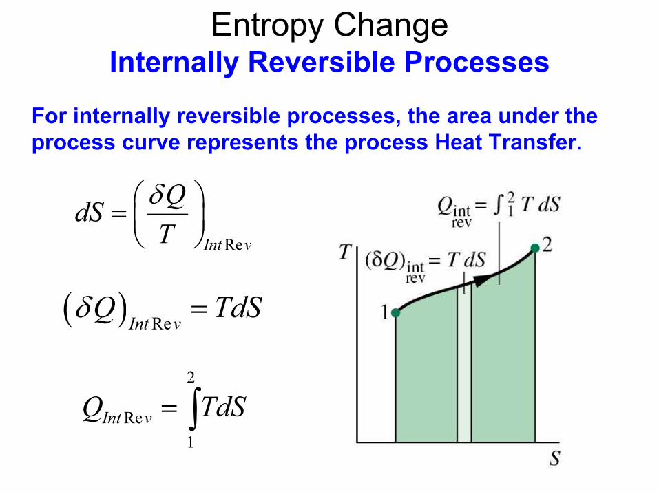
Entropy Change Internally Reversible Processes
( ) ReInt vQ TdSδ =
ReInt v
QdSTδ =
For internally reversible processes, the area under the process curve represents the process Heat Transfer.
2
Re1
Int vQ TdS= ∫

1) Heat transfer is entire area under T-S diagram
2) Temperature must be absolutescale (Kelvin or Rankine), >0
3) Not valid for IRREVERSIBLEprocesses. Then area is NOTequal to heat transfer
Entropy Change Internally Reversible Processes
QdSTδ
≥
Q TdSδ ≤QdSTδ
≥

Entropy Change Internally Reversible Processes
Internally reversible processes are idealizations, but are found in all Carnot cycles.
Carnot cycles on the T-S diagram. The diagram on the left represents a power cycle, and on the right, a refrigeration/heat pump cycle.

Internally reversible processes are idealizations, but are found in all Carnot cycles.
Areas (+ or -) is magnitude of work: W = QIN –QOUT
1cycle C
IN H
W TQ T
η = = −
Power Cycle Refrigeration Cycle
Note how “separation” of TH and TC related to more work

Example in text
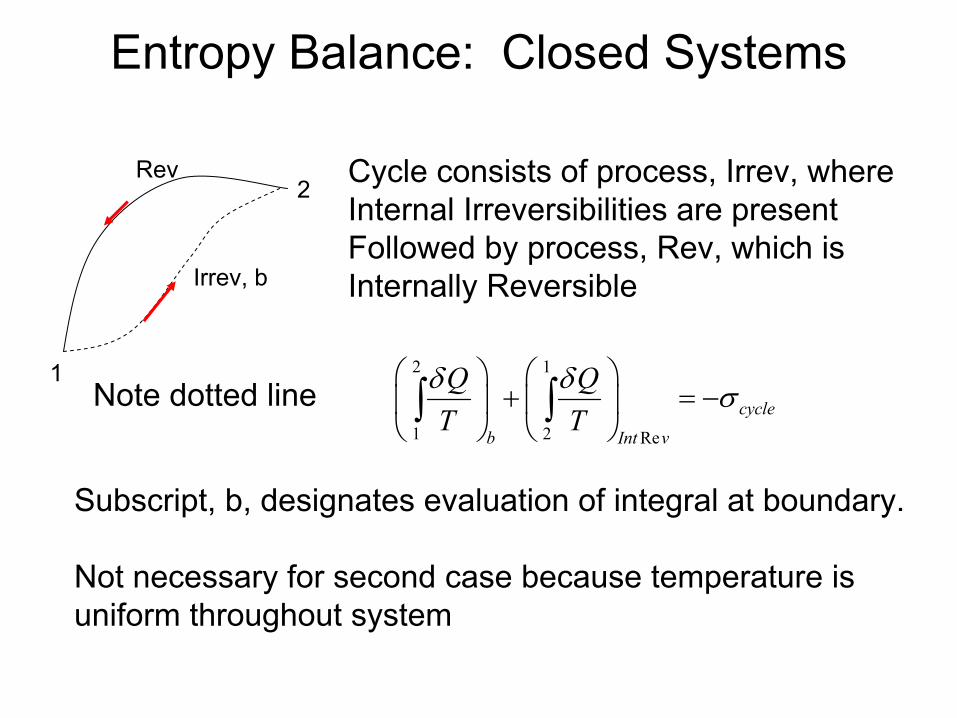
Entropy Balance: Closed Systems
1
2Rev
Irrev, b
Cycle consists of process, Irrev, where Internal Irreversibilities are presentFollowed by process, Rev, which isInternally Reversible
2 1
1 2 Re
cycle
b Int v
Q QT Tδ δ σ
+ = −
∫ ∫
Subscript, b, designates evaluation of integral at boundary.
Not necessary for second case because temperature isuniform throughout system
Note dotted line

Entropy Balance: Closed Systems
2 1
1 2 Re
cycle
b Int v
Q QT Tδ δ σ σ
+ = − = −
∫ ∫
1
1 22 ReInt v
QS STδ
− = ∫
( )2
1 21 b
Q S STδ σ
+ − = −
∫
1
2Rev
Irrev
Cycle consists of process, Irrev, where Internal Irreversibilities are presentFollowed by process, Rev, which isInternally Reversible
Where:
( )2
2 11 b
QS STδ σ
− = +
∫
Entropy Change = Entropy + EntropyTransfer Production

Entropy Balance: Closed Systems
Total entropy change associated with heat transfer (+ or -)AND entropy generated by IRREVERSIBILITIES (ALWAYS + or 0)
Can INCREASE or DECREASE entropy by heat transferIRREVERSIBILITY will ALWAYS INCREASE entropy
ZERO entropy generated for a REVERSIBLE process
( )2
2 11 b
QS STδ σ
− = +
∫
Entropy Change = Entropy + EntropyTransfer Production

Entropy Balance: Closed Systems2
2 11 b
QS STδ σ − = + ∫
Entropy Change
Entropy Transfer
Entropy Production
Since σ measures the effect of irreversibilitiespresent within the system during a process,
its value depends on the nature of the process, and thus is NOT a property
2
2 11 b
QS STδ − ≥ ∫

Some Examples
Reversible, Adiabatic Process:
( )2
2 11 b
QS STδ σ
− = +
∫
Entropy Change = Entropy + EntropyTransfer Production
0Adiabatic
0Reversible
A Reversible, Adiabatic Process:Is an Isentropic Process

Some ExamplesIs an Isentropic Process always a Reversible, Adiabatic Process?
( )2
2 11 b
QS STδ σ
− = +
∫
Entropy Change = Entropy + EntropyTransfer Production
Suppose Entropy generation occurs by Irreversibility,Is there a way to decrease entropy to produce an Isentropic Process?

Some Examples
All Isentropic Processes are NOT Reversible and Adiabatic
( )2
2 11 b
QS STδ σ
− = +
∫
Entropy Change = Entropy + EntropyTransfer Production
All Reversible and Adiabatic Processes are Isentropic

Some Examples
( )2
2 11 b
QS STδ σ
− = +
∫
Entropy Change = Entropy + EntropyTransfer Production
What happens to Entropy for an Adiabatic, Irreversible Process?

Text Example

Other common forms of entropy balance:
2 1b
QS ST
σ− = +Uniform Boundary Temperature, Tb
2 1j
j j
QS S
Tσ− = +∑
T1
T2 Tn
Q1
QnQ2
For multiple heat transfers
(Note: Q could be + or -)
1 22 1
1 2
..... n
n
QQ QS ST T T
σ− = + − + +
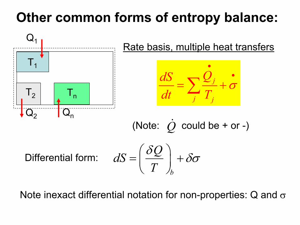
Other common forms of entropy balance:
T1
T2 Tn
Q1
QnQ2
j
j j
QdSdt T
σ
••
= +∑
Rate basis, multiple heat transfers
(Note: could be + or -)
b
QdSTδ δσ = +
Q
Differential form:
Note inexact differential notation for non-properties: Q and σ

Evaluating Entropy Production and Transfer
Absolute value of entropy production not as usefulas relative values: Can use this information to focusattention on components where most irreversibiltiesare produced
Example 6.2: Irreversible process of water
Example 6.3: Eval Min theoretical compression work
Example 6.4: Pinpointing Irrevs

Increase in Entropy Principle:Closed Systems
Show that the summation of the entropy changes of surroundings AND system must always increase or remain the same
] 0isol
E∆ =
System
Surroundings
Energy Transfer is Zero
Mass Transfer is Zero
The larger system is an ISOLATED SYSTEM
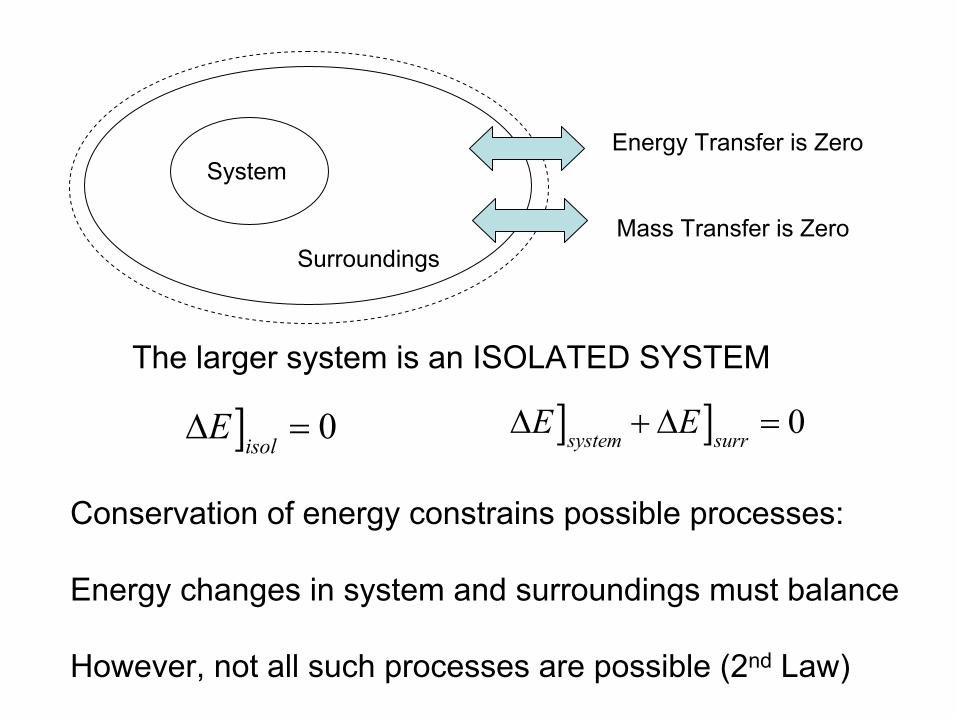
] 0isol
E∆ = ] ] 0system surr
E E∆ + ∆ =
System
Surroundings
Energy Transfer is Zero
Mass Transfer is Zero
The larger system is an ISOLATED SYSTEM
Conservation of energy constrains possible processes:
Energy changes in system and surroundings must balance
However, not all such processes are possible (2nd Law)

System
Surroundings
Energy Transfer is Zero
Mass Transfer is Zero
] 0isolisolS σ∆ = >
] ] 0isolsystem surrS S σ∆ + ∆ = >
]2
1isolisol
b
QSTδ σ ∆ = + ∫
0Adiabatic

System
Surroundings
Energy Transfer is Zero
Mass Transfer is Zero
] ] 0isolsystem surrS S σ∆ + ∆ = >
Only processes that can occur are when entropy of Isolated System INCREASES.
Entropy is Extensive: Entropy need NOT increase for BOTH System AND Surroundings, but SUM must increase.
Direction of process and feasibility constrained
Spontaneous processes tend to reach equilibrium- increasing S

Increase in Entropy Principle:Closed Systems
The summation of the entropy changes of surroundings AND system must always increase (or remain the same for ideal)
] ]totalsystem surrS S σ∆ + ∆ =
0 ideal0 actual0 impossible
total
total
total
σσσ
=><

Examples in Text
Example 6.5: Quenching metal bar
Statistical Interpretation of Entropy
Statistical Interpretation of Entropy

Entropy Rate Balance:Control Volumes
jcvi i e e CV
j i ej
QdS m s m sdt T
σ
•• • •
= + − +∑ ∑ ∑Rate of entropy change
Rates of entropy transferRate of entropy
production
Inlets, iExits, e
jTjQ
cvσ
In + Gen = Stored + Out
Entropy Rate Balance:Control Volumes
( )cv VS t sdVρ= ∫ j
Aj bj
Q q dAT T
=
∑ ∫
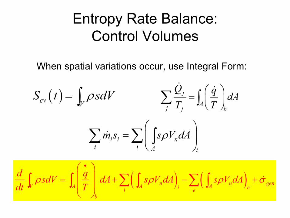
When spatial variations occur, use Integral Form:
( ) ( )n n genV A A Ai ei eb
d qsdV dA s V dA s V dAdt T
ρ ρ ρ σ•
= + − +
∑ ∑∫ ∫ ∫ ∫
i i ni i A i
m s s V dAρ
=
∑ ∑ ∫

Entropy Rate Balance:Control Volumes
At Steady-State
0 CVj
i i e ej i ej
Qm s m s
Tσ
•• • •
= + − +∑ ∑ ∑
Mass:
Energy:
Entropy:
i ei e
m m• •
=∑ ∑
2 2
02 2i e
cv cv i i i e e ei e
V VQ W m h gz m h gz• • • •
= − + + + − + +
∑ ∑
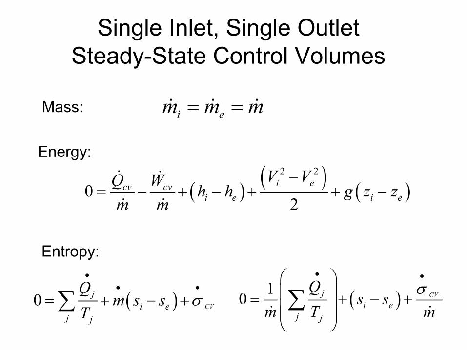
Single Inlet, Single OutletSteady-State Control Volumes
i em m m= =
( ) ( ) ( )2 2
02
i ecv cvi e i e
V VQ W h h g z zm m
−= − + − + + −
( )0 CV
ji e
j j
Qm s s
Tσ
•• •
= + − +∑
Mass:
Energy:
Entropy:
( )10 CVji e
j j
Qs s
m T mσ
• • = + − + ∑

Single Inlet, Single OutletSteady-State Control Volumes
Entropy: ( ) 1 CVje i
j j
Qs s
m T mσ
• • − = + ∑
( ) CVe is s
mσ•
− =
Entropy passing from inlet to exit can: increase, decreaseor remain constant. Second term RHS is positive or zero.
Entropy/mass can only decrease if NET entropy flow OUT with heat transfer exceeds entropy Generation IN control volume
When NO heat transfer (adiabatic):

Single Inlet, Single OutletSteady-State Control Volumes
( ) CVe is s
mσ•
− =When NO heat transfer (Adiabatic):
Entropy increases when IRREVERSIBILTY present
Entropy constant when REVERSIBLE: ISENTROPIC
e is s=
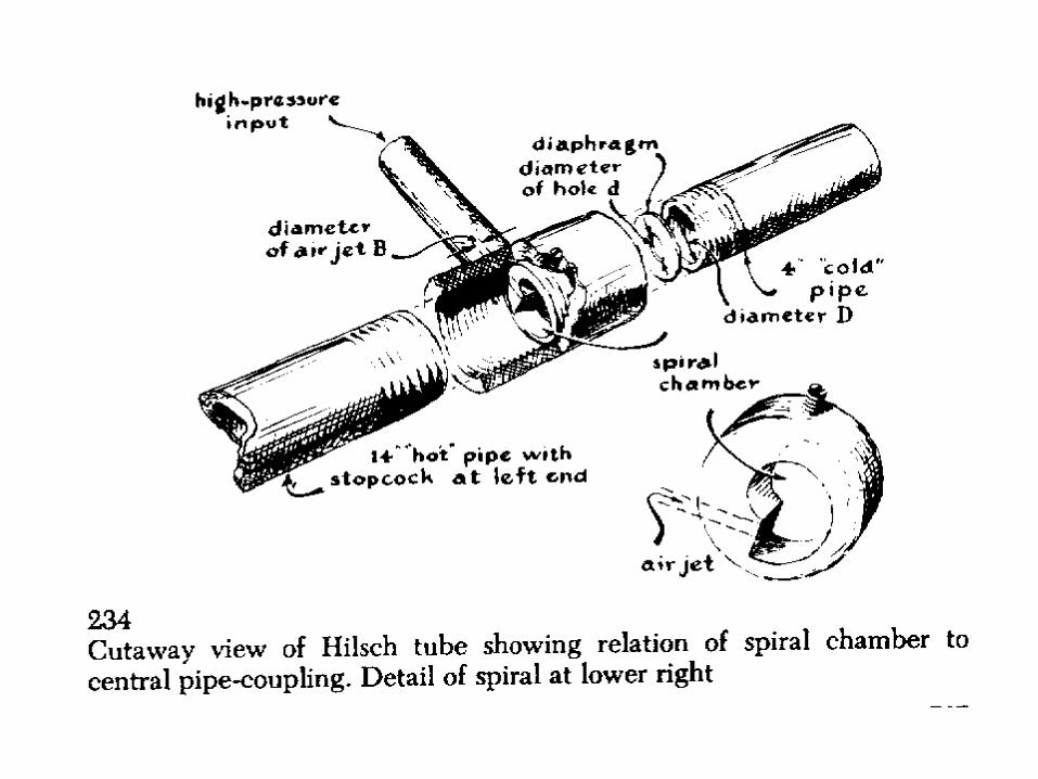


http://www.visi.com/~darus/hilsch/
Examples
6.6 Entropy production in a steam turbine
6.7 Evaluating a performance claim
6.8 Entropy production in heat pump components

Isentropic ProcessesShowing isentropic processes is rapid/easy
on T-s or h-s diagrams. Vertical lines:
However, tabular data may still be used as well.

Isentropic Processes
State 1 is in superheated region
P1 and T1 used to get s1
State 2 is in superheated region
Where s2 = s1. Use P2, T2, other
Isentropic process: s3 = s2 = s1 Use P3 or T3 to get ssat.
IF s3 < ssat, then state 3 is in saturated region.
Get quality, x3, then can get other properties.
Saturated Water
Table A-2, A3, A2E, A3E
T
v
f g
Superheated Vapor
Table A-4, A-4E
T
v
f g293 F
500 F
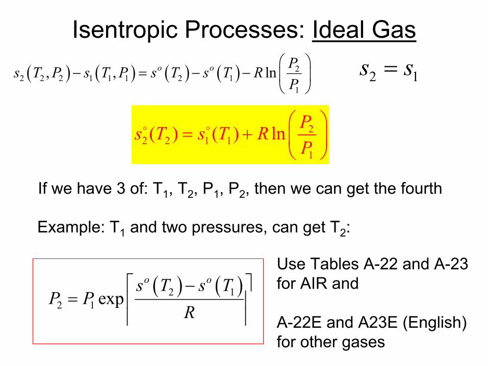
Isentropic Processes: Ideal Gas
( ) ( ) ( ) ( ) 22 2 2 1 1 1 2 1
1
, , lno o Ps T P s T P s T s T RP
− = − −
2 1s s=
22 2 1 1
1
( ) ( ) ln Ps T s T RP
= +
If we have 3 of: T1, T2, P1, P2, then we can get the fourth
Example: T1 and two pressures, can get T2:
Use Tables A-22 and A-23for AIR and
A-22E and A23E (English)for other gases
( ) ( )2 12 1 exp
o os T s TP P
R −
=
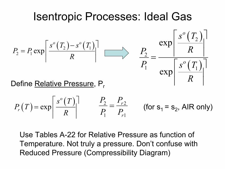
Isentropic Processes: Ideal Gas
( ) ( )2 12 1 exp
o os T s TP P
R −
=
( )
( )
2
2
1 1
exp
exp
o
o
s TRP
P s TR
=
( ) ( )expo
r
s TP T
R
=
Use Tables A-22 for Relative Pressure as function of Temperature. Not truly a pressure. Don’t confuse with Reduced Pressure (Compressibility Diagram)
2 2
1 1
r
r
P PP P
=
Define Relative Pressure, Pr
(for s1 = s2, AIR only)
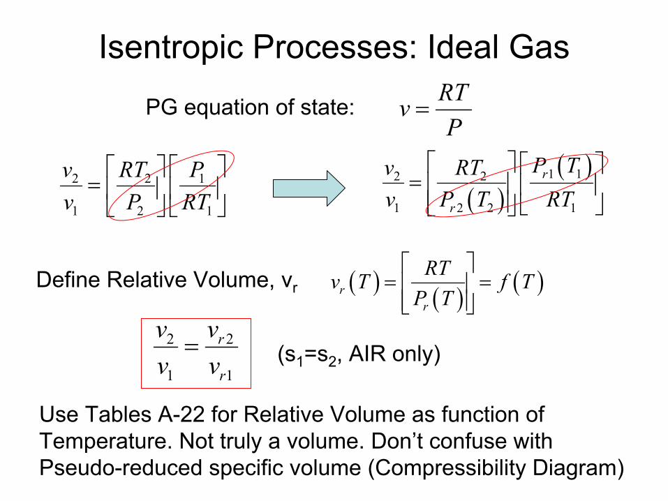
Isentropic Processes: Ideal GasRTvP
=PG equation of state:
2 2 1
1 2 1
v RT Pv P RT
= ( )
( )1 12 2
1 2 2 1
r
r
P Tv RTv P T RT
=
( ) ( ) ( )rr
RTv T f TP T
= =
Define Relative Volume, vr
Use Tables A-22 for Relative Volume as function of Temperature. Not truly a volume. Don’t confuse with Pseudo-reduced specific volume (Compressibility Diagram)
2 2
1 1
r
r
v vv v= (s1=s2, AIR only)
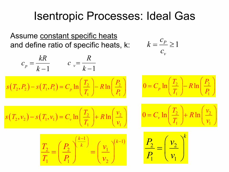
Isentropic Processes: Ideal Gas
( )1 1
2 2 1
1 1 2
k kkT P v
T P v
− −
= =
Assume constant specific heatsand define ratio of specific heats, k:
( ) ( ) 2 22 2 1 1
1 1
, , ln lnpT Ps T P s T P C RT P
− = −
( ) ( ) 2 22 2 1 1
1 1
, , ln lnvT vs T v s T v C RT v
− = +
2 2
1 1
0 ln lnvT vC RT v
= +
2 2
1 1
0 ln lnpT PC RT P
= −
1P
v
ckc
= ≥
1vRck
=−1p
kRck
=−
2 2
1 1
kP vP v
=

Examples:
6.9 Isentropic process in Air
6.10 Air leaking from tank

Isentropic EfficienciesComparing actual (adiabatic) and isentropic devices with
- same inlet states- same exit pressure
Turbines, compressors, nozzles and pumps
Isentropic turbine efficiency:
This helicopter gas turbine engine photo is courtesy of the U.S.Military Academy.
WTurbine
2
Turbine
1
WWTurbine
2
Turbine
1
Actual versusIsentropic

Isentropic Efficiencies(Adiabatic, Reversible)
Turbines
This helicopter gas turbine engine photo is courtesy of the U.S. Military Academy.
1st Law:
2nd Law:
1 2cvW h hm
•
• = −
WTurbine
2
Turbine
1
WWTurbine
2
Turbine
1
2 1 0cv s sm
σ•
• = − ≥
0.7 0.9Tη≤ ≤Typical:
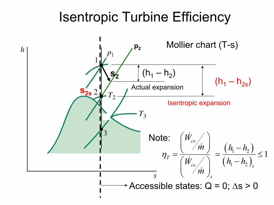
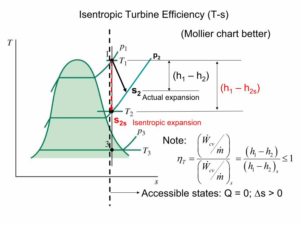
Isentropic Turbine Efficiency
( )( )
1 2
1 2
1cv
Tcv s
s
Wm h h
h hWm
η
− = = ≤
−
p2
s2
s2s
(h1 – h2)(h1 – h2s)
Accessible states: Q = 0; ∆s > 0
Isentropic expansion
Note:
Mollier chart (T-s)
Actual expansion
( )( )
1 2
1 2
1cv
Tcv s
s
Wm h h
h hWm
η
− = = ≤
−
p2
s2
s2s
(h1 – h2)(h1 – h2s)
Accessible states: Q = 0; ∆s > 0
Actual expansion
Isentropic expansion
Note:
Isentropic Turbine Efficiency (T-s)
(Mollier chart better)

Compressors and Pumps
Rotating compressors
Reciprocating compressor
Common Form of 1st Law:
( ) ( )2 2
1 21 2 1 22
W V Vh h g z zm
•
•
−= − + + −
[ W < 0 ]

s2
( )( )
2 1
2 1
1
cv
ssc
cv
Wm h h
h hWm
η
− − = = ≤
− −
p1s2s
(h2s – h1)
(h2 – h1)
Accessible states: Q = 0; ∆s > 0
Actual compression
Isentropic compression
Note:
p2
T2
T1s1
Isentropic Compressor Efficiency (Gases)
h
Liquid

Isentropic Efficiencies: Compressors (Gases) and Pumps (Liquids)
Typical Isentropic Efficiencies of Compressors and Pumps:
Pumps, assuming incompressible model:(will consider more detail later)
( )2 1
2 1
sP
v P Ph h
η−
=−
0.75 0.85cη≤ ≤
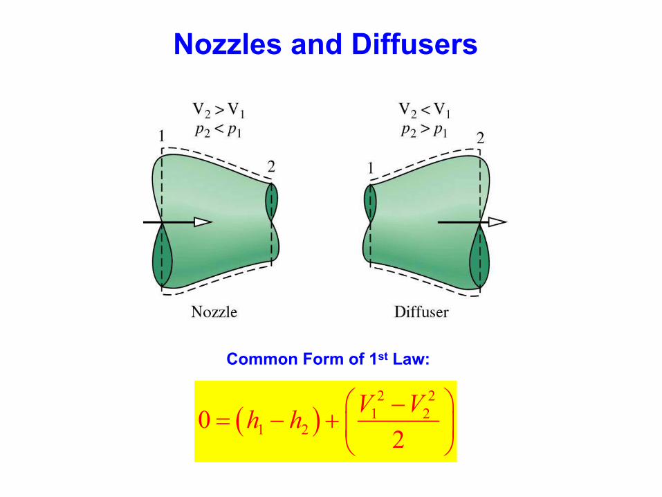
Nozzles and Diffusers
( )2 2
1 21 20
2V Vh h −
= − +
Common Form of 1st Law:
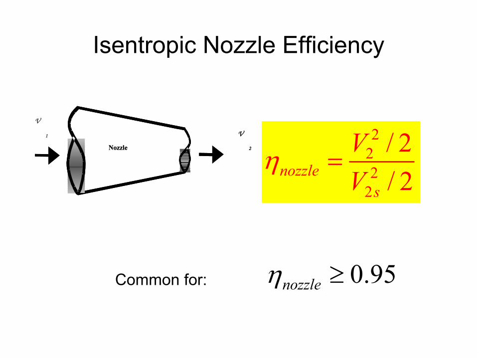
Isentropic Nozzle Efficiency
V
1
Nozzle
V
2Nozzle
V
2
222
2
/ 2/ 2nozzle
s
VV
η =
0.95nozzleη ≥Common for:

Examples:
6.11 Eval turbine work using Isentropic efficiency
6.12 Eval Isentropic turbine efficiency
6.13 Eval Isentropic nozzle efficiency
6.14 Eval Isentropic compressor efficiency
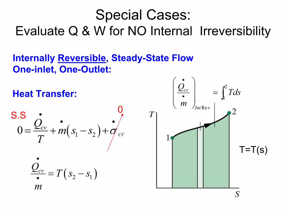
Special Cases: Evaluate Q & W for NO Internal Irreversibility
Internally Reversible, Steady-State FlowOne-inlet, One-Outlet:
( )2 1cvQ T s sm
•
• = −
Heat Transfer:
( )1 20 CVcvQ m s sT
σ•
• •
= + − +
0
2
1
Re
cv
Int v
Q Tdsm
•
•
=
∫
T=T(s)
S.S
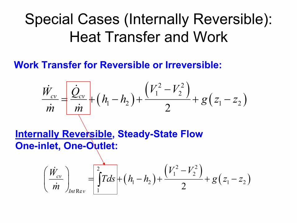
Special Cases (Internally Reversible): Heat Transfer and Work
( ) ( ) ( )2 22
1 21 2 1 2
1Re 2cv
Int v
V VW Tds h h g z zm
− = + − + + −
∫
Internally Reversible, Steady-State FlowOne-inlet, One-Outlet:
Work Transfer for Reversible or Irreversible:
( ) ( ) ( )2 2
1 21 2 1 22
cv cvV VW Q h h g z z
m m
−= + − + + −
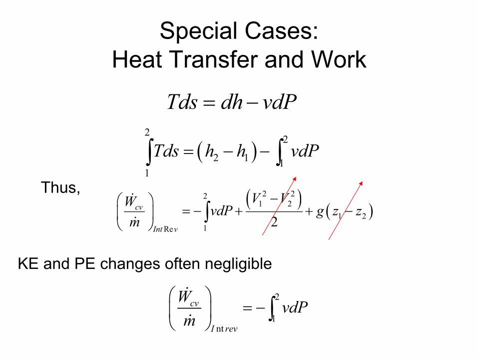
Special Cases: Heat Transfer and Work
Tds dh vdP= −
( )2
2
2 1 11
Tds h h vdP= − −∫ ∫( ) ( )
2 221 2
1 21Re 2
cv
Int v
V VW vdP g z zm
− = − + + −
∫
Thus,
2
1nt
cv
I rev
W vdPm
= −
∫
KE and PE changes often negligible
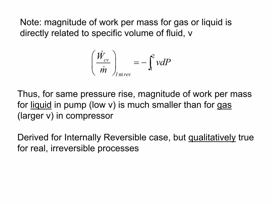
2
1nt
cv
I rev
W vdPm
= −
∫
Note: magnitude of work per mass for gas or liquid isdirectly related to specific volume of fluid, v
Thus, for same pressure rise, magnitude of work per mass for liquid in pump (low v) is much smaller than for gas(larger v) in compressor
Derived for Internally Reversible case, but qualitatively truefor real, irreversible processes
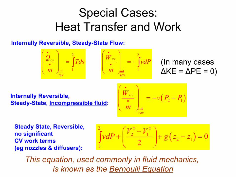
Special Cases: Heat Transfer and Work
Internally Reversible, Steady-State Flow:
2
1intrev
cvQ Tdsm
•
•
=
∫2
1intrev
cvW vdPm
•
•
= −
∫ (In many cases∆KE = ∆PE = 0)
Internally Reversible, Steady-State, Incompressible fluid:
( )2 1
intrev
cvW v P Pm
•
•
= − −
Steady State, Reversible,no significant CV work terms(eg nozzles & diffusers):
( )2 2 2
2 12 1
1
02
V VvdP g z z −+ + − =
∫
This equation, used commonly in fluid mechanics, is known as the Bernoulli Equation
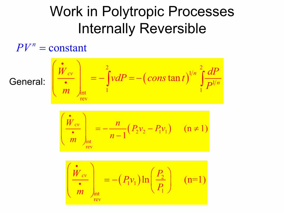
Work in Polytropic ProcessesInternally Reversible
( )2 2 1 1
intrev
(n 1)1
cvW n P v Pvnm
•
•
= − − ≠
−
constantnPV =
( ) 21 1
1intrev
ln (n=1)cvW PPvPm
•
•
= −
( )2 2
11
1 1intrev
tan ncvn
W dPvdP cons tPm
•
•
= − = −
∫ ∫General:

Work in Polytropic Processes: Ideal Gas
( )2 2 1 1
intrev
(n 1)1
cvW n P v Pvnm
•
•
= − − ≠
−
1
2 2
1 1
kkT P
T P
−
=
constantnPV =
For Ideal Gases:
( )2 1
intrev
(ideal gas, 1)1
cvW nR T T nnm
•
•
= − − ≠
−
( )1
1 2
1intrev
1 (ideal gas, n 1)1
n ncvW nRT P
n Pm
• −
•
= − − ≠ −
Equivalent to:
2
1intrev
ln (ideal gas, n=1)cvW PRTPm
•
•
= −
Where:

Examples:
6.15 Polytropic compression of air

END


![The steam-turbine expansion line on the Mollier diagram ... · Buckingham] TheReheatFactor 581 LetTobethekineticenergyperunitmassatAo,oftheaxial component ^ofthevelocity,andTthecorrespondingquantityat](https://img.pdfslide.us/doc/110x75/5c8b2a5809d3f2fa728bdd21/the-steam-turbine-expansion-line-on-the-mollier-diagram-buckingham-thereheatfactor.jpg)