Embed Size (px)
Citation preview
Chapter 6: The Role of Transportation in Economic Geography
• Transport Eras
• Transport Rates
• World Transportation Patterns
• Summary

Transport Eras - Taaffe’s Schema
• Local era: pre-railroad and prior to opening of the Erie Canal in 1825
• Trans-Appalachian era: canals and railroads up to ca. 1860 (Figure 6.1)
• Era of railroad dominance (ca. 1860 to World War II) Rise of gateway cities
• Competitive era: multi-modal
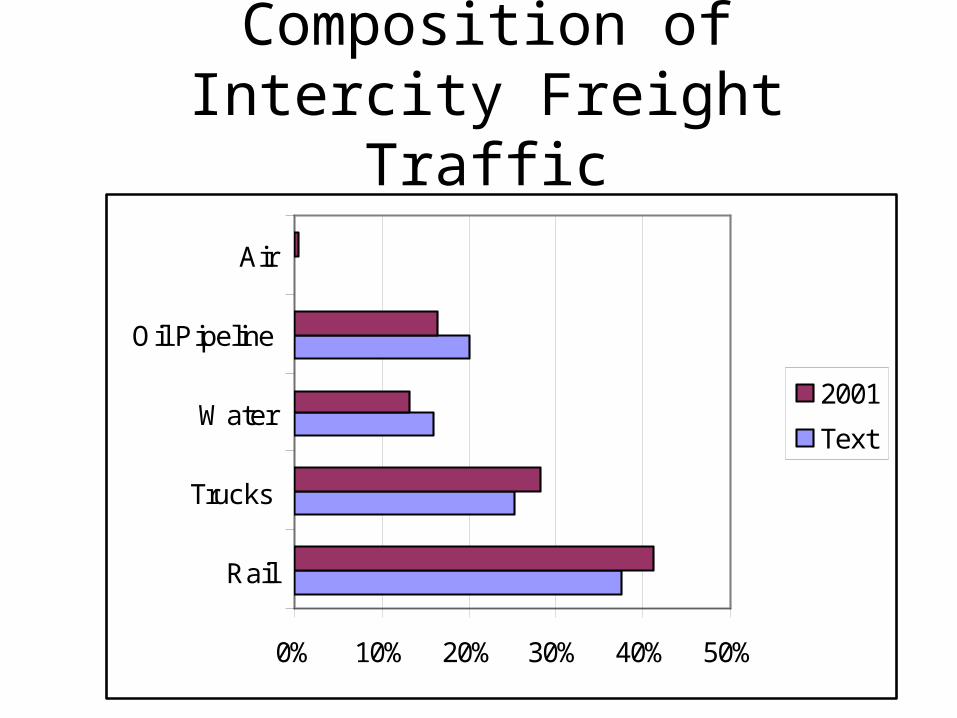
Composition of Intercity Freight Traffic
0% 10% 20% 30% 40% 50%
Rail
Trucks
Water
Oil Pipeline
Air
2001
Text

Freight Outlays (Shares of total)
0 0.2 0.4 0.6 0.8 1
Rail
Motor Truck
Oil Pipeline
Water
Air
2001
Text

Revenue Per Ton-Mile
0 10 20 30 40 50
Air
Rail
Motor Truck
Oil Pipeline
Water
1997
Text

Fixed & Variable (Operating) Costs
Mode Fixed/Capital Costs Operating CostsRail or Highway Land, Construction,
Rolling StockMaintenance, Labor, Fuel
Pipeline Land, Construction Maintenance, EnergyAir Land, Field & Terminal
Construction, AircraftMaintenance, Fuel, Labor
Sea Land for Port Terminals,Cargo HandlingEquipment, Ships
Maintenance, Labor, Fuel
Pedestrian/Bikeway Land, Construction Maintenance

The Structure of Transport Costs
Terminal Costs versus Line Haul Costs
- buildings, docks, handling
Distance
Tra
nsp
ort
Cos
t / M
ile
Terminal Cost $5Line Haul Cost $.25/ton-mile
$5.25
1 100
$.30
Tot
al T
ran
spor
t C
ost/
Uni
t W
eigh
t
Distance
Linear
O
T
Tapering

Variations in Transport Costs Among Modes
Distance
Tra
nsp
ort
Cos
t/U
nit
Wei
ght
Truck
Rail
ShipPipeline
Air
T R S

Factors Influencing Transport Rates1. Grouping freight rates into zones (fig 3.14)
2. Variations due to commodity characteristics
(a) Differences in cost of service related to:
(1) Loading characteristics
(2) Size of shipment
(3) Perishability and risk of damage
(b) Elasticity of Demand for Transportation (Box3-1)
3. Variations due to traffic characteristics
(a) intermodal competition
(b) traffic density
(c) direction of haul

Freight Rate Zones

Demand Elasticity$
Q
Elastic
$
Q
PerfectlyInelastic
Q
$ PerfectlyElastic

General Relationship Between Distance and Unit Cost
Distance
Quantity
$

Tapered Freight Rates Can Alter Market Areas
A BM M* M**

Freight Rates Can Create Overlapping Market Boundaries:
Demand Cones from Places A & B
Place A Place BS T
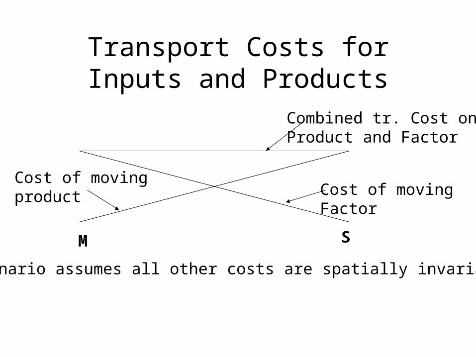
Transport Costs for Inputs and Products
M S
Combined tr. Cost onProduct and Factor
Cost of movingFactor
Cost of movingproduct
Scenario assumes all other costs are spatially invariant
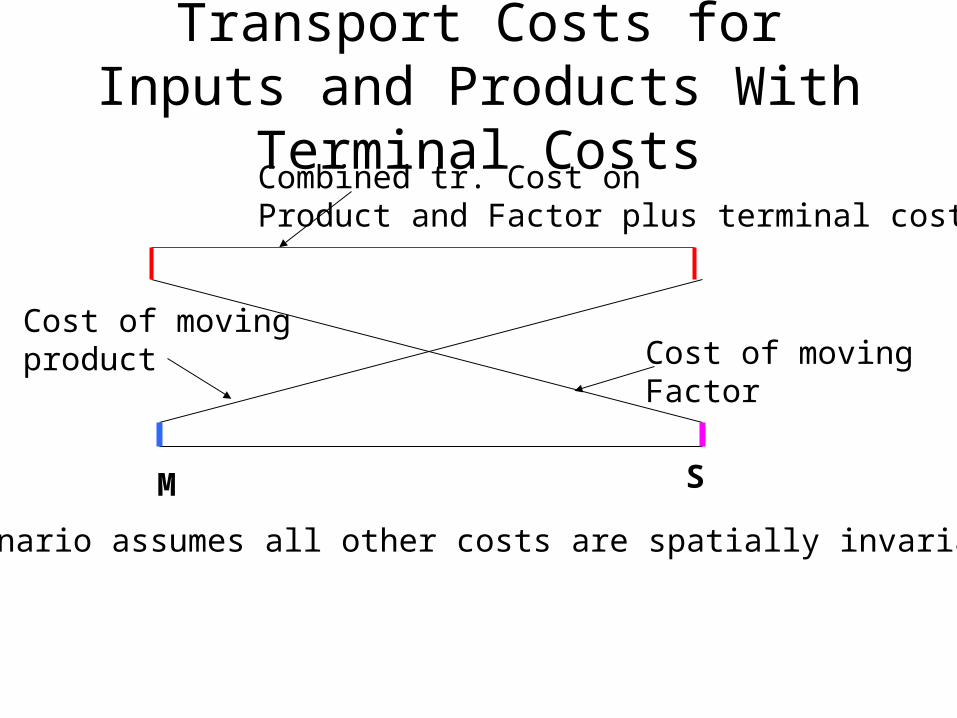
Transport Costs for Inputs and Products With Terminal Costs
M S
Combined tr. Cost onProduct and Factor plus terminal costs
Cost of movingFactor
Cost of movingproduct
Scenario assumes all other costs are spatially invariant

Effects on the Location of Production
General Tendency to Pull Away from Intermediate Locations
Market Material
S
TX
Y
GH
Impact on spacing of isotims – concept coming

Tapered Transport Costs Pull Mfg. towards markets or
materials--But:1. Intermodal “break of bulk” locations
2. In-transit privileges - lower rate for long haul granted to raw and processed materials
Material MarketTransshipmentLocation
MaterialTr. Cost
Product Tr. Cost

Isotims and Isodapanes

Smith’s Space-Cost Model

Spatial Pricing Policies
A. FOB - Free On Board - Consumer pays full cost of transport
B. Discriminatory
(1) Uniform delivered pricing (CIF)
(2) Basing point
(3) Spatially discriminatory pricing
(market segmentation)
(4) dumping

Typical F.O.B. Market
X YB B*
T
A R
S

Basing Point Pricing
PBasing Point
R
S
T
X
A
BC
Phantom Freight
M
Distance
O

General Pricing Principle
• Producers choose location to maximize
profit
• Profit = Total Revenue – Total Costs
• Total Revenue = sum of revenues from various geographic markets
• Total Costs = sum of costs for all input factors and transportation costs

Hypothetical Example Total, Average & Marginal Cost Relations
Production/ Sales
QuantityCOST
MarginalCOST Total
COST Average
REVENUE Marginal
REVENUE Total
REVENUE Average Profit
1 10 10 10 12 12 12 22 8 18 9 11 23 11.5 53 6 24 8 10 33 11 94 5 29 7.25 9 42 10.5 135 4 33 6.6 8 50 10 176 5 38 6.33 7 57 9.5 197 6 44 6.29 6 63 9 198 7 51 6.38 5 68 8.5 179 8 59 6.56 4 72 8 13
10 9 68 6.8 3 75 7.5 7

Graph of Hypothetical Example
0
2
4
6
8
10
12
14
1 2 3 4 5 6 7 8 9 10
Quantity
$
COST Marginal
COST Average
REVENUEMarginal
REVENUEAverage
Po
Qo

Market Segmentation & Dumping
$
Q
ACMC
ARMR
ARA
P
Q*
MRA
QA
PA
ARBMRB
QB
PB