Chapter 6

The production process

Choice of technology

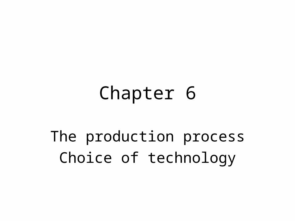
The Production Process

• Production technology relates inputs to outputs. – Labor-intensive technology: Technology that

relies heavily on human labor rather than capital.– Capital-intensive technology: Technology that

relies heavily on capital rather than human labor

• The optimal method of production, for a profit-maximizing firm, is the one that minimizes costs.

There are three important ways to measure the productivity of inputs:

• Total product (TP)

• Average product (AP)

• Marginal product (MP)

Total Product (TP) Function

• Production function or total product function: – A mathematical or numerical expression of a

relationship between inputs and outputs– Shows units of total product as a function of

units of inputs.

Average Product (AP)

• The average amount of output produced by each unit of a variable factor of production

• Output per unit of an input.

laborofunitstotal

producttotallaborofproductAverage

Marginal Product (MP)

• The additional output that can be produced by adding one more unit of a specific input, ceteris paribus.

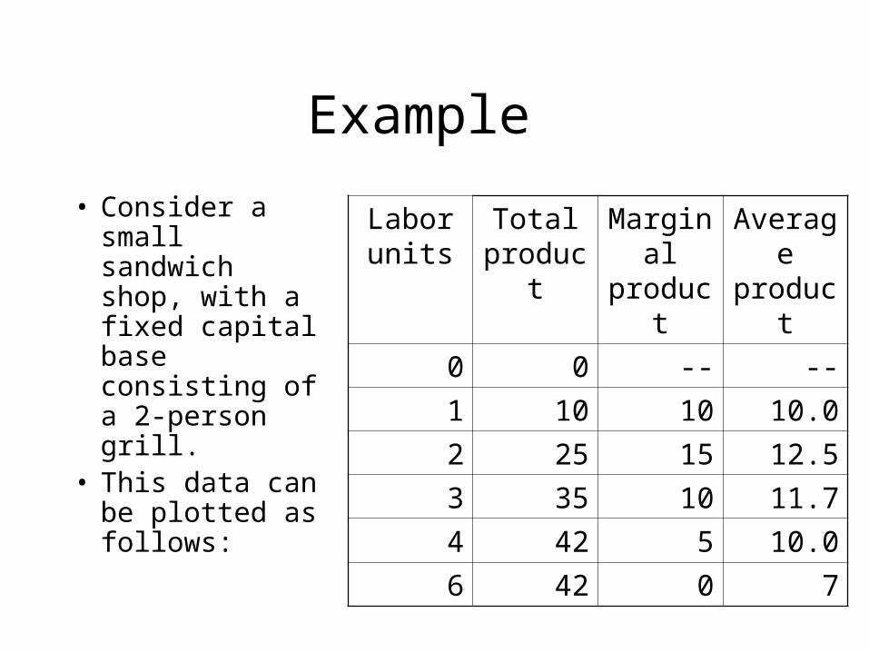
Example

• Consider a small sandwich shop, with a fixed capital base consisting of a 2-person grill.

• This data can be plotted as follows:

Labor units

Total product

Marginal product

Average product

0 0 -- --

1 10 10 10.0

2 25 15 12.5

3 35 10 11.7

4 42 5 10.0

6 42 0 7

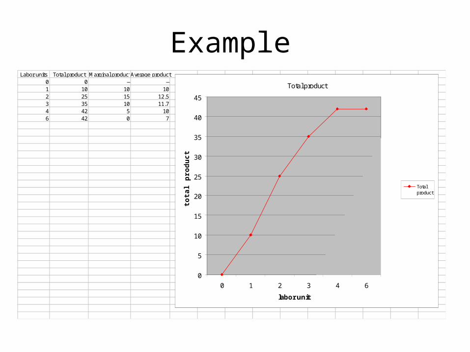
Example Labor units Total product Marginal productAverage product

0 0 -- --1 10 10 102 25 15 12.53 35 10 11.74 42 5 106 42 0 7

Total product

0

5

10

15

20

25

30

35

40

45

0 1 2 3 4 6

labor unit

tota

l pro

du

ct

Totalproduct

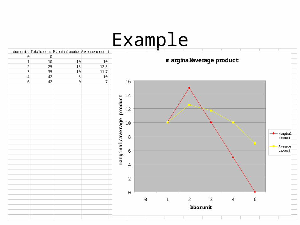
ExampleLabor units Total productMarginal productAverage product

0 01 10 10 102 25 15 12.53 35 10 11.74 42 5 106 42 0 7

marginal/average product

0

2

4

6

8

10

12

14

16

0 1 2 3 4 6

labor unit

ma

rgin

al/a

ve

rag

e p

rod

uc

t

Marginalproduct

Averageproduct

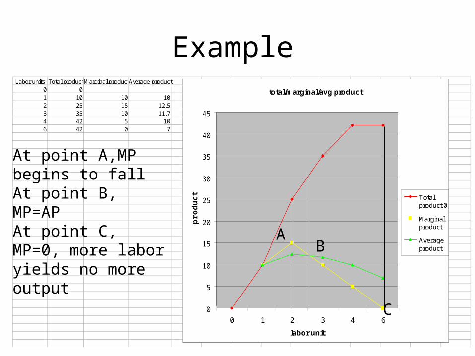
Example Labor units Total productMarginal productAverage product

0 01 10 10 102 25 15 12.53 35 10 11.74 42 5 106 42 0 7

total/marginal/avg product

0

5

10

15

20

25

30

35

40

45

0 1 2 3 4 6

labor unit

pro

du

ct Total

product 0

Marginalproduct

Averageproduct

A B

C

At point A,MP begins to fallAt point B, MP=APAt point C, MP=0, more labor yields no more output

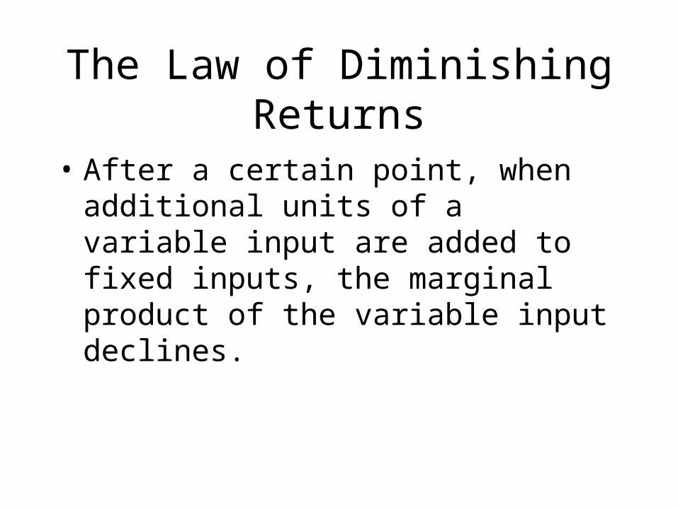
The Law of Diminishing Returns

• After a certain point, when additional units of a variable input are added to fixed inputs, the marginal product of the variable input declines.

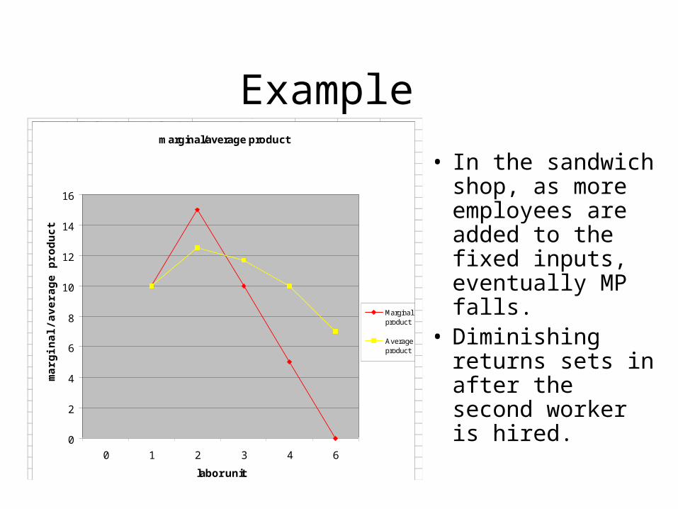
Example

• In the sandwich shop, as more employees are added to the fixed inputs, eventually MP falls.

• Diminishing returns sets in after the second worker is hired.

Labor units Total productMarginal productAverage product0 01 10 10 102 25 15 12.53 35 10 11.74 42 5 106 42 0 7

marginal/average product

0

2

4

6

8

10

12

14

16

0 1 2 3 4 6

labor unit

ma

rgin

al/a

ve

rag

e p

rod

uc

t

Marginalproduct

Averageproduct

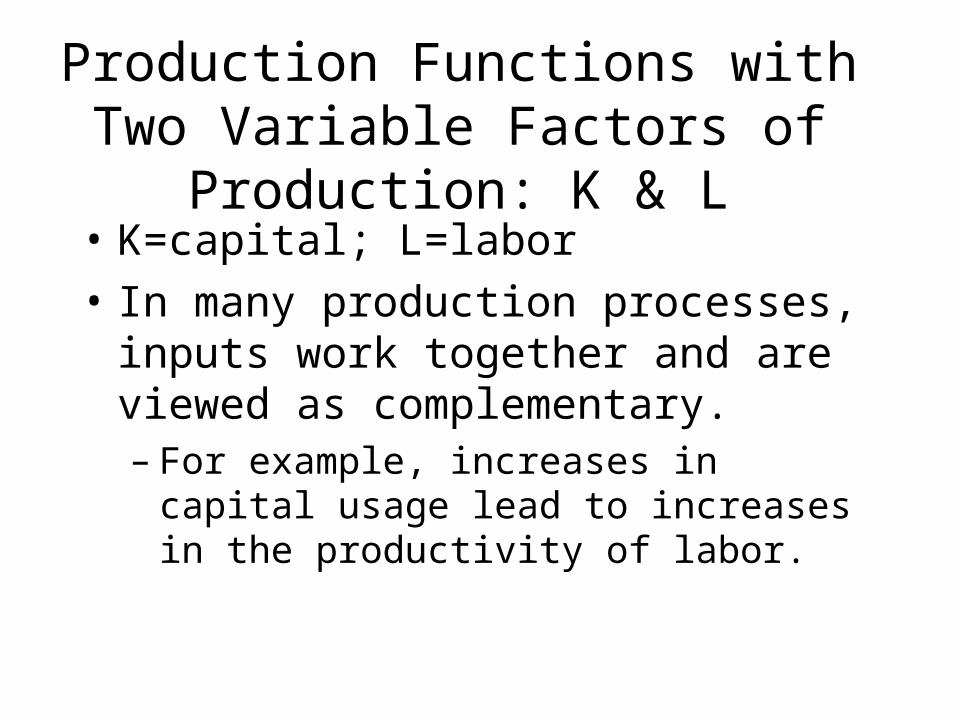
Production Functions with Two Variable Factors of Production: K & L

• K=capital; L=labor

• In many production processes, inputs work together and are viewed as complementary.– For example, increases in capital usage lead to

increases in the productivity of labor.

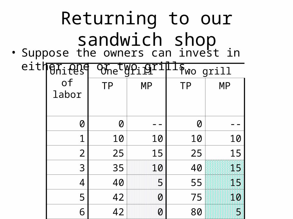
Returning to our sandwich shop• Suppose the owners can invest in either one or two grills.

Unites of labor

One grill Two grill

TP MP TP MP

0 0 -- 0 --

1 10 10 10 10

2 25 15 25 15

3 35 10 40 15

4 40 5 55 15

5 42 0 75 10

6 42 0 80 5

7 42 0 80 0

Returning to our sandwich shop

• Notice that the MP of labor is higher with two grills than it is with one grill.

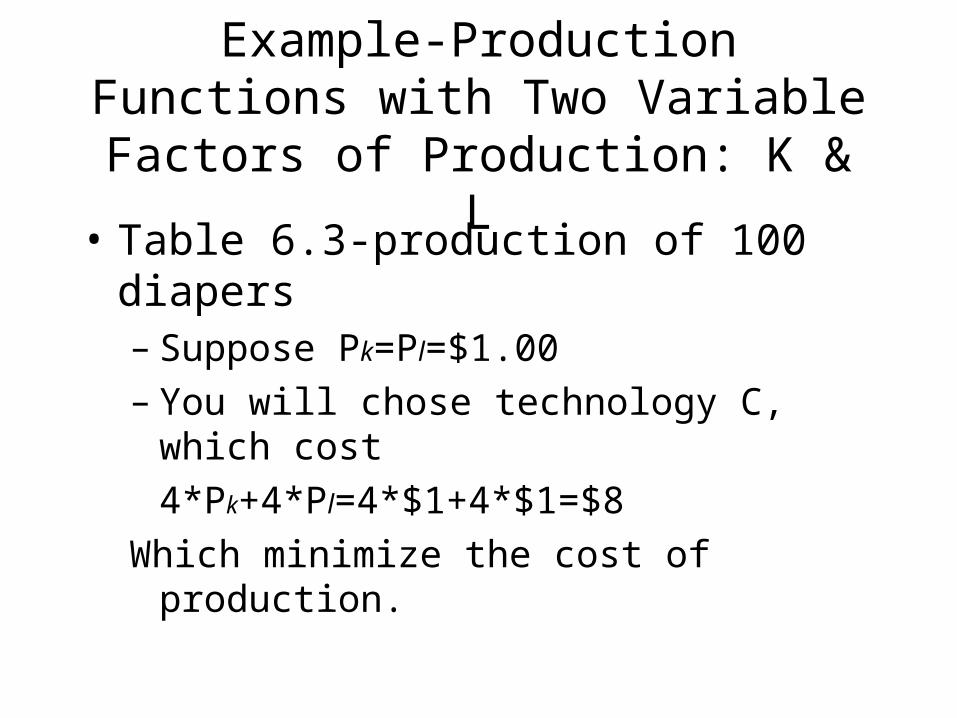
Example-Production Functions with Two Variable Factors of Production: K & L

• Table 6.3-production of 100 diapers– Suppose Pk=Pl=$1.00– You will chose technology C, which cost

4*Pk+4*Pl=4*$1+4*$1=$8

Which minimize the cost of production.

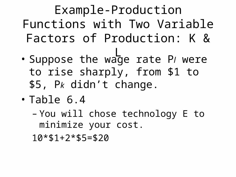
Example-Production Functions with Two Variable Factors of Production: K & L

• Suppose the wage rate Pl were to rise sharply, from $1 to $5, Pk didn’t change.

• Table 6.4– You will chose technology E to minimize your

cost.

10*$1+2*$5=$20

Chapter Summary

• Profit-maximizing, perfectly competitive firms face a perfectly elastic demand curve.

• A firm’s profits might be normal or economic, positive or negative.

• Total, average, and marginal product are three ways of measuring the productivity of an input.

• The law of diminishing returns states that in the short run, marginal product will eventually decline.

Chapter 7

Short-Run Costs and Output Decisions

Costs in the Short Run

• Short run: A period of time so short that some of the firm’s inputs are fixed in total supply.

• There are several ways to categorize short-run costs...

Fixed Costs (FC)

• Any cost that a firm bears in the short run that does not depend on its level of output. These costs are incurred even if the firm is producing nothing. There are no fixed cost in the long run.

• Sometimes called sunk costs because firms have no control over fixed costs in the short run.

Variable Costs (VC)

• Any cost that a firm bears that depends on the level of production chosen.

Total Costs (TC)

• Total Costs=Total Fixed Costs (TFC) +

Total Variable Costs (TVC)

• TC = TFC + TVC

FC-Total fixed cost (TFC)

• The total of all costs that do not change with output, even if output is zero.

FC-Average Fixed Costs (AFC)

• AFC = Total Fixed Costs

• q=quantity of output

q

TFCAFC

VC-total variable cost(TVC)

• Total variable cost: the total of all costs that vary with output in the short run

VC-Average Variable Costs (AVC)

• AVC = Total Variable Costs

• q=quantity of output

q

TVCAVC

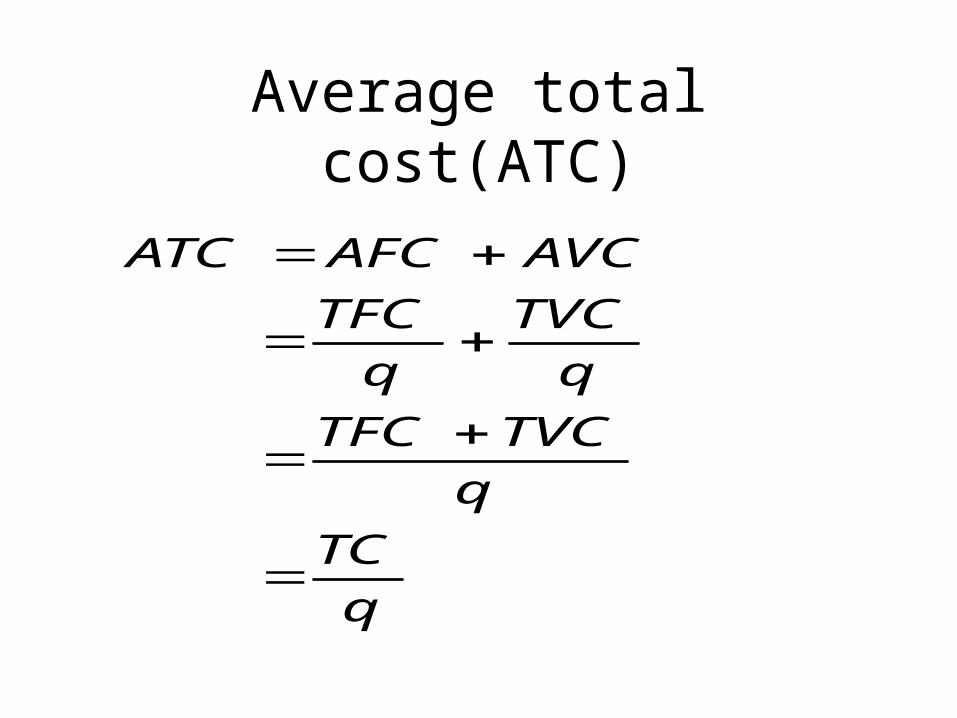
Average total cost(ATC)

q

TC

q

TVCTFC

q

TVC

q

TFC

AVCAFCATC

Marginal Costs (MC)

• The increase in total cost that results from producing one more unit of output

• Marginal costs reflect changes in variable costs.

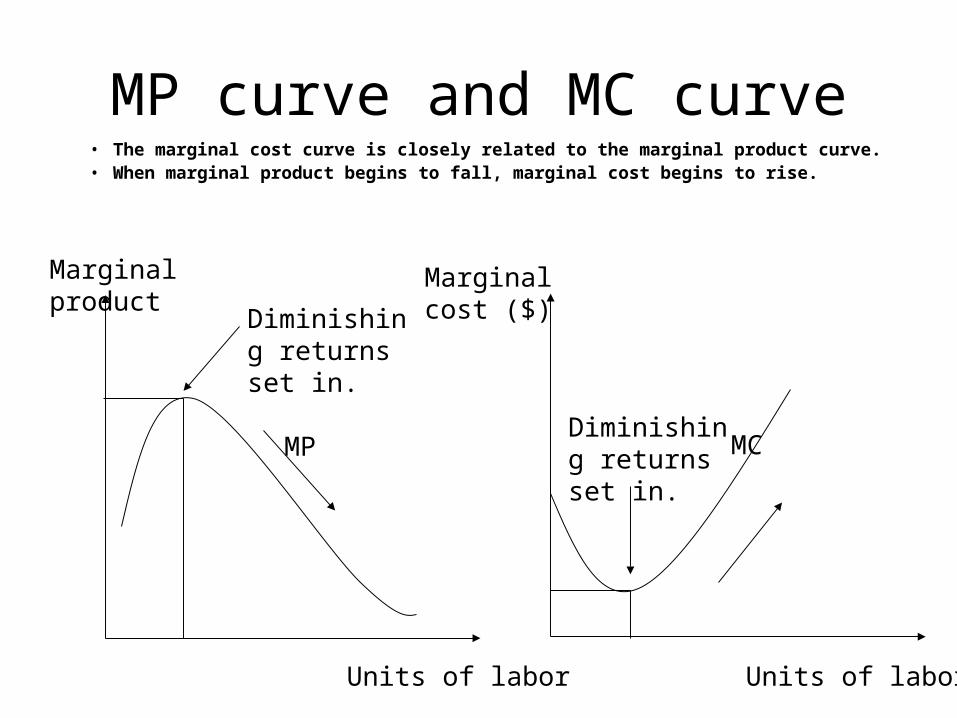
MP curve and MC curve• The marginal cost curve is closely related to the marginal product curve.• When marginal product begins to fall, marginal cost begins to rise.

Marginal product

Units of labor

MP

Units of labor

MC

Marginal cost ($)

Diminishing returns set in.

Diminishing returns set in.

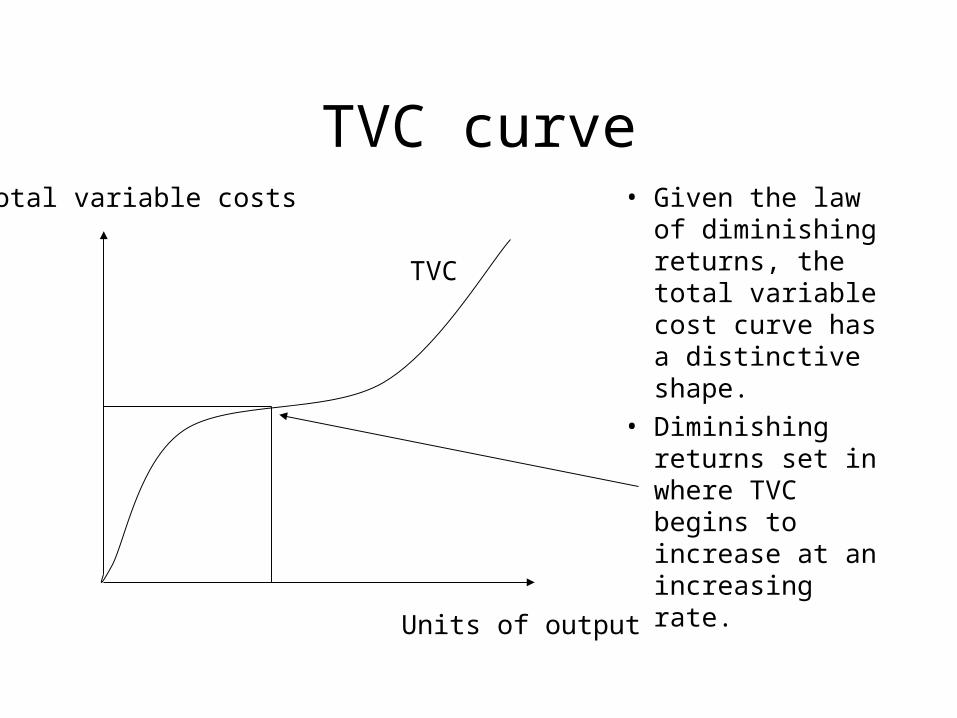
TVC curve• Given the law of

diminishing returns, the total variable cost curve has a distinctive shape.

• Diminishing returns set in where TVC begins to increase at an increasing rate.

Total variable costs

Units of output

TVC

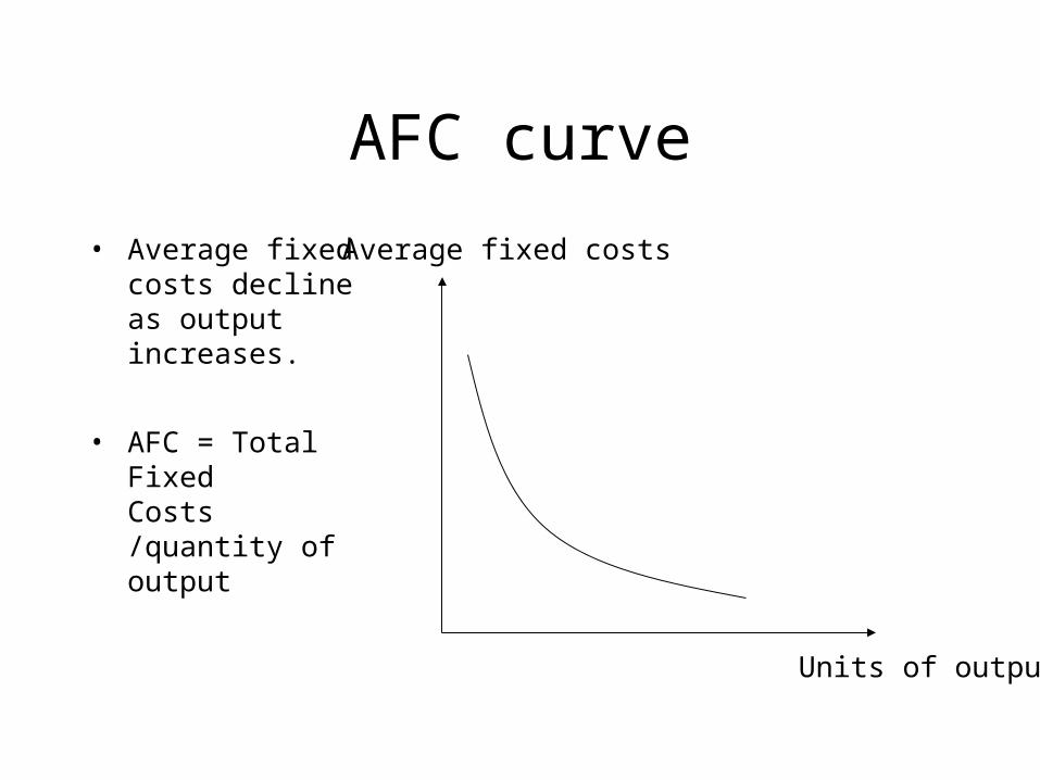
AFC curve

• Average fixed costs decline as output increases.

• AFC = Total Fixed Costs /quantity of output

Units of output

Average fixed costs

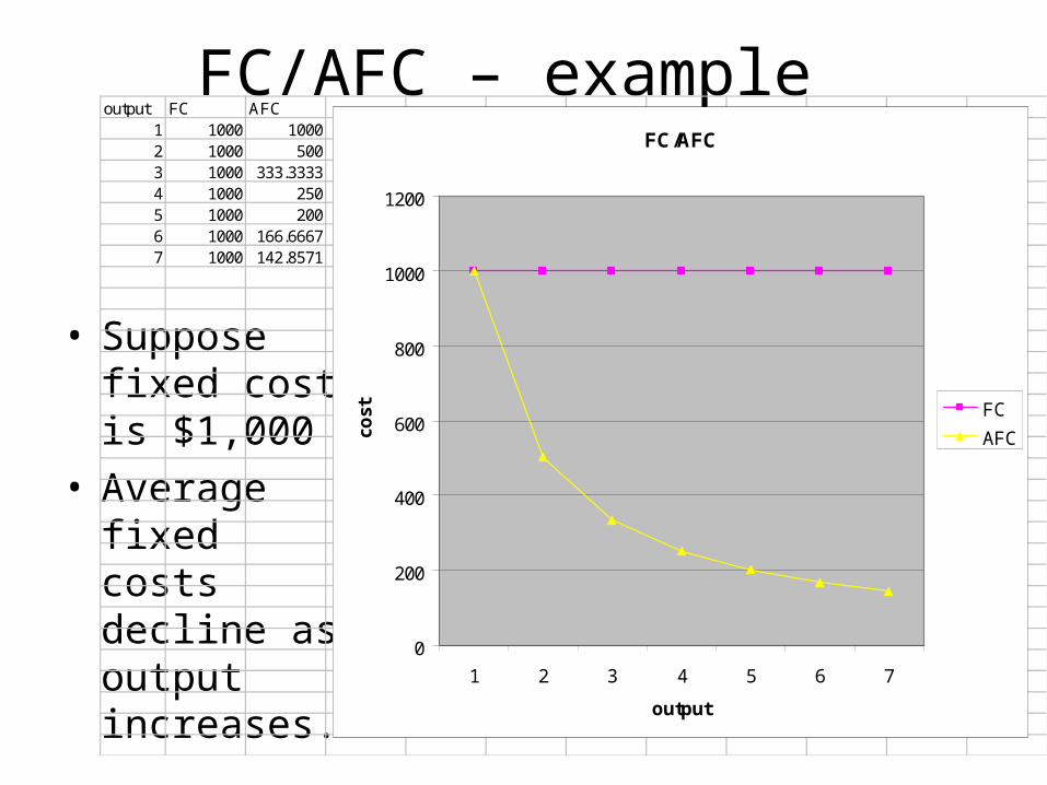
FC/AFC – example

• Suppose fixed cost is $1,000

• Average fixed costs decline as output increases.

output FC AFC1 1000 10002 1000 5003 1000 333.33334 1000 2505 1000 2006 1000 166.66677 1000 142.8571

FC/AFC

0

200

400

600

800

1000

1200

1 2 3 4 5 6 7

output

cost FC

AFC

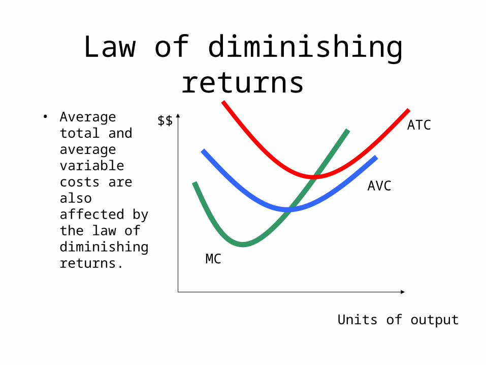
Law of diminishing returns

• Average total and average variable costs are also affected by the law of diminishing returns.

Units of output

$$

AVC

MC

ATC

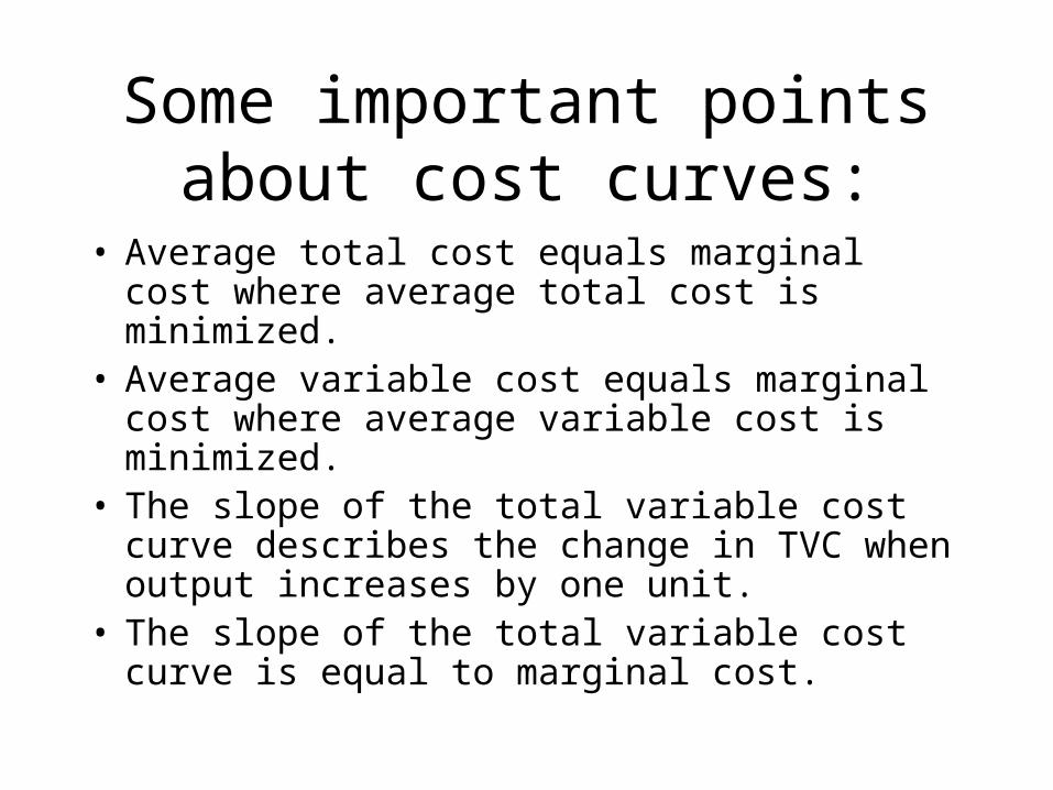
Some important points about cost curves:

• Average total cost equals marginal cost where average total cost is minimized.

• Average variable cost equals marginal cost where average variable cost is minimized.

• The slope of the total variable cost curve describes the change in TVC when output increases by one unit.

• The slope of the total variable cost curve is equal to marginal cost.

Review questions

• Know the shapes of TP, MP, AP curves• Choose the technology to minimize cost.• Know FC, TFC, AFC, VC, TVC, AVC, MC and

their curves.• The law of diminishing returns of both chapters.• Important points about cost curves.• In this quiz, you will be only tested on the

knowledge of chapter 7. Next quiz will be the test on chapter 8.