Chapter 6Simulation of Heat Transportin Low-Dimensional Oscillator Lattices

Lei Wang, Nianbei Li, and Peter Hänggi

Abstract The study of heat transport in low-dimensional oscillator lattices presentsa formidable challenge. Theoretical efforts have been made trying to reveal theunderlying mechanism of diversified heat transport behaviors. In lack of a unifiedrigorous treatment, approximate theories often may embody controversial pre-dictions. It is therefore of ultimate importance that one can rely on numericalsimulations in the investigation of heat transfer processes in low-dimensionallattices. The simulation of heat transport using the non-equilibrium heat bath methodand the Green-Kubo method will be introduced. It is found that one-dimensional(1D), two-dimensional (2D) and three-dimensional (3D) momentum-conservingnonlinear lattices display power-law divergent, logarithmic divergent and constantthermal conductivities, respectively. Next, a novel diffusion method is also intro-duced. The heat diffusion theory connects the energy diffusion and heat conductionin a straightforward manner. This enables one to use the diffusion method toinvestigate the objective of heat transport. In addition, it contains fundamentalinformation about the heat transport process which cannot readily be gatheredotherwise.

L. Wang (�)Department of Physics and Beijing Key Laboratory of Opto-electronic FunctionalMaterials and Micro-nano Devices, Renmin University of China, Beijing 100872,People’s Republic of Chinae-mail: phywanglei@ruc.edu.cn

N. LiCenter for Phononics and Thermal Energy Science, School of Physics Science and Engineering,Tongji University, Shanghai 200092, People’s Republic of Chinae-mail: nbli@tongji.edu.cn

P. HänggiInstitute of Physics, University of Augsburg, Augsburg 86135, Germanye-mail: Peter.Hanggi@physik.uni-augsburg.de

© Springer International Publishing Switzerland 2016S. Lepri (ed.), Thermal Transport in Low Dimensions, Lecture Notesin Physics 921, DOI 10.1007/978-3-319-29261-8_6

239

240 L. Wang et al.

6.1 Simulation of Heat Transport with Non-equilibrium HeatBath Method and Equilibrium Green-Kubo Method

We start out by considering numerically heat transport in typical momentum-conserving nonlinear lattices, from 1D to 3D. The numerical simulations areperformed with two different methods: the non-equilibrium heat bath method andthe celebrated equilibrium Green-Kubo method. Our major focus will be on thelength dependence of thermal conductivities where the asymptotic behavior towardsthe thermodynamic limit is of prime interest. As a result, numerical simulationsare usually taken on lattices employing very large up to even huge system sizes.Therefore, in order to get a compromise between better numerical accuracy andacceptable computational cost, a 5-th order Runge-Kutta algorithm [1] is appliedfor the simulations of the dissipative systems in the former case, while an embeddedRunge-Kutta-Nystrom algorithm of orders 8(6) [2, 3] is applied for the simulationsof the conservative Hamiltonian systems in the latter case.

6.1.1 Power-Law Divergent Thermal Conductivity in 1DMomentum-Conserving Nonlinear Lattices

Heat conduction induced by a small temperature gradient is expected to satisfy theFourier’s law in the stationary regime:

j D ��rT; (6.1)

where j denotes the steady state heat flux, rT denotes the small temperaturegradient, and � denotes the thermal conductivity. In practical numerical simulations,the temperature difference �T is usually fixed for convenience. In this setup, for asystem with length L, the steady state heat flux j should be inversely proportionalto L: j D ���T=L, if Fourier’s law is obeyed and � is a constant. However, formany 1D momentum-conserving lattices [4, 5], it is numerically found that j decaysas L�1C˛ with a positive ˛. This finding indicates that the thermal conductivity �is length dependent and diverges with L as � / L˛ in the thermodynamical limitL ! 1. The Fourier’s law is broken and the heat conduction is called anomalous.

For this anomalous heat conduction, transport theories from different approachesmake different predictions for the divergency exponent ˛ [5]. The renormalizationgroup theory [6] for 1D fluids predicts a universal value of ˛ D 1=3 and it isclaimed that the thermal conductivity of oscillator chains including the Fermi-Pasta-Ulam (FPU) lattices should diverge in this universal way [7]. Early Mode-CouplingTheories (MCT) predict one universal value of ˛ D 2=5 for all 1D FPU lattices [4],while another MCT taking the transverse motion into account predicts ˛ D 1=3

[8, 9]. Later, a self-consistent MCT proposes that there should be two universalityclasses instead of one. It states that models with asymmetric interaction potentials

6 Simulation of Heat Transport in Low-Dimensional Oscillator Lattices 241

are characterized by a divergency exponent ˛ D 1=3, while models with symmetricpotentials are characterized by a larger value of ˛ D 1=2 [10–12]. The value of˛ D 1=3 is also predicted by calculating the relaxation rates of phonons [13].—For an intriguing discussion of the physical existence of anharmonic phonons andits interrelation between a phonon mean free path and its associated mean phononrelaxation time we refer the interested readers to recent work [14].

A theory based on Peierls-Boltzmann equation is applied for the FPU-ˇ lattice,and ˛ D 2=5 is predicted [15]. In [16], energy current correlation function is studiedfor the FPU-ˇ lattice and ˛ D 2=5 is found with small nonlinearity approximation.Similar to the discrepancy among theoretical predictions, numerical results are alsonot convergent. For example, an early numerical study suggests ˛ D 2=5 [17], whilesome recent studies support ˛ D 1=3 [18–20].

In this section, we numerically study heat conduction in typical 1D nonlinearlattices with the following Hamiltonian

H DX

i

Œp2i2

C V.ui � ui�1/�; (6.2)

where pi and ui denotes the momentum and displacement from equilibrium positionfor i-th particle. For convenience, dimensionless units are applied and the mass ofall particles can be set as unity. The interaction potential energy between particlesi and i � 1 is Vi � V.ui � ui�1/. The interaction force is correspondingly obtainedas fi D �@Vi=@ui. The local energy belongs to the particle i is defined here as Ei DPp2i2

C 12.Vi CViC1/, i.e., neighboring particles share their interaction potential energy

equally. The instantaneous local heat flux is then defined as ji � 12.Pui C PuiC1/fiC1

and the total heat flux is defined as J.t/ � Pi ji.t/.

The interaction potential takes the general FPU form as V.u/ D 12k2u2C 1

3k3u3C

14k4u4. The following three types of lattices will be studied, i.e., (1) the FPU-˛ˇ

lattices with k2 D k4 D 1; k3 D 1 (in short as FPU-˛1ˇ lattice); and k2 D k4 D 1;

k3 D 2 (in short as FPU-˛2ˇ lattice); (2) the FPU-ˇ lattice with k2 D k4 D 1,k3 D 0; and (3) the purely quartic or the qFPU-ˇ lattice with k2 D k3 D 0, k4 D 1.The interactions in the FPU-˛ˇ lattices are asymmetric, i.e., V.u/ ¤ V.�u/, whilethe interactions in other lattices are symmetric. In the former case, the temperaturepressure is nonvanishing, finite in the thermodynamic limit [21].

6.1.1.1 Non-equilibrium Heat Bath Method

Firstly, we calculate the thermal conductivity �NE according to the definitionEq. (6.1) with the non-equilibrium heat bath method. The subscript ‘NE’ indicatesthat the calculation is in non-equilibrium steady states. To this end, fixed boundaryconditions are applied, i.e., u0 D uN D 0, with N being the total number of particles.Since the lattice constant a has been set as unity in the dimensionless units, thelattice length L is simply equivalent to the particle number N as L D Na D N. Two

242 L. Wang et al.

Langevin heat baths with temperatures T D 0:5 and 1:5 are coupled to the two endsof the lattice, respectively. The equation of motion of the particle coupled to the heatbath is described by the following Langevin dynamics

Ru D f � �Pu C �; (6.3)

where f denotes the interaction force generated from other particles, � denotes aWiener process with zero mean and variance 2�kBT, and � denotes the relaxationcoefficient of the Langevin heat bath. Generally, the resulting heat flux approacheszero in both limits � ! 0 and � ! 1 [4]. In practice, the � has been optimized tobe 0:2 so as to maximize the heat currents. In order to achieve better performance,we usually put more than one particles into the heat bath in each end [22, 23].

To avoid the effect of possible slow convergence [24], the simulations have beenperformed long enough time until the temperature profiles are well established andthe heat currents along the lattice become constant, see Fig. 6.1. The temperaturegradient rT � dT

dL is calculated by linear least squares fitting of the temperatureprofile in the central region, aiming to greatly reduce the boundary effects.

Fig. 6.1 Temperature profiles for (a) the FPU-˛1ˇ, (b) the FPU-˛2ˇ, (c) the FPU-ˇ, and (d) thepurely quartic lattices with various length L. Only the temperature profiles in the central regionare taken into account in calculating the temperature gradient dT

dL , i.e., the left and right 1/4 of thelattices are excluded in order to remove boundary effects

6 Simulation of Heat Transport in Low-Dimensional Oscillator Lattices 243

Fig. 6.2 Thermalconductivity �NE versuslattice length L. The reversedtendency can be roughly seenin the rightmost part of thefigure

This so evaluated thermal conductivity �NE.L/ are plotted for different 1Dlattices in Fig. 6.2. For the lattices with asymmetric interactions, a very flat length-dependence of thermal conductivity is observed with L ranging from severalhundreds to ten thousands sites. However, for even longer lengths, say, L > 1� 104,the running slope of the thermal conductivity �NE.L/ as the function of L startsto grow again. By comparing the results in the two FPU-˛ˇ lattices, we see thatthe asymptotic tendency of curving up of �NE.L/ is not affected even for the case ofstrong asymmetry (k3 D 2 is the maximum value that keeps the potential single well,at the given k2 D k4 D 1). With the increase of asymmetry, the tendency of curvingup of �NE.L/ can only be postponed as shown in Fig. 6.2. Such a phenomenon canalso be observed in the FPU-ˇ lattice, although the effect is much more slight.Because of this, the thermal conductivity in this lattice displays a little bit slowerdivergence as L1=3 in a certain length regime [18]. This finite-size Fourier-likebehavior has been repeatedly observed recently in many 1D lattices [23, 25–29],its physical reason is, however, still not clear.

6.1.1.2 Green-Kubo Scheme

The major drawback of the non-equilibrium heat bath method is the boundary effectsdue to coupling with heat baths which are difficult to be sufficiently removed. Inaddition, the temperature difference cannot be set as small values in this method,otherwise the net heat currents can hardly be distinguished from the statisticalfluctuations. Therefore, the systems prepared in the non-equilibrium heat bathmethod are far from ideal close-to-equilibrium states. Numerical difficulties alsoprevent us from simulating even longer lattices. We thus turn to calculate theequilibrium heat current autocorrelation functions with the Green-Kubo method,which provides an alternative way of determining the divergency exponent ˛ [30].No heat bath enters into the lattice dynamics.

244 L. Wang et al.

In a finite lattice with N particles, the heat current correlation function cN.�/ isdefined as

cN.�/ � 1

NhJ.t/J.t C �/it: (6.4)

where h�i denotes the ensemble average, which is equivalent to the time average forchaotic and ergodic systems considered here. Compared with cN.�/ for finite lattice,its value in thermodynamic limit is much more meaningful, i.e.,

c.�/ � limN!1 cN.�/: (6.5)

According to the Green-Kubo formula [30], the thermal conductivity �GK isintegrated as

�GK � 1

kBT2

Z 1

0

c.�/d�: (6.6)

The Boltzmann constant kB is set to unity in the dimensionless units. But kB is kept informulas for the completeness of understanding. For anomalous heat conduction, theabove integral does not converge due to the slow time decay of c.�/ in asymptoticlimit. In common practice, the length-dependent thermal conductivity is calculatedby introducing a cutoff time ts D L=vs, instead of infinity, as the upper limit of theintegral, i.e.,

�GK.L/ � 1

kBT2

Z L=vs

0

c.�/d�; (6.7)

where the constant vs is the speed of sound and the subscript ‘GK’ denotes that thecalculation is based on the Green-Kubo formula. Since we are only interested in thedivergency exponent ˛ of �GK.L/, its exact value is not relevant to any conclusionwe made.

However, in numerical calculations, only lattices with finite N can possibly besimulated. The cN.�/ generally depends on the lattice length N, and the finite-size effects must be taken into consideration very carefully. We next present thesimulation with a very long lattice length of N D 20;000 followed by the discussionof finite-size effects.

The simulations are carried out in lattices with periodic boundary conditions,which is known to provide the best convergence to thermodynamic limit properties.Microcanonical simulations are performed with zero total momentum and identicalenergy density � which corresponds to the same temperature T D 1 for all lattices.The energy density � equals to 0:864; 0:846; 0:867 and 0:75, for the 1D FPU-˛1ˇ lattice, the FPU-˛2ˇ lattice, the FPU-ˇ lattice, and the purely quartic lattice,respectively.

6 Simulation of Heat Transport in Low-Dimensional Oscillator Lattices 245

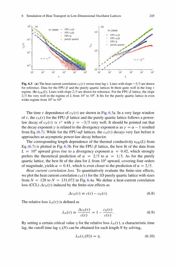
Fig. 6.3 (a) The heat current correlation cN .�/ versus time lag � . Lines with slope �3=5 are drawnfor reference. Data for the FPU-ˇ and the purely quartic lattices fit them quite well in the long �regime. (b) �GK.L/. Lines with slope 2=5 are drawn for reference. For the FPU-ˇ lattice, the slope2=5 fits very well in the regime of L from 103 to 106. It fits for the purely quartic lattice in evenwider regime from 102 to 106

The time � dependence of cN.�/ are shown in Fig. 6.3a. In a very large windowof � , the cN.�/ for the FPU-ˇ lattice and the purely quartic lattice follows a power-law decay of cN.�/ / � with D �3=5 very well. It should be pointed out thatthe decay exponent is related to the divergency exponent ˛ as D ˛ � 1 resultedfrom Eq. (6.7). While for the FPU-˛ˇ lattices, the cN.�/ decays very fast before itapproaches an asymptotic power-law decay behavior.

The corresponding length dependence of the thermal conductivity �GK.L/ fromEq. (6.7) is plotted in Fig. 6.3b. For the FPU-ˇ lattice, the best fit of the data fromL D 104 upward gives rise to a divergency exponent ˛ D 0:42, which stronglyprefers the theoretical prediction of ˛ D 2=5 to ˛ D 1=3. As for the purelyquartic lattice, the best fit of the data for L from 102 upward, covering four ordersof magnitude, yields ˛ D 0:41, which is even closer to the prediction of ˛ D 2=5.

Heat current correlation loss. To quantitatively evaluate the finite-size effects,we plot the heat current correlation cN.�/ for the 1D purely quartic lattice with sizesfrom N D 128 to N D 131;072 in Fig. 6.4a. We define a heat-current correlationloss (CCL) �cN.�/ induced by the finite-size effects as

�cN.�/ � c.�/ � cN.�/: (6.8)

The relative loss �N.�/ is defined as

�N.�/ � �cN.�/

c.�/D 1 � cN.�/

c.�/: (6.9)

By setting a certain critical value for the relative loss �N.�/, a characteristic timelag, the cutoff time lag �c.N/ can be obtained for each length N by solving,

�N.�c.N// D : (6.10)

246 L. Wang et al.

Fig. 6.4 (a) The heat currentcorrelation cN .�/ for thepurely quartic lattice forvarious lattice length N. Lineswith different slopes �2=3,�3=5 and �1=2, respectively,are drawn for reference. (b)�N.�/ as a function of � forvarious lattice length N.Oblique solid lines from thetop down stand for the fittingsof �N.�/, 3N�1:16�0:58, for Nranging from 128 to 4096.The horizontal dashed linerefers to �N.�/ D 0:1. �N.�/

cross this line at the cut offtime lag �c.N/. (c) The cutofftime lag �c.N/ as a functionof the lattice length N. Theblue dashed line stands forthe expectation in Eq. (6.13),2:84� 10�3N2

Since the asymptotic c.�/ can never be actually calculated, we thus need toapproximately replace c.�/ with cN.�/ for a finite long enough lattice instead.Under any existing criterion [31], the length of N D 131;072 is long enough forcorrelation times � � 5 � 104. Therefore, the asymptotic c.�/ refers to c131072.�/ inthe descriptions of our numerical simulations hereafter.

In Fig. 6.4b, the relative loss �N.�/ for the purely quartic lattice for various lengthN is plotted . The �N.�/ is larger in shorter lattices as one should expect. Interestingenough, all the data of �N.�/ as the correlation time � for various N fit the following

6 Simulation of Heat Transport in Low-Dimensional Oscillator Lattices 247

universal relation quite well:

�N.�/ � 3N�1:16�0:58: (6.11)

This relation implies that the cutoff time lag �c.N/ should follow a square-lawdependence on the lattice length N:

�c.N/ � .

3/

10:58 N2: (6.12)

For the critical value of D 0:1, namely, the cN.�/ decreases to 90% of the valueof c.�/ at � D �c.N/. The cutoff time lag �c.N/ as the function of length N can beobtained from Eq. (6.10) as

�c.N/ � 2:84 � 10�3N2: (6.13)

This is shown in Fig. 6.4c where good agreement with numerical data can beobserved.

It is reasonable to expect that Eq. (6.11) should also remain valid in larger Nregime. We are thus able to estimate the value of relative loss �N.�/ in Fig. 6.3a,which is no more than 10%. Given the fact that cN.�/ / � was fitted over fourorders of magnitude of � , the underestimate of ı induced therefrom must not behigher than j log10 0:9j=4 � 0:01. It is noticed that such an error is much smallerthan the difference between the three theoretical expectations D �2=3, D �3=5and D �1=2. The conclusion that c.�/ is best fitted as c.�/ / ��3=5 should notbe affected by this finite-size effect. We also expect that the cases in 2D [32] and3D [33] purely quartic lattices are also similar.

In summary, we have numerically calculated the length-dependent thermalconductivities � in a few typical 1D lattices by using both non-equilibrium heat bathand equilibrium Green-Kubo methods. Consistent results are obtained for thermalconductivity divergency exponent ˛. For the FPU-ˇ and the purely quartic lattices,the thermal conductivities � follows a power-law length-dependence of � / L0:4

very well, for a wide regime of L. While for the asymmetric FPU-˛ˇ lattices, largefinite-size effects are observed. As a result, � increases with lattice length veryslowly in a wide range of L. Our numerical simulations indicate that � regains itsincrease in yet longer length L [23, 26]. This is also consistent with some recentstudies [27, 28].

The studies of the heat current correlation loss in the purely quartic latticeindicate that for a not-very-large N, cN.�/ is close enough to the asymptotic c.�/within a very long correlation time � window. Therefore, we are able to extract�GK.L/ from Eq. (6.7) with an effective very long L by performing simulations in alattice with relatively much smaller size N, i.e. L D vs�c >> N. The research areaof the investigation of heat transport applicable for the Green-Kubo method is thusgreatly broadened [34].

248 L. Wang et al.

6.1.2 Logarithmic Divergent Thermal Conductivity in 2DMomentum-Conserving Nonlinear Lattices

For 2D and 3D momentum-conserving systems with higher dimensionality, con-sistent predictions are achieved from different theoretical approaches. The linearresponse approaches based on the renormalization group [6] and mode-couplingtheory [4, 35–37] both predict that the heat current autocorrelation function c.�/decays with the correlation time � as c.�/ / � , where D �1 and �3=2for 2D and 3D, respectively. These predictions indicate that the resulted thermalconductivity is logarithmically divergent as � / ln L in 2D systems and a finitevalue in 3D systems.

In 2D momentum-conserving systems, a logarithmic divergence of thermalconductivity of � / ln L is reported by numerical simulations in the FPU-ˇ latticewith rectangle [38, 39] and disk [40] geometries where vector displacements areconsidered. However, a power-law divergent thermal conductivity of � / L˛ is alsoobserved in the 2D FPU-ˇ lattices with scalar displacements [41].

In this subsection we systematically study the heat conduction in a few 2D squarelattices with a scalar displacement field ui;j, where the schematic 2D setup is plottedin Fig. 6.5a. The scalar 2D Hamiltonian reads

H DNXX

iD1

NYX

jD1Œp2i;j2

C V.ui;j � ui�1;j/C V.ui;j � ui;j�1/�; (6.14)

where NX and NY denotes the number of layers in X and Y directions. Theinter-particle potential takes the FPU form of V.u/ D 1

2k2u2 C 1

3k3u3 C 1

4k4u4.

Dimensionless units is applied and all the particle masses has been set to unity. Inorder to justify the logarithmic divergence and also study the influence of inter-particle coupling, we choose three types of lattices, i.e., the FPU-˛2ˇ lattice:k2 D k4 D 1, k3 D 2; the FPU-ˇ lattice: k2 D k4 D 1, k3 D 0; and the purelyquartic lattice: k2 D k3 D 0, k4 D 1.

The interaction forces between a particle labeled .i; j/ and its nearest right and upneighbors are f X

i;j D �dV.ui;j � ui�1;j/=dui;j and f Yi;j D �dV.ui;j � ui;j�1/=dui;j. The

local heat currents in the two directions are defined as jXi;j D 12.Pui;j C PuiC1;j/f X

iC1;j and

jYi;j D 12.Pui;j C Pui;jC1/f Y

i;jC1, respectively.

6.1.2.1 Non-equilibrium Heat Bath Method

We first calculate the thermal conductivity �NE in non-equilibrium stationary states.The fixed boundary conditions are applied in the X-direction, while periodicboundary conditions are applied in the Y-direction. The left- and right-most columnsare coupled to Langevin heat baths with temperatures TL D 1:5 and TR D 0:5,respectively, see Fig. 6.5a. Heat currents through the X-direction along with the

6 Simulation of Heat Transport in Low-Dimensional Oscillator Lattices 249

Fig. 6.5 (a) Scheme of a 2D square lattice. Heat current along the X axis is calculated.(b) Temperature profiles of different lattices. Curve groups from down top correspond to the FPU-˛2ˇ, FPU-ˇ, and purely quartic lattices, respectively. Only the data in the central region betweenthe two vertical dashed lines are taken into account in calculating the temperature gradient rT

direction of temperature gradient are measured. For each lattice with the largest size(2048� 64), the average heat current is performed over time period of 2 � 4 � 107in dimensionless units after long enough transient time. The temperature of eachcolumn is defined as the average temperature of all the particles in that column, i.e.,

T.i/ � 1

NY

NYX

jD1T.i; j/ D 1

NY

NYX

jD1hPu2i;ji;

The temperature profiles of different lattices for various NX � NY are plotted inFig. 6.5b. Those profiles with different sizes for the same lattice are all overlappedwith each other, which indicates that the temperature gradient rT along theX-direction can be well established. It is also confirmed that the temperatureprofiles and the heat currents along the lattices approach constant values whichare independent of the overall time used here. The thermal conductivity � for 2Dsystems is defined as:

�NE D � hJiNYrT

;

where J stands for the total heat current, and the temperature gradient rT is alongthe X direction. Since the lattice constant a is set to unity, the lattice length L is

250 L. Wang et al.

simply equivalent to the number of layers NX in X-direction. As shown in Fig. 6.5b,the shapes of temperature profiles are obviously nonlinear. Such a nonlinearityis caused by boundary effects rather than the intrinsic temperature dependenceof the thermal conductivity, as can be concluded by examining the temperaturedependence of �NE for different lattices in Fig. 6.6d. To reduce this boundary effect,the temperature gradient rT is calculated by a linear least-squares fitting of thetemperature profiles in the central region where the left- and right- most 1/4 of thelattices are excluded.

In Fig. 6.6a–c, the thermal conductivities �NE versus L with different widthsof NY are plotted in linear-log scales. In the large lattice size region, the narrowlattices with smaller NY posses higher values of thermal conductivities �NE. This isnot a surprise since the narrow 2D lattices are much closer to a 1D lattice wherehigh thermal conductivities are expected. The length dependence of �NE for the2D FPU-˛2ˇ lattice (Fig. 6.6a) with NY D 64 becomes flat, indicating that �NE

increases much more slowly than a logarithmic growing. In contrast, the thermalconductivities �NE for the 2D FPU-ˇ lattice diverges with length L more rapidly thana logarithmic divergence, as can seen from Fig. 6.6b and its inset. This is actually apower-law divergence of � / L˛ and the divergency exponent ˛ can be estimatedfrom the best fit of the last four points as ˛ D 0:27˙ 0:02. However, for 2D purely

Fig. 6.6 Thermal conductivity �NE in 2D (a) the FPU-˛ˇ, (b) the FPU-ˇ and (c) the purely quarticlattices versus lattice length L for various NY . The dashed line that indicate logarithmic growth isdrown for reference. Inset of (b): data for the FPU-ˇ lattice in double logarithmic scale. Solid linecorresponds to the power-law divergence L0:27. (d) �NE versus temperature T in various lattices

6 Simulation of Heat Transport in Low-Dimensional Oscillator Lattices 251

quartic lattices, the �NE displays a logarithmic growth as � / ln L over at least oneorder of magnitude in length scale, as in Fig. 6.6c.

6.1.2.2 Green-Kubo Method

Similar to the situation in 1D lattices [23], finite-size and finite-temperature-gradienteffects from the non-equilibrium heat bath method are considerable and not easyto be removed. We shall turn to the equilibrium Green-Kubo method [30] to seekhigher accuracy of numerical results.

In the Green-Kubo simulation, periodic boundary conditions are applied in boththe X- and Y-directions. The autocorrelation function of total heat current cX

NX ;NY.�/

in the X direction is defined as

cXNX ;NY

.�/ � 1

NXNYhJX.t/JX.t C �/it; (6.15)

where JX.t/ � Pi;j jXi;j.t/ is the instantaneous total heat current in the X-direction.

For simplicity, the subscripts NX and NY of cXNX ;NY

.�/ are omitted as cX.�/ hereafterexcept in case of necessity. The length-dependent thermal conductivity �GK.L/ fromthe Green-Kubo method can be defined as

�GK.L/ � 1

kBT2lim

NX!1 limNY !1

Z L=vs

0

cX.�/d�; (6.16)

where vs is again the speed of sound. Microcanonical simulations are performedwith zero total momentum [4] and specified energy density � which correspondsto the same temperature T D 1 for different lattices. The energy density � equals0.887, 0.892 and 0.75 for the 2D FPU-˛2ˇ, FPU-ˇ, and purely quartic lattices,respectively. A number of independent runs (64 for 1024 � 1024 and fewer forsmaller lattices) are carried out. Simulations of the largest lattices (1024�1024) areperformed for about total time of 107 in the dimensionless units.

The decays of cX.�/ with the correlation time � for different 2D lattices areplotted in Fig. 6.7a–c. To eliminate the finite-size effects, we have performedsimulations by varying NX and NY and only consider the asymptotic behavior whichis the part of curves overlapping with each other. Within the range of standard error,the satisfactory overlap with each other is clearly observed. In the specific caseswith NX D NY , the average of the autocorrelation function of ŒcX.�/ C cY.�/�=2

is plotted instead. This is equivalent to double the simulation time steps to achievehigher accuracy without actually performing any more computation. And due to thesymmetry of the square lattice, it is obvious to find that cX

512;1024.�/ D cY1024;512.�/,

where the simulations for the two lattices can be carried out in the same run.It is observed that in Fig. 6.7a, the cX.�/ in the 2D FPU-˛2ˇ lattices decays

much faster than the theoretical prediction of cX.�/ / ��1 in a wide regime ofcorrelation time .�/. As a result, the integrated �GK displays a saturation behavior

252 L. Wang et al.

Fig. 6.7 (a)–(c), cX.�/ for in NX � NY lattices. Lines correspond to ��1 are drawn for reference.(a) The FPU-˛2ˇ lattice. cX.�/ decays much faster than ��1 in short � regime. The decay tend toslow down for � > 300. (b) The FPU-ˇ lattice. cX.�/ decays obviously slower than ��1 in a quitewide regime of � . (c) The purely quartic lattice. cX.�/ follows ��1 very well in nearly three ordersof magnitude of � . (d)–(f), �GK.L/ in the X-direction in NX � NY lattices. (d) The FPU-˛2ˇ lattice.A flat �GK is again observed for L < 2000. Thereafter � tend to rise up. It is easy to understandthat slow down of the decay of c.�/ cannot instantly induce a visible rise up of �GK, since c.�/has already decayed to a too low value. (e) The FPU-ˇ lattice. In a wide regime of � , c� decaysobviously slower than ��1. Inset: data plotted in double logarithmic scale. Solid line correspondsto L0:25. (f) The purely quartic lattice. �GK for 1024 � 1024 follows the straight line very well innearly three orders of magnitude of � , This strongly supports a logarithmically divergent thermalconductivity. The slight rise for smaller lattices is due to the finite-size effect

with the length for large L in Fig. 6.7d. The rapid decay of cX.�/ tends to slowdown for yet longer time � . However, the asymptotic behavior cannot be numericallyconfirmed due to large fluctuations. In Fig. 6.7b, the cX.�/ in the 2D FPU-ˇ latticedecays evidently more slowly than ��1, which gives rise to a power-law divergenceof thermal conductivity of �GK / L˛ in Fig. 6.7e. The best fit of this divergencyexponent ˛ in the regime of L > 103 is obtained as ˛ D 0:25 ˙ 0:01. For the 2Dpurely quartic lattice as seen in Fig. 6.7c, the cX.�/ decays as the predicted behaviorof cX.�/ / ��1 for nearly three orders of magnitudes of correlation time � . Thisfinding strongly supports a logarithmic diverging thermal conductivity of � / ln L,which can be clearly observed in Fig. 6.7f. In all cases, the tendency of �GK fromGreen-Kubo method (shown in the right column of Fig. 6.7) is in good agreementwith that of �NE from non-equilibrium heat bath method (shown in Fig. 6.6).

6 Simulation of Heat Transport in Low-Dimensional Oscillator Lattices 253

In summary, we have extensively studied heat conduction in three 2D nonlinearlattices with both non-equilibrium heat bath method and Green-Kubo method. Theroles of harmonic and asymmetric terms of the inter-particle coupling are clearlyobserved by comparing the results for the purely quartic lattice and the other twolatices. In the 2D purely quartic lattice, the heat current autocorrelation function c.�/is found to decay as ��1 in three orders of magnitude from 101 to 104. This stronglysupports a logarithmically divergent thermal conductivity of � / ln L consistentwith the theoretical predictions. For the 2D FPU-ˇ lattice, our non-equilibriumand equilibrium calculations suggest a power-law divergence with a divergencyexponent˛ D 0:27˙0:02 and 0:25˙0:01, respectively. A very significant finite-sizeeffect which results a flat length dependence of �.L/ is observed in the 2D FPU-˛ˇlattice with asymmetric potential. Most existing numerical studies on 2D latticeswith asymmetric interaction terms suggest a logarithmically divergent behavior as� / ln L, e.g., the Fermi-Pasta-Ulam (FPU)-ˇ lattice with rectangle [38, 39] anddisk [40] geometries. It might be due to that the effect of the harmonic term is largelyoffset by that of the asymmetric term, thus yielding a logarithmic-like divergence ofthermal conductivity.

Similar to the findings of 1D lattices where � tends to diverge with length in thesame way in the thermodynamic limit for all kinds of lattices [23], it should also beexpected that � will diverge as log L in long enough 2D FPU-˛ˇ and FPU-ˇ latticesas already observed for 2D purely quartic lattice. However, in order to see suchan asymptotic divergence, 2D lattices with much larger sizes have to be simulatedwhich is beyond the scope of our current studies.

We should emphasize that such numerical studies are not only of theoreticalimportance. Progresses in nano-technology have made it possible to experimentallymeasure the size dependence of thermal conductivities in some 1D [42] and 2D [43–46] nano-scale materials.

6.1.3 Normal Heat Conduction in a 3DMomentum-Conserving Nonlinear Lattice

For 3D momentum-conserving systems, all the above-mentioned theories predictthat the heat current autocorrelation function decays with correlation time � as �

with D �3=2, which gives rise to a normal heat conduction. However, numericalsimulations are not so conclusive [47, 48]. It is only reported in 2008, by non-equilibrium simulations, that the running divergency exponent ˛L � d ln �=d ln Lof the 3D FPU-ˇ lattice shows a power law decay in L, thus vanishes in thethermodynamic limit [49]. Normal heat conduction in 3D systems is thereforeverified. However, according to the Green-Kubo formula, any power-law decay ofc.�/ / t with < �1will yield a finite value of thermal conductivity signaturing anormal heat conduction behavior [30]. In order to confirm the theoretical prediction

254 L. Wang et al.

of the specific value of D �3=2, the heat current autocorrelation function c.�/must be directly calculated by using the equilibrium Green-Kubo method.

We investigate the decay of the heat current autocorrelation function in a 3Dcubic lattice with a scalar displacement field ui;j;k. The 3D Hamiltonian reads

H DNXX

iD1

NYX

jD1

NZX

kD1

"p2i;j;k2

C V.ui;j;k � ui�1;j;k/

CV.ui;j;k � ui;j�1;k/C V.ui;j;k � ui;j;k�1/�; (6.17)

where V.u/ D 14u4 takes the purely quartic form. We choose this purely quartic

potential due to its simplicity and high nonlinearity, where close-to-asymptoticbehaviors can be achieved in shorter time and space scales. This model can alsobe regarded as the high temperature limit of the FPU-ˇ model. Periodic boundaryconditions, which provide the best convergence to thermodynamic limits, areapplied in all three directions, i.e., uNX ;j;k D u0;j;k, ui;NY ;k D ui;0;k and ui;j;NZ Dui;j;0. The interactions between a particle .i; j; k/ and its nearest neighbors are:f Xi;j;k D �dV.ui;j;k � ui�1;j;k/=dui;j;k, f Y

i;j;k D �dV.ui;j;k � ui;j�1;k/=dui;j;k and f Zi;j;k D

�dV.ui;j;k � ui;j;k�1/=dui;j;k. The local heat current in three directions are definedas jXi;j;k D 1

2.Pui;j;k C PuiC1;j;k/f X

iC1;j;k, jYi;j;k D 12.Pui;j;k C Pui;jC1;k/f Y

i;jC1;k, and jZi;j;k D12.Pui;j;kCPui;j;kC1/f Z

i;j;kC1, respectively. For convenience and simplicity, NX D NY D Wis always chosen and the focus is on the heat conduction in the Z direction withdifferent cross section area of W2 and length of NZ .

The heat current autocorrelation function cZ.�/ in the Z direction for a given Wis defined as [30]

cZ.�/ � limNZ!1

1

W2NZhJZ.t/JZ.t C �/it; (6.18)

where JZ.t/ � Pi;j;k jZi;j;k.t/ is the instantaneous total heat current in Z direction.

The length-dependent thermal conductivity �ZGK.L/ is defined as

�ZGK.L/ � 1

kBT2

Z L=vs

0

cZ.�/d�; (6.19)

where the constant vs is the speed of sound [4, 5]. vs is of order 1 for the presentlattice. Microcanonical simulations are performed with zero total momentum[4, 50,51] and fixed energy density � D 0:75which corresponds to the temperature T D 1.Due to the presence of statistical fluctuations, the simulation must be carried outlong enough, otherwise the real decay exponents of the autocorrelation functioncannot be determined with good enough accuracy. We perform the calculations by64-thread parallel computing. The simulation of the largest lattice (W D 64 andNZ D 128) is performed for the total time of 5 � 106 in dimensionless units.

6 Simulation of Heat Transport in Low-Dimensional Oscillator Lattices 255

Fig. 6.8 (a) cZ.�/ versus �for various NZ and W D 4

and 8. Lines with slopes �0:6and �1 are plotted forreference. (b) cZ.�/ versus �for various NZ and W D 16,32, and 64. Lines with slopes�1, �1:2, and �1:5 areplotted for reference. Thelarger the W, the longer thecurve follows the power lawdecay ��1:2, which suggeststhat c.�/ follows ��1:2 as Wis large enough.(c) Dependence of therunning exponent.�/ � d ln cZ.�/=d ln � onthe time lag � . Lines for D �0:6, �1, and �1:2 aredepicted for reference. Onecan see that for W � 16, thebottoms of the curves stopdecreasing and tend tosaturate at a W-independentvalue �1:2. The curves stayhere for a longer time as Wincreases

The decay of the autocorrelation function cZ.�/ with the correlation time � isplotted in Fig. 6.8a, b. For a given width W, we perform simulations by varying thelattice length NZ and consider only the asymptotic behavior shown in the part ofcurves overlapping with each other to avoid finite-size effects. In the short-timeregion, typically, for � < 101, all the curves of cZ.�/ are relatively flat. Thiscorresponds to the ballistic transport regime when � is shorter than or comparableto the phonon mean lifetime. Except in this ballistic regime, the cZ.�/ for W D 4

always decays more slowly than ��1, implying that the cross-section is too smallto display a genuine 3D behavior. The cZ.�/ for W D 8 decays faster than ��1 inthe regime � 2 .10; 30/, showing a weak 3D behavior. In longer time, the decayexponent becomes less negative and reverts to the exponent similar to that for thecase W D 4. For W D 16, the curves show a 3D behavior longer and finally againrevert to the 1D-like behavior. For width W D 32 and 64 where the similar reversalis expected, we fail to observe the 3D behavior in the asymptotic time limit due tothe presence of large statistical fluctuations. This picture indicates a crossover from

256 L. Wang et al.

3D to 1D behavior appearing at a W-dependent threshold for the correlation timeas �c.W/. Below this critical time �c, the system displays a 3D behavior, while a1D behavior is recovered above �c. In a macroscopic system, where the width andthe length are comparable, only 3D behaviors can be observed. This might be aconsequence of the universality of Fourier’s law in the macroscopic world in nature.

Furthermore, one can see that, for W 8, the larger the width, the longerthe cZ.�/ shows a power-law decay of ��1:2. This suggests that the asymptoticbehavior of the autocorrelation function should be cZ.�/ / ��1:2 when W islarge enough. It should be emphasized that the decay exponent is different fromthe traditional theoretical prediction of D �3=2. Interestingly, the numericallyobserved D �1:2 agrees with the formula D �2d=.2 C d/ (for d D 3) basedon the hydrodynamic equations for a normal fluid with an added thermal noise [6].However, in that paper the authors limit the validity of this formula to d � 2. Ourresult D �1:2 is also compatible with the value D �0:98 ˙ 0:25 for the 3DFPU model reported in [47].

In order to illustrate the 3D-1D crossover more clearly, we plot the �-dependenceof the running decay exponent .�/ defined as

.�/ � d ln cZ.�/

d ln �(6.20)

in Fig. 6.8c. For W D 4, the bottom of the running decay exponent .�/ is at �0:8,showing the absence of a 3D behavior. For W D 8, the bottom drops to about �1:1,showing a weak 3D behavior. For W 16, the bottoms of the .�/ tend to saturate ata W-independent value �1:2. As W increases, the .�/ stay at this value for a longertime. This indicates that D �1:2 is the asymptotic decay exponent for a “real” 3Dsystem. Since the decay exponent D �1 in 2D lattices, the threshold time �c.W/of the 3D-1D crossover can thus be reasonably defined as .�c.W// D �1. It can beestimated that �c.8/ � 35 and �c.16/ � 90. For W 32, it is hard to estimate thethreshold time due to large statistical errors.

The length-dependent thermal conductivity �ZGK.L/ for various W and NZ is

plotted in Fig. 6.9. similar to the 1D purely quartic lattice as shown in Fig. 6.8a,b, the 3D quartic lattice c.�/ can be correctly calculated for quite large correlationtime � by simulating a not-very-long lattice NZ , i.e. L D vs� >> NZ . We are thusable to evaluate �Z

GK.L/ for an effective length L, which is much longer than NZ . ForW D 4, the 3D behavior is nearly absent, similar to the picture shown in Fig. 6.8.As a result, the �Z

GK approaches to a 1D power-law divergence as L0:4 directly. ForW D 8, beyond trivial ballistic regime, the �Z

GK increases slowly at first, indicatingthe tendency to 3D behavior, and then inflects up to the 1D-like power-law behavior.For W D 16, the inflection occurs at a larger length L. Finally for W D 32 andW D 64, although the similar inflection is expected to occur at even larger length L,we are not able to see it due to numerical difficulties.

One can conclude that the 3D system should display normal heat conductionbehavior if the cross-section area W2 is large enough. Based on the thresholdcorrelation time �c.W/ defined earlier, a threshold length NZ

c .W/ can be defined

6 Simulation of Heat Transport in Low-Dimensional Oscillator Lattices 257

Fig. 6.9 �ZGK.L/ for various

W and NZ . For a given W,results for different values ofNZ are plotted in order todistinguish finite NZ effects.For each W we plot error barsonly for the data for thelongest NZ . One can see thetendency of the curves tobecome flat as W increases,indicating the presence ofnormal heat conduction.Dashed lines with slope 0.4are drawn for reference

accordingly by requiring NZc .W/ � vs�c.W/. The threshold length NZ

c .W/ deter-mined here is shorter than the estimation made by Saito and Dhar [49], in whicha lattice width W D 16 shows a 3D behavior up to L D 16384. In a recentexperimental study, an apparent 1D-like anomalous heat conduction behaviorappears in multiwall nanotubes with diameters around 10 nm and lengths of a few�m [42]. It seems that our estimation agrees with the experimental result. However,more detailed experimental measurements of heat conduction in shorter samples orsamples with larger cross-section of silicon nanowire [52, 53] or graphene [43], arenecessary to give an accurate estimation of the threshold length NZ

c .W/.A running exponent ˛.L/ is defined as the local slope of �Z

GK.L/ as

˛.L/ � d ln �ZGK.L/

d ln LD L

�ZGK.L/

cZ.�/: (6.21)

In the 3D regime, the cZ.�/ behaves as cZ.�/ � � as shown in Fig. 6.8. As L ! 1,the �Z

GK.L/ approaches a constant � since < �1. Then one can obtain

˛.L/ � L

�L D 1

�LC1: (6.22)

where ˛.L/ decays asymptotically as L�0:2 for D �1:2. This power-law decayof the exponent ˛.L/ with the length L as ˛.L/ / L�0:2 quantitatively explains theresult previously found in [49].

In summary, we have numerically studied heat conduction in 3D momentum-conserving nonlinear lattices by the Green-Kubo method. The main findings are:(1) For a fixed width W 8, a 3D-1D crossover was found to occur at a W-dependent threshold of a lattice size NZ

c .W/. Below NZc the system displays a 3D

behavior while it displays a 1D behavior above NZc . (2) In the 3D regime, the heat

258 L. Wang et al.

current autocorrelation function cZ.�/ decays asymptotically as � with D �1:2.This value being more negative than �1 indicates normal heat conduction, whichis consistent with the theoretical expectation. (3) The exponent D �1:2 impliesthat the running exponent ˛.L/ follows a power-law decay, ˛ / L�0:2, which alsoagrees very well with that reported in [49]. (4) The detailed value D �1:2 howeverdeviates significantly from the conventional theoretical expectation of D �1:5.

6.2 Simulation of Heat Transport with the Diffusion Method

In the numerical studies of heat transport in nonlinear lattices, the most fre-quently used methods are the direct non-equilibrium heat bath method [4] and theequilibrium Green-Kubo method [30]. For the non-equilibrium heat bath method,the system is connected with two heat baths in both ends and driven into astationary state. The averaged heat flux j is recorded which gives rise to the thermalconductivity � through the relation of j D ��rT. For the equilibrium Green-Kubomethod, the system is prepared from microcanonical dynamics without heat bath.The autocorrelation function CJJ.t/ of the total heat flux is recorded and the thermalconductivity � can be obtained by integrating CJJ.t/ via the Green-Kubo formula.

Besides the non-equilibrium heat bath method and Green-Kubo method, a noveldiffusion method is recently proposed by Zhao in studying the anomalous heattransport and diffusion processes of 1D nonlinear lattices [54]. This is also anequilibrium method, while the statistics can be drawn from microcanonical orcanonical dynamics. In contrast to the Green-Kubo method, this diffusion methodrelies on the information of the autocorrelation function of the local energy. InHamiltonian dynamics, the total energy is always a conserved quantity. Due tothis very property of energy conservation, it is then rigorously proved in a heatdiffusion theory recently developed by Liu et al, stating that the energy diffusionmethod is equivalent to the Green-Kubo method in the sense of determining thesystem’s thermal conductivity [55]. In particular, the energy diffusion method isable to provide more information than that from the Green-Kubo method. The real-time spatiotemporal excess energy density distribution �E.x; t/ plays the role of agenerating function which is essential for the analysis of underlying heat conductionbehavior.

In principle, the thermal conductivity � can be generally expressed in a length-dependent form as � / L˛ with L the system length. For system with normalheat conduction, the heat divergency exponent ˛ D 0 implies that � is length-independent obeying the Fourier’s heat conduction law. The heat divergencyexponent ˛ D 1 represents a ballistic heat conduction behavior. For 0 < ˛ < 1,the system displays the so-called anomalous heat conduction behavior. On theother hand, the Mean Square Displacement (MSD) h�x2.t/iE of the excess energygenerally grows with time asymptotically as h�x2.t/iE / tˇ where the energydiffusion exponent ˇ classifies the diffusion behaviors. The ˇ D 1 and 2 represent

6 Simulation of Heat Transport in Low-Dimensional Oscillator Lattices 259

the normal and ballistic energy diffusion behaviors, respectively. For 1 < ˇ < 2,the diffusion process is called superdiffusion.

In 1D nonlinear lattice systems, the heat conduction and energy diffusionoriginating from the same energy transport process are closely related. What is therelation between the heat conduction and energy diffusion processes? The relationformula between heat divergency and energy diffusion exponents ˛ D ˇ � 1 isproposed by Cipriani et al. by investigating single particle Levy walk diffusionprocess [56]. This same formula is then formally derived as a natural result fromthe heat diffusion theory [55]. This relation formula tells that: (1) Normal energydiffusion with ˇ D 1 corresponds to normal heat conduction with ˛ D 0 andvice versa. This is the case for 1D 4 lattice and Frenkel-Kontorova lattice [54].(2) Ballistic energy diffusion with ˇ D 2 implies ballistic heat conduction with˛ D 1 and vice versa. The 1D Harmonic lattice and Toda lattice fall into thisclass [54]. (3) Superdiffusive energy diffusion with 1 < ˇ < 2 yields anomalousheat conduction with 0 < ˛ < 1 and vice versa. The 1D FPU-ˇ lattice is verified toposses energy superdiffusion with ˇ D 1:40 and anomalous heat conduction with˛ D 0:40 [54, 57] belonging to this class.

Besides total energy, total momentum is another conserved quantity for 1Dnonlinear lattices without on-site potential, such as the FPU-ˇ lattice. It is com-monly believed that the conservation of momentum is essential for the actual heatconduction behavior. Predictions from mode coupling theory [4] and renormal-ization group theory [6] claim that momentum conservation should give rise toanomalous heat conduction in one dimensional systems. However, there is oneexception to these predictions: the 1D coupled rotator lattice, which displays normalheat conduction behavior despite its momentum conserving nature [22, 58]. Thisunusual phenomenon stimulates the efforts to explore the interplay between energytransport and momentum transport. The transport coefficient corresponding to themomentum transport is the bulk viscosity. For momentum conserving system, inprinciple, there should also be a formal connection between the momentum transportand the momentum diffusion. This very momentum diffusion theory has also beendeveloped for 1D momentum-conserving lattices [59]. Due to the complexity ofbulk viscosity, the momentum diffusion theory is more complicated than the heatdiffusion theory. Nevertheless, there seems to be a relation between the actualbehaviors of energy and momentum transport implied from extensive numericalstudies.

In the following, the energy diffusion method will be first introduced. Theheat diffusion theory will be derived in the framework of linear response theory.Numerical simulations for two typical 1D nonlinear lattices will be used to verifythe validity of this heat diffusion theory. Some results from the energy diffusionmethod will be shown for typical 1D lattices. The momentum diffusion method willthen be discussed. The momentum diffusion theory will be derived in the same senseas heat diffusion theory for the 1D lattice systems. Some numerical results from themomentum diffusion method will be displayed and potential connection betweenmomentum and heat transports will be discussed in the final part.

260 L. Wang et al.

6.2.1 Energy Diffusion

In this part, we first introduce the energy diffusion method in the investigation forenergy diffusion process of 1D lattices. The heat diffusion theory will be derived inthe linear response regime and verified by numerical simulations. Some numericalresults from this energy diffusion method will be presented to demonstrate theadvantages of this novel method.

6.2.1.1 Heat Diffusion Theory

The heat diffusion theory [55, 59] unifies energy diffusion and heat conduction in arigorous way. The central result reads

d2h�x2.t/iE

dt2D 2CJJ.t/

kBT2cv; (6.23)

where kB is the Boltzmann constant and cv is the volumetric specific heat. Theautocorrelation of total heat flux CJJ.t/ on the right hand side is the term entering theGreen-Kubo formula from which thermal conductivity can be calculated. The MSDh�x2.t/iE of energy diffusion describes the relaxation process in which an initiallynonequilibrium energy distribution evolves towards equilibrium:

h�x2.t/iE �Z.x � hxiE/

2�E.x; t/dx D hx2.t/iE � hxi2E : (6.24)

This normalized fraction of excess energy �E.x; t/ at a certain position x at time treads

�E.x; t/ D ıhh.x; t/ineq

ıED ıhh.x; t/ineqR

ıhh.x; 0/ineqdx: (6.25)

Here the excess energy distribution is proportional to the deviation ıhh.x; t/ineq �hh.x; t/ineq � hh.x/ieq, where h�ineq denotes the expectation value in the nonequi-librium diffusion process, h�ieq denotes the equilibrium average, and h.x; t/ denotesthe local Hamiltonian density. For isolated energy-conserving systems, this totalexcess energy, ıE D R

ıhh.x; t/ineqdx remains conserved. Therefore, the normalizedcondition

R�E.x; t/dx D 1 is fulfilled during the time evolution as a result of energy

conservation.In the linear response regime, the deviation of local excess energy can be

explicitly derived in terms of equilibrium spatiotemporal correlation Chh.x; tI x0; 0/of local Hamiltonian density h.x; t/ as

ıhh.x; t/ineq D 1

kBT

ZChh.x; tI x0; 0/.x0/dx0; (6.26)

6 Simulation of Heat Transport in Low-Dimensional Oscillator Lattices 261

where Chh.x; tI x0; t0/ � h�h.x; t/�h.x0; t0/ieq, with �h.x; t/ D h.x; t/ � hh.x/ieq,and the �.x/h.x/ represents a small perturbation switched off suddenly at timet D 0, with .x/ 1.

Therefore, the normalized excess energy distribution can be derived fromEqs. (6.25) and (6.26) as

�E.x; t/ D 1

N

ZChh.x � x0; t/.x0/dx0; (6.27)

where N D kBT2cvR.x/dx is the normalization constant.

The key point which connects energy diffusion and heat conduction is the localenergy continuity equation due to energy conservation

@h.x; t/

@tC @j.x; t/

@xD 0; (6.28)

where j.x; t/ is the local heat flux density. One can then obtain

@2Chh.x; t/

@t2D @2Cjj.x; t/

@x2; (6.29)

By defining the total heat flux JL D R L=2�L=2 j.x; t/dx and the autocorrelation function

of total heat flux CJJ.t/ � limL!1hJL.t/JL.0/ieq=L D R 1�1 Cjj.x; t/dx, the central

result (6.23) of the heat diffusion theory can be derived.As a result of energy conservation, the heat diffusion theory of Eq. (6.23) gives

the general relation between energy diffusion and heat conduction. The actualbehavior of energy diffusion or heat conduction can be normal or anomalous whilethe relation (6.23) remains to be the same:

1. For normal energy diffusion, the MSD increases asymptotically linearly withtime, i.e.

h�x2.t/iE Š 2DEt; (6.30)

in the infinite time limit t ! 1. Here DE is the so-called thermal diffusivity.According to Eq. (6.23), the corresponding thermal conductivity � can beobtained as

� DZ 1

0

CJJ.t/

kBT2dt D cv

2lim

t!1dh�x2.t/iE

dtD cvDE: (6.31)

This is nothing but the Green-Kubo expression for normal heat conduction.2. For ballistic energy diffusion, the MSD is asymptotically proportional to the

square of time as

h�x2.t/iE / t2: (6.32)

262 L. Wang et al.

Substituting this expression into Eq. (6.23), one can deduce that CJJ.t/ is a non-decaying constant, reflecting the ballistic nature of heat conduction as well.

3. For superdiffusive energy diffusion, the MSD obeys

h�x2.t/iE / tˇ; 1 < ˇ < 2: (6.33)

From Eq. (6.23), the decay of CJJ.t/ is a slow process as CJJ.t/ / tˇ�2 andthe integral of CJJ.t/ diverges. In this situation, no finite superdiffusive thermalconductivity exists. The typical way in practice is to introduce an upper cutofftime ts � L=vs with vs the speed of sound due to renormalized phonons [60].A length-dependent superdiffusive thermal conductivity can be obtained throughEq. (6.23):

� � 1

kBT2

Z L=vs

0

CJJ.t/dt D cv

2

dh�x2.t/iE

dt

ˇ̌ˇ̌t�L=vs

/ Lˇ�1: (6.34)

The length-dependent anomalous thermal conductivity is usually expressed as� / L˛ . One can immediately obtain the scaling relation between energydiffusion and heat conduction

˛ D ˇ � 1; (6.35)

which is a general relation and not limited to superdiffusive energy diffusiononly.

4. For subdiffusive energy diffusion, the MSD follows asymptotically

h�x2.t/iE / tˇ; 0 < ˇ < 1: (6.36)

From the relation in (6.23), the autocorrelation function of total heat flux readsasymptotically

CJJ.t/ / ˇ.ˇ � 1/tˇ�2: (6.37)

The CJJ.t/ remains integrable and the thermal conductivity can be derived as

� DZ 1

0

CJJ.t/

kBT2dt D cv

2lim

t!1dh�x2.t/iE

dt� lim

t!1 tˇ�1 D 0: (6.38)

This vanishing integral of CJJ.t/ is not surprising, if one notices that theasymptotic prefactor of CJJ.t/ in (6.37) is a negative value due to ˇ � 1 < 0.

6 Simulation of Heat Transport in Low-Dimensional Oscillator Lattices 263

6.2.1.2 Numerical Verification of the Heat Diffusion Theory

The heat diffusion theory of Eq. (6.23) developed for continuous system is generaland applicable also for discrete system. We choose two typical 1D nonlinear latticesto demonstrate the validity of this heat diffusion theory. One is the purely quarticFPU-ˇ (qFPU-ˇ) lattice which is the high temperature limit of FPU-ˇ lattice, whereenergy diffusion is superdiffusive and heat conduction is anomalous or length-dependent [18, 23]. The dimensionless Hamiltonian with finite N D 2M C 1 atomsreads

H DX

i

Hi DX

i

�1

2p2i C 1

4.uiC1 � ui/

4

�; (6.39)

where pi and ui denote momentum and displacement from equilibrium position fori-th atom, respectively. The index i is numerated from �M to M.

The other one is the 4 lattice which shows normal energy diffusion as well asnormal heat conduction [54, 61, 62]. The dimensionless Hamiltonian reads

H DX

i

Hi DX

i

�1

2p2i C 1

2.uiC1 � ui/

2 C 1

4u4i

�: (6.40)

In the numerical simulations, we adopt the microcanonical dynamics whereenergy density E per atom is set as the input parameter. Algorithm with higheraccuracy of fourth-order symplectic method [63, 64] can be used to integrate theequations of motions. Periodic boundary conditions ui D uiCN and pi D piCN areapplied and the equilibrium temperature T can be calculated from the definition T DTi D hp2i i, where h�i denotes time average which equals to the ensemble averagedue to the chaotic and ergodic nature of these two nonlinear lattices. The volumetricspecific heat need to be calculated via the relation cv D .hH2

i i � hHii2/=T2 whichis independent of the choice of index i. For qFPU-ˇ lattice, the volumetric specificheat cv D 0:75 is a temperature-independent constant.

In order to define the discrete expression of excess energy density distribution�E.i; t/, we first introduce the energy-energy correlation function, reading:

CE.i; tI j; t D 0/ � h�Hi.t/�Hj.0/ikBT2cv

; (6.41)

where �Hi.t/ � Hi.t/ � hHi.t/i. Applying a localized, small initial excess energyperturbation at the central site, .i/ D "ıi;0 in Eq. (6.27), the discrete excess energydistribution can be obtained:

�E.i; t/ DX

j

CE.i; tI j; 0/. j/=" D CE.i; t W j D 0; t D 0/; �M � i � M: (6.42)

264 L. Wang et al.

The MSD h�x2.t/iE of energy diffusion of Eq. (6.24) for discrete lattice can bedefined as

h�x2.t/iE �X

i

i2�E.i; t/ DX

i

i2CE.i; tI j D 0; t D 0/; �M � i � M; (6.43)

by noticing that hx.t/iE D 0.The second derivative of h�x2.t/iE can be numerically obtained as

d2h�x2.t/iE

dt2� h�x2.t C�t/iE � 2h�x2.t/iE C h�x2.t ��t/iE

.�t/2(6.44)

where �t is the time difference between two consecutive recorded h�x2.t/iE. Theautocorrelation function of total heat flux CJJ.t/ for discrete lattice system is definedas CJJ.t/ D h�J.t/�J.0/i=N, with J.t/ D P

i ji.t/. The local heat flux ji.t/ D�Pui@V.ui � ui�1/=@ui is derived from local energy continuity equation where V.x/denotes the form of potential energy in Hamiltonian.

In Fig. 6.10, we verify the main relation (6.23) for 1D qFPU-ˇ lattice. The MSDof energy diffusion h�x2.t/iE as the function of time is plotted in Fig. 6.10a. Its

Fig. 6.10 Numerical verification of the main relation of Eq. (6.23) of heat diffusion theory for1D qFPU-ˇ lattice. (a) The MSD h�x2.t/iE of energy diffusion as the function of time t in log-log scale. (b) The second derivative of MSD d2h�x2.t/iE=dt2 (hollow circles) and the rescaledautocorrelation function of total heat flux 2CJJ.t/=.T2cv/ (solid line) as the function of time t inlog-log scale. The perfect agreement between them demonstrates the validity of the main relationof Eq. (6.23). The Boltzmann constant kB has been set as unity when applying dimensionless unitsin numerical simulations. The simulations are performed for a qFPU-ˇ lattice with the averageenergy density per atom E D 0:015 and the number of atoms N D 601

6 Simulation of Heat Transport in Low-Dimensional Oscillator Lattices 265

Fig. 6.11 Numerical verification of the main relation of Eq. (6.23) of heat diffusion theory for1D 4 lattice. (a) and (b): the MSD h�x2.t/iE of energy diffusion as the function of time tfor 0 < t < 10 and 10 < t < 200, respectively. (c) and (d): the second derivative ofMSD d2h�x2.t/iE=dt2 (hollow circles) and the rescaled autocorrelation function of total heat flux2CJJ.t/=.T2cv/ (solid line) as the function of time t in linear-linear scale for 0 < t < 10 and log-linear scale for 10 < t < 200, respectively. The perfect agreement between them demonstrates thevalidity of the main relation of Eq. (6.23). The simulations are performed for a 4 lattice with theaverage energy density per atom E D 0:4 and the number of atoms N D 501

second derivative d2h�x2.t/iE=dt2 is extracted out and directly compared with therescaled autocorrelation function of total heat flux 2CJJ.t/=.kBT2cv/ in Fig. 6.10b.The perfect agreement between them justifies the validity of the main relation (6.23)predicted from heat diffusion theory. The numerical results for 1D 4 latticeare also plotted in Fig. 6.11 and same conclusion can be obtained. It should bepointed out that the 1D qFPU-ˇ lattice displays superdiffusive energy diffusion andanomalous heat conduction, while 1D 4 lattice shows normal energy diffusion andheat conduction. These facts can be observed by noticing that the autocorrelationfunction CJJ.t/ eventually follows a power law decay as CJJ.t/ / t�0:60 for qFPU-ˇlattice and an exponential decay as CJJ.t/ / e�t=� for 4 lattice where � representsa characteristic relaxation time.

6.2.1.3 Energy Diffusion Properties for Typical 1D Lattices

The heat diffusion theory formally connects the energy diffusion and heat con-duction as described in Eq. (6.23). It enables us to use energy diffusion methodto investigate the heat conduction process. More importantly, the energy diffusionmethod is able to provide more information about the heat transport process thanthe Green-Kubo method or the direct non-equilibrium heat bath method.

266 L. Wang et al.

The key information from the energy diffusion method is the spatiotemporaldistribution of excess energy �E.i; t/, from which the MSD of energy diffusionh�x2.t/iE can be generated. The second derivative of h�x2.t/iE gives rise to theautocorrelation function of total heat flux CJJ.t/ which finally yields the thermalconductivity via Green-Kubo formula. With the knowledge of �E.i; t/, one canresolve the expression of h�x2.t/iE or CJJ.t/, but not vice versa. Therefore, indetermining the actual heat conduction behavior, the excess energy distribution�E.i; t/ plays the essential role of a generating function.

To illustrate the importance [59]: the coupled rotator lattice

H DX

i

�1

2p2i C .1 � cos .uiC1 � ui//

�; (6.45)

and the amended coupled rotator lattice

H DX

i

�1

2p2i C .1 � cos .uiC1 � ui//C K

2.uiC1 � ui/

2

�; (6.46)

where an additional quadratic interaction potential term is added.The excess energy distributions �E.i; t/ for coupled rotator lattice are plotted in

Fig. 6.12a. For sufficiently large times, the excess energy distribution �E.i; t/ evolves

Fig. 6.12 Energy diffusion processes in the 1D coupled rotator lattice. (a) Spatial distribution ofthe energy autocorrelation �E.i; t/ D CE.i; tI j D 0; t D 0/. The correlation times are t D 200; 400

and 600 from top to the bottom in the central part, respectively. The distribution of �E.i; t/ follows

the Gaussian normal distribution as �E.i; t/ � 1p

4�DEte�

i24DE t . (b) The MSD of the energy diffusion

h�x2.t/iE as the function of time. The solid straight line is the best fit for the MSD h�x2.t/iE

implying a normal diffusion process. The simulations are performed for a coupled rotator latticewith the average energy density per atom E D 0:45 and the number of atoms N D 1501

6 Simulation of Heat Transport in Low-Dimensional Oscillator Lattices 267

very closely into a Gaussian distribution function with its profile perfectly given by

�E.i; t/ � 1p4�DEt

e� i24DEt ; (6.47)

where DE denotes the diffusion constant for energy diffusion. As a result, the MSDof energy diffusion h�x2.t/iE depicts at a linear time dependence

h�x2.t/iE �X

i

i2�E.i; t/ DX

i

i21p4�DEt

e� i24DEt D 2DEt; (6.48)

for sufficiently long time as can be seen in Fig. 6.12b, being the hall mark for normaldiffusion. Accordingly, heat diffusion theory for normal energy diffusion impliesthat the heat conduction behavior is normal as well, with the thermal conductivitygiven by � D cvDE.

This normal energy diffusion behavior also occurs for other 1D lattice systemswith normal heat conduction, such as 4 lattice and Frenkel-Kontorova lattice [54].

For the 1D amended coupled rotator lattice described in Eq. (6.46), the excessenergy distributions �E.i; t/ are plotted in Fig. 6.13a. Besides the central peak, thereare also two side peaks moving outside with a constant sound velocity vs. It isamazing that this excess energy distribution �E.i; t/ of 1D nonlinear lattice closely

Fig. 6.13 Energy diffusion processes in the 1D amended coupled rotator lattice. (a) Spatialdistribution of the energy autocorrelation �E.i; t/ D CE.i; tI j D 0; t D 0/. The correlation timesare t D 200; 600 and 1000 from top to the bottom in the central part, respectively. Besides thecentral peak, there are two side peaks moving outside with the constant sound velocity. This isthe Levy walk distribution giving rise to a superdiffusive energy diffusion. (b) The MSD of theenergy diffusion h�x2.t/iE as the function of time. The solid straight line is the best fit for thesuperdiffusive MSD as h�x2.t/iE / t1:40. The simulations are performed for an amended coupledrotator lattice with the average energy density per atom E D 1. The number of atoms N D 2501

and K D 0:5

268 L. Wang et al.

resembles to the single particle Levy walk distribution �LW.x; t/ [56]

�LW.x; t/ /

8ˆ̂̂<

ˆ̂̂:

t�1=� exp .�ax2

t2=�/; jxj . t1=�

tx���1; t1=� < jxj < vtt1��; jxj D vt0; jxj > vt

(6.49)

where a is an unknown constant and v is the particle velocity. This Levy walk dis-tribution �LW.x; t/ is a result of a particle moving ballistically between consecutivecollisions with a waiting time distribution .t/ / t���1 and a velocity distributionf .u/ D Œı.u � v/C ı.u C v/�=2.

The MSD for the Levy walk distribution �LW.x; t/ follows a time dependenceof h�x2.t/iLW / tˇ with ˇ D 3 � �. In Fig. 6.13b, the time dependence of MSDh�x2.t/iE of energy diffusion for the 1D amended coupled rotator lattice is plottedwhere the best fit indicates that ˇ D 1:40. This will in turn correspond to a� D 1:60

in the Levy walk scenario. According to the relation formula of Eq. (6.35) of heatdiffusion theory, the corresponding heat conduction should be anomalous with adivergent length dependent thermal conductivity of � / L˛ with ˛ D 0:40 [23].

It is very interesting to notice that there is a characteristic � for the Levy walkdistribution. By requiring that the heights of the central peak and side peaks decaywith a same rate in the Levy walk distribution (6.49), one can obtain �1=� D 1��which gives rise to the golden ratio � D .

p5 C 1/=2 � 1:618. As a result, the

corresponding characteristic energy superdiffusion exponent ˇ D .5 � p5/=2 �

1:382 and the anomalous heat conduction exponent ˛ D .3 � p5/=2 � 0:382 can

be derived. Interesting enough, Lee-Dadswell et al. derived the same exponent ˛ D.3 � p

5/=2 as the converging value of a Fibonacci sequence in a toy model withinthe framework of hydrodynamical theory in 2005 [65]. Actually, this exponent isnot far from the existing numerical results [18, 23, 66].

6.2.2 Momentum Diffusion

In the following part, the momentum diffusion method will be introduced formomentum conserving systems. A momentum diffusion theory will be derivedin the same sense as heat diffusion theory. The numerical results reflecting themomentum diffusion properties will then be presented for several 1D nonlinearlattices. Based on the numerical results, the possible connection between momentumand energy transports will be discussed in the final part.

6 Simulation of Heat Transport in Low-Dimensional Oscillator Lattices 269

6.2.2.1 Momentum Diffusion Theory

In analogy to the heat diffusion, one can also construct a momentum diffusiontheory [59] for lattice systems which reads:

d2h�x2.t/iP

dt2D 2

kBTCJP.t/; (6.50)

where h�x2.t/iP denotes the momentum diffusion and CJP.t/ is the centeredautocorrelation function of total momentum flux.

The MSD of excess momentum h�x2.t/iP can be defined as

h�x2.t/iP DX

i

i2�P.i; t/; �M � i � M: (6.51)

The excess momentum distribution �P.i; t/ describes the nonequilibrium relaxationprocess of momentum due to a small kick of short duration to the j-th atom. Thekick occurs with a constant impulse I, yielding a force kick at site j as fj.t/ D Iı.t/.The normalized �P.i; t/ is given by

�P.i; t/ D hpi.t/irePihpi.t/ire

; (6.52)

where hpi.t/ire represents the response of momentum of i-th atom to the smallperturbation of �fj.t/uj. In the linear response regime, it can be obtained thathpi.t/ire D ICP.i; tI j; 0/, where

CP.i; tI j; 0/ D h�pi.t/�pj.0/ikBT

(6.53)

is the autocorrelation function for the excess momentum fluctuation. The sumPi CP.i; tI j; 0/ D 1 at time t D 0 and remains normalized due to the conservation

of momentum. As a result, the excess momentum distribution �P.i; t/ assumes theform

�P.i; t/ D CP.i; tI j D 0; t D 0/; (6.54)

if the kick is put at the atom with index j D 0.The centered autocorrelation function of momentum flux CJP.t/ in Eq. (6.50) is

given by

CJP.t/ D 1

Nh�JP.t/�JP.0/i; JP D

X

i

jPi ; (6.55)

270 L. Wang et al.

where the local momentum flux jPi D �@V.ui � ui�1/=@ui with V.x/ the form ofinteraction potential is obtained from the discrete momentum continuity relation

dpi

dt� jPi C jPiC1 D 0: (6.56)

It should be emphasized that here the momentum flux �JP.t/, unlike for energyflux, cannot be replaced with JP.t/ itself. This is so because the equilibrium averageis typically non-vanishing with hJP.t/i D N�, where � denotes a possibly non-vanishing internal equilibrium pressure in cases where the interaction potential isnot symmetric.

The transport coefficient of momentum conduction related to the momentumdiffusion is the bulk viscosity . However, the presence of a finite, isothermal soundspeed vs implies that here the momentum spread contains a ballistic componentwhich should be subtracted [67, 68] to yield the effective bulk viscosity :

� 1

kBT

Z 1

0

CJP.t/dt � 1

2v2s t: (6.57)

In case that the momentum diffusion occurs normal, one can invoke the concept ofa finite momentum diffusivity

DP � 1

2lim

t!1

�dh�x2.t/iP

dt� v2s t

�: (6.58)

Therefore, for the discrete lattices, this effective bulk viscosity precisely equalsthe momentum diffusivity times the atom mass m (set to unity in the dimensionlessunits), namely

D DP: (6.59)

If the excess momentum density spreads not normally, the limit in Eq. (6.58) nolonger exits. The integration in Eq. (6.57) formally diverges, thus leading to aninfinite effective bulk viscosity.

In the practice, it is found that the finite effective bulk viscosity and normal heatconduction always emerge in pair, so does the infinite effective bulk viscosity andanomalous heat conduction. This constitutes an alternative implementation of theinvestigation of heat conduction behavior in lattice systems.

6.2.2.2 Momentum Diffusion Properties for Typical 1D Lattices

The momentum diffusion theory connects the momentum diffusion and momentumtransport via Eqs. (6.50) and (6.57). Similar to what we have discussed for the

6 Simulation of Heat Transport in Low-Dimensional Oscillator Lattices 271

Fig. 6.14 Momentum diffusion processes in the 1D coupled rotator lattice. (a) Spatial distributionof the energy autocorrelation �P.i; t/ D CP.i; tI j D 0; t D 0/. The correlation times aret D 200; 400 and 600 from top to the bottom in the central part, respectively. The distribution

of �P.i; t/ follows the Gaussian normal distribution as �P.i; t/ � 1p

4�DPte�

i24DPt . (b) The MSD of

the momentum diffusion h�x2.t/iP as the function of time. The solid straight line is the best fitfor the MSD h�x2.t/iP implying a normal diffusion process. The simulations are performed fora coupled rotator lattice with the average energy density per atom E D 0:45 and the number ofatoms N D 1501

energy diffusion, the excess momentum distribution �P.i; t/ is the most importantinformation we need to gather for momentum diffusion method.

We still consider the 1D coupled rotator lattice of Eq. (6.45) and amendedcoupled rotator lattice of Eq. (6.46) [59]. In Fig. 6.14a, the excess momentumdistributions �P.i; t/ for different correlation times t D 200; 400 and 600 are plotted.At sufficiently large times, the distributions �P.i; t/ follow the Gaussian distributionas

�P.i; t/ � 1p4�DPt

e� i24DPt ; (6.60)

where DP represents the momentum diffusion constant. The MSD h�x2.t/iP ofmomentum diffusion thus grows linearly with time at large times, i.e. h�x2.t/iP �2DPt, as can be seen from Fig. 6.14. There is no ballistic component for thedistributions �P.i; t/ in 1D coupled rotator lattice. Accordingly, the finite effectivebulk viscosity can be simply obtained as D DP. This result is consistent with thefact that the 1D coupled rotator lattice displays normal heat conduction behavior.

For the 1D amended coupled rotator lattice, the energy diffusion is superdiffusiveand its heat conduction is anomalous. The excess momentum distributions �P.i; t/for different correlation times at t D 200; 600 and 1000 are plotted in Fig. 6.15a.In contrast to the coupled rotator lattice, here only two side peaks moving outsidewith a constant sound velocity vs exist. To evaluate the true behavior of momentumconduction, this ballistic component within the momentum diffusion should be

272 L. Wang et al.

Fig. 6.15 Momentum diffusion processes in the 1D amended coupled rotator lattice. (a) Spatialdistribution of the energy autocorrelation �P.i; t/ D CP.i; tI j D 0; t D 0/. The correlation timesare t D 200; 600 and 1000 from top to the bottom, respectively. There is no central peak and twoside peaks moves outside with the constant sound velocity vs. (b) The self-diffusion of the side peakof the momentum spreading. The rescaled side peaks tı�P.i; t/ of four different correlation timesat t D 400; 600; 800 and 1000 all collapse into the same curve in the center of the rescaled movingframe .i�vst/=tı with a scaling exponent ı D 0:55. The scaling exponent ı D 0:55 > 0:50 impliesthe self-diffusion is superdiffusive and the effective bulk viscosity is infinite. The simulations areperformed for an amended coupled rotator lattice with the average energy density per atom E D 1.The number of atoms N D 2501 and K D 0:5

subtracted. One should instead analyze the self-diffusion behavior of the side peaksof the distributions �P.i; t/. In Fig. 6.15b, the rescaled side peaks tı�P.i; t/ as thefunction of rescaled position of the peak center .i � vst/=tı are plotted for fourdifferent correlation times at t D 400; 600; 800 and 1000. With the choice ofı D 0:55, the rescaled distributions collapse into a single curve all together. Thisrescaling behavior with ı D 0:55 implies a superdiffusive self-diffusion for the sidepeaks, while normal self-diffusion would require for ı D 0:50.

The integration of Eq. (6.57) is then divergent, giving rise to an infinite effectivebulk viscosity . This infinite is consistent with the finding that the heat conductionis anomalous, since the energy diffusion is superdiffusive as can be observed inFig. 6.13b. From our perspective and our own numerical results, the infinite bulkviscosity and divergent length-dependent thermal conductivity always emerge inpair. However, there are some other numerical results and approximate theoriesindicating that finite bulk viscosity and anomalous heat conduction might coexistfor symmetric lattices such as FPU-ˇ lattice [65, 69]. This is still an open issue anddeserves more investigation in the future.

In summary, a novel diffusion method is introduced to investigate the heattransport in 1D nonlinear lattices. The heat and momentum diffusion theoriesformally relate the diffusion processes to their corresponding conduction processes.The properties of energy and momentum diffusions for typical 1D lattices are

6 Simulation of Heat Transport in Low-Dimensional Oscillator Lattices 273

presented and more fundamental information about transport processes can beprovided from this novel method.

Acknowledgements This work is supported by the National Natural Science Foundation of Chinaunder Grant No. 11275267(L.W.), Nos. 11334007 and 11205114 (N.L.), the Fundamental ResearchFunds for the Central Universities, and the Research Funds of Renmin University of China15XNLQ03 (L.W.), the Program for New Century Excellent Talents of the Ministry of Educationof China with Grant No. NCET-12-0409 (N.L.), the Shanghai Rising-Star Program with grantNo. 13QA1403600 (N.L.). Computational resources were provided by the Physical Laboratory ofHigh Performance Computing at Renmin University of China(L.W.) and Shanghai SupercomputerCenter (N.L.).

References

1. James, M.L., Smith, G.M., Wolford, J.C.: Applied Numerical Methods for Digital Computa-tion. HarperCollins College Publishers, New York (1993)

2. Dormand, J.R., El-Mikkawy, M.E.A., Prince, P.J.: IMA J. Numer. Anal. 7, 423 (1987)3. Dormand, J.R., El-Mikkawy, M.E.A., Prince, P.J.: IMA J. Numer. Anal. 11, 297 (1991)4. Lepri, S., Livi, R., Politi, A.: Phys. Rep. 377, 1 (2003)5. Dhar, A.: Adv. Phys. 57(5), 457 (2008)6. Narayan, O., Ramaswamy, S.: Phys. Rev. Lett. 89, 200601 (2002)7. Mai, T., Narayan, O.: Phys. Rev. E 73, 061202 (2006)8. Wang, J.S., Li, B.: Phys. Rev. Lett. 92, 074302 (2004)9. Wang, J.S., Li, B.: Phys. Rev. E 70, 021204 (2004)

10. Delfini, L., Lepri, S., Livi, R., Politi, A.: Phys. Rev. E 73, 060201 (2006)11. Delfini, L., Lepri, S., Livi, R., Politi, A.: J. Stat. Mech. Theory Exp. 2007(02), P02007 (2007)12. Delfini, L., Denisov, S., Lepri, S., Livi, R., Mohanty, P.K., Politi, A.: Eur. Phys. J. Special

Topics 146, 21 (2007)13. Santhosh, G., Kumar, D.: Phys. Rev. E 77, 011113 (2008)14. Liu, S., Liu, J., Hänggi, P., Wu, C., Li, B.: Phys. Rev. B 90, 174304 (2014)15. Pereverzev, A.: Phys. Rev. E 68, 056124 (2003)16. Lukkarinen, J., Spohn, H.: Commun. Pure Appl. Math. 61(12), 1753 (2008)17. Lepri, S., Livi, R., Politi, A.: Phys. Rev. Lett. 78(10), 1896 (1997)18. Mai, T., Dhar, A., Narayan, O.: Phys. Rev. Lett. 98(18), 184301 (2007)19. Delfini, L., Lepri, S., Livi, R., Politi, A.: Phys. Rev. Lett. 100, 199401 (2008)20. Dhar, A., Narayan, O.: Phys. Rev. Lett. 100, 199402 (2008)21. Prosen, T., Campbell, D.K.: Phys. Rev. Lett. 84, 2857 (2000)22. Gendelman, O.V., Savin, A.V.: Phys. Rev. Lett. 84(11), 2381 (2000)23. Wang, L., Wang, T.: Europhys. Lett. 93, 54002 (2011)24. Delfini, L., Lepri, S., Livi, R., Mejia-Monasterio, C., Politi, A.: J. Phys. A Math. Theor. 43(14),

145001 (2010)25. Zhong, Y., Zhang, Y., Wang, J., Zhao, H.: Phys. Rev. E 85, 060102 (2012)26. Wang, L., Hu, B., Li, B.: Phys. Rev. E 88, 052112 (2013)27. Savin, A.V., Kosevich, Y.A.: Phys. Rev. E 89, 032102 (2014)28. Das, S.G., Dhar, A., Narayan, O.: J. Stat. Phys 154, 204 (2014)29. Chen, S., Wang, J., Casati, G., Benenti, G.: Phys. Rev. E 90, 032134 (2014)30. Kubo, R., Toda, M., Hashitsume, N.: Statistical Physics II. Springer Series in Solid State

Sciences, vol. 31. Springer, Berlin (1991)31. Chen, S., Zhang, Y., Wang, J., Zhao, H.: Phys. Rev. E 89, 022111 (2014)32. Wang, L., Hu, B., Li, B.: Phys. Rev. E 86, 040101 (2012)

274 L. Wang et al.

33. Wang, L., He, D., Hu, B.: Phys. Rev. Lett. 105, 160601 (2010)34. Wang, L., Xu, L., Zhao, H.: Phys. Rev. E 91, 012110 (2015)35. Ernst, M.H., Hauge, E.H., van Leeuwen, J.M.J.: Phys. Rev. A 4, 2055 (1971)36. Ernst, M., Hauge, E., van Leeuwen, J.: J. Stat. Phys. 15(1), 7 (1976)37. Ernst, M., Hauge, E., van Leeuwen, J.: J. Stat. Phys. 15(1), 23 (1976)38. Lippi, A., Livi, R.: J. Stat. Phys. 100, 1147 (2000)39. Yang, L., Grassberger, P., Hu, B.: Phys. Rev. E 74, 062101 (2006)40. Xiong, D., Wang, J., Zhang, Y., Zhao, H.: Phys. Rev. E 82, 030101 (2010)41. Grassberger, P., Yang, L.: eprint arXiv:cond-mat/020424742. Chang, C.W., Okawa, D., Garcia, H., Majumdar, A., Zettl, A.: Phys. Rev. Lett. 101, 075903

(2008)43. Ghosh, S., Bao, W., Nika, D.L., Subrina, S., Pokatilov, E.P., Lau, C.N., Balandin, A.A.: Nat.

Mater. 9, 555 (2010)44. Xu, X., Wang, Y., Zhang, K., Zhao, X., Bae, S., Heinrich, M., Tinh Bui C., Xie, R., Thong,

J.T.L., Hong, B.H., Loh, K.P., Li, B., Oezyilmaz, B.: eprint arXiv:1012.293745. Wang, Z., Xie, R., Bui, C.T., Liu, D., Ni, X., Li, B., Thong, J.T.L.: Nano Lett. 11, 113 (2011)46. Nika, D.L., Askerov, A.S., Balandin, A.A.: Nano Lett. 12, 3238 (2012)47. Shiba, H., Yukawa, S., Ito, N.: J. Phys. Soc. Jpn. 75(10), 103001 (2006)48. Shiba, H., Ito, N.: J. Phys. Soc. Jpn. 77(5), 054006 (2008)49. Saito, K., Dhar, A.: Phys. Rev. Lett. 104, 040601 (2010)50. Lepri, S., Livi, R., Politi, A.: Europhys. Lett. 43, 271 (1998)51. Lepri, S., Livi, R., Politi, A.: Phys. Rev. E 68, 067102 (2003)52. Morales, A.M., Lieber, C.M.: Science 279(5348), 208 (1998)53. Ma, D.D.D., Lee, C.S., Au, F.C.K., Tong, S.Y., Lee, S.T.: Science 299(5614), 1874 (2003)54. Zhao, H.: Phys. Rev. Lett. 96, 140602 (2006)55. Liu, S., Hänggi, P., Li, N., Ren, J., Li, B.: Phys. Rev. Lett. 112, 040601 (2014)56. Cipriani, P., Denisov, S., Politi, A.: Phys. Rev. Lett. 94, 244301 (2005)57. Wang, L., Wu, Z., Xu, L.: Phys. Rev. E 91, 062130 (2015)58. Giardinà, C., Livi, R., Politi, A., Vassalli, M.: Phys. Rev. Lett. 84, 2144 (2000)59. Li, Y., Liu, S., Li, N., Hänggi, P., Li, B.: New J. Phys. 17, 043064 (2015)60. Li, N., Li, B., Flach, S.: Phys. Rev. Lett. 105, 054102 (2010)61. Hu, B., Li, B., Zhao, H.: Phys. Rev. E 61, 3828 (2000)62. Aoki, K., Kusnezov, D.: Phys. Lett. A 265(4), 250 (2000)63. Skokos, C., Krimer, D.O., Komineas, S., Flach, S.: Phys. Rev. E 79, 056211 (2009)64. Laskar, J., Robutel, P.: Celest. Mech. Dyn. Astron. 80(1), 39 (2001)65. Lee-Dadswell, G.R., Nickel, B.G., Gray, C.G.: Phys. Rev. E 72, 031202 (2005)66. Zhao, H., Wen, Z., Zhang, Y., Zheng, D.: Phys. Rev. Lett. 94, 025507 (2005)67. Helfand, E.: Phys. Rev. 119, 1 (1960)68. Resibois, P., de Leener, M.: Classical Kinetic Theory of Fluids. Wiley,

New York/London/Sidney/Toronto (1977)69. Spohn, H.: J. Stat. Phys. 154, 1191 (2014)