Embed Size (px)
Citation preview

134
CHAPTER 6
SEGMENTATION OF EXUDATES
Like hemorrhages, exudates are also the pathological features in
DR. The segmentation of exudates also greatly helps in automatic screening
system. The exudates are precipitations of plasma protein in the retinal region
and appear as bright, reflective, white or cream-colored lesions on the retinal
image. The exudates are a developed stage from microaneurysms and
hemorrhages. The vision loss is inevitable, if it is ignored.
The segmentation of the exudates is carried out using various
clustering techniques and the results are presented and discussed elaborately
in this chapter. The images from the standard database are used for testing,
validating and measure the performance of the proposed technique. The
relative merits of each clustering technique have been presented.
The segmentation of exudates will be successful only when the OD
is eliminated from the retinal image as it has more or less equal brightness.
Detection of the OD center and OD boundary using vessel-direction matched
filter and masking of OD have been explained in the Chapter 4. In this
process, the images with OD detection and elimination by masking
techniques are used as input images. OD masked image is subjected to further
processing to segment the exudates. As exudates are the bright region,
Hussain et al (2010) and Giancardo et al (2011) applied the thresholding
technique to segment the exudates.

135
In th
resh
oldi
ng te
chni
que,
the
thre
shol
d va
lue
of th
e im
age
is s
et a
s
one
or m
ore
than
one
. If
thre
shol
d va
lue
is s
et a
s on
e, t
he i
mag
e w
ill b
e
divi
ded
into
two
regi
ons
as e
xpla
ined
in C
hapt
er 4
, Sec
tion
4.1.
2. I
n re
tinal
imag
es,
the
thre
shol
d va
lues
can
not
be f
ixed
eas
ily a
s th
ey h
ave
diff
eren
t
inte
nsity
lev
els.
Furth
er,
it w
ill n
ot b
e un
iform
. H
ence
, th
e th
resh
oldi
ng
tech
niqu
e is
not
abl
e to
yie
ld s
atis
fact
ory
resu
lts.
In o
rder
to
achi
eve
the
segm
enta
tion
proc
ess s
ucce
ssfu
lly, v
ario
us c
lust
erin
g te
chni
ques
like
Fuz
zy C
Mea
ns
(FC
M),
K
mea
ns
clus
terin
g,
com
bina
tion
of
K
mea
ns
with
mor
phol
ogy
and
fuzz
y ar
e us
ed i
n se
gmen
tatio
n pr
oces
s. Th
e pr
opos
ed
clus
terin
g te
chni
ques
are
app
lied
over
the
OD
mas
ked
imag
es a
fter c
onve
rting
them
into
gra
y sc
ale
imag
es. T
he e
ntire
pro
cess
is s
chem
atic
ally
illu
stra
ted
as
bloc
k di
agra
m in
Fig
ure
6.1.
Figu
re 6
.1 B
lock
dia
gram
for
exud
ates
segm
enta
tion
OD
mas
ked
Retin
al Im
age
RG
B to
gra
y K m
eans
and
m
orph
olog
y Fu
zzy
C M
eans
Fu
zzy
Exud
ates
Seg
men
tatio
n an
d Pa
ram
etric
Mea
sure
s
Km
eans

136
6.1
CL
UST
ER
ING
TE
CH
NIQ
UE
S
The
clus
terin
g te
chni
que
uses
int
ensi
ty r
elat
ions
hip
amon
g th
e pi
xels
of
an i
mag
e. I
t cla
ssifi
es th
e pi
xels
int
o di
ffer
ent g
roup
s ba
sed
on it
s in
tens
ity. I
n a
parti
cula
r gr
oup,
sim
ilarit
y m
easu
rem
ents
am
ong
the
pixe
ls a
re
carr
ied
out a
nd d
epen
ding
on
thei
r val
ue, t
he p
ixel
s will
be
clus
tere
d. A
mon
g th
e va
rious
clu
ster
s, th
e si
mila
rity
leve
l w
ill b
e va
ryin
g w
here
as i
n th
e pa
rticu
lar
clus
ter
the
sim
ilarit
y va
lue
will
be
mor
e or
less
the
sam
e w
ithou
t m
uch
varia
tion.
A s
tand
ard
proc
edur
e fo
r as
sign
ing
a pi
xel
to th
e cl
uste
r is
ba
sed
on th
e m
ean
valu
e of
the
pixe
ls p
rese
nt in
the
clus
ter.
Ach
ievi
ng s
uch
a gr
oupi
ng r
equi
res
a si
mila
rity
met
ric th
at in
volv
es th
e in
put
vect
ors
and
its
valu
e re
flect
s the
ir si
mila
rity
Jeya
ram
an (2
012)
.
In o
rder
to
achi
eve
bette
r re
sult,
the
RG
B c
olor
im
ages
are
co
nver
ted
into
gra
y sc
ale
imag
es a
nd re
duce
d in
to 2
56 X
256
siz
e be
fore
the
appl
icat
ion
of th
e cl
uste
ring
tech
niqu
e. T
his
proc
ess
will
ena
ble
one
to o
btai
n re
sults
in
a sh
ort
time
as t
hese
pro
cess
es a
re i
tera
tive
ones
. C
onve
rsio
n of
R
GB
col
or s
pace
to g
ray
scal
e is
exp
lain
ed in
Cha
pter
4, S
ectio
n 4.
1.1.
1. T
he
vario
us c
lust
erin
g te
chni
ques
are
dis
cuss
ed i
n th
e fo
llow
ing
sect
ions
in
a se
quen
tial m
anne
r.
6.2
FUZ
ZY
C M
EA
NS
CL
UST
ER
ING
(FC
M)
It is
a d
ata
clus
terin
g al
gorit
hm a
nd it
clu
ster
s th
e pi
xel b
ased
on
its
mem
bers
hip
grad
e in
to d
iffer
ent c
lust
ers.
The
vario
us s
teps
inv
olve
d in
this

137
(a)
(b)
(c)
(d)

138
The images with various clusters contain useful information based
on their grouping. From the above resultant image, the first cluster shows the
exudates clearly compared with the other clusters as the intensity level of the
exudates matches with the first cluster. In most of the tested images, the
exudates are segmented in first cluster only. However, it is not necessary that
in all the images the exudates will be segmented in the first cluster. The
segmentation process basically depends on the intensity of the exudates
corresponding to the clusters. In other clusters, the features like blood vessels
and optic disc are also segmented. The 1st cluster image is considered as the
segmented output of exudates. The algorithm is tested with images of STARE
database and the parametric measures are carried out. The results are
presented in Table 6.1 with image identification number, TP, FP, FN, TN, SE,
SPE, ACC and processing time in seconds.
Table 6.1 Parametric measures of the fuzzy c means method
FUZZY C MEANS Sl.No. Image ID Number of Pixels Percentage Time
(Sec.)TP FP FN TN SE SPE ACC1 im0017 24708 3076 8543 387173 74 99 97 03.642 im0049 14317 2158 8864 398161 62 99 97 06.603 im0052 5278 95047 2617 320558 67 77 77 09.704 im0064 24606 1290 11321 386283 68 100 97 06.975 im0096 6325 1079 1958 414138 76 100 99 10.596 im0106 3195 5619 2305 412381 58 99 98 11.557 im0124 2598 25279 1738 393885 60 94 94 10.168 im0171 60053 1426 9843 352178 86 100 97 11.829 im0172 35949 1131 5657 380763 86 100 98 12.19
10 im0176 50755 1970 14357 356418 78 99 96 08.7711 im0178 29297 2084 17760 374359 62 99 95 10.7712 im0227 8012 22016 819 392653 91 95 95 11.6413 im0246 49912 3331 18491 351766 73 99 95 06.2314 im0308 66604 1478 19631 335787 77 100 95 12.6915 im0313 27137 516 12085 383762 69 100 97 09.17
Mean value 73 97 95 09.50

139
From the results, it is inferred that the mean values of SE, SPE,
ACC and time in seconds are estimated as 73%, 97%, 95% and 9.5 sec
respectively. The FCM method has the highest specificity of 97% and
accuracy of 95%. However, the sensitivity is relatively lower as 73%. Hence,
it is attempted to increase the sensitivity using various other algorithms. In
continuation of this algorithm, K means clustering technique is adopted and
the various steps involved are briefed in the next section.
6.3 K MEANS CLUSTERING ALGORITHM
It is one of the clustering techniques that classify a given data set to
a certain fixed number of clusters based on the similarity of the pixels or
group of pixels. The fixed number of clusters is assumed as ‘K’. Unlike in the
previous technique, membership grade of the pixel is not considered in this
algorithm. Instead, it classifies each pixel in a group with the closest mean
distance between the centroid and the pixel. It is an iterative procedure and
this algorithm clusters the data iteratively by computing a mean intensity for
each group and the various steps involved in this algorithm are given below.
Step 1 : Provide the input data and number of clusters
Step 2 : Calculate the cluster centroids based on assumed initial
value
Step 3 : Calculate the distance of each pixel from class centroid
Step 4 : Group pixels into k clusters based on minimal distance
from centroids
Step 5 : Calculate new centroid for each cluster
Step 6 : Classify into groups based on new centroid and distance
Step 7 : Test if any centroid changes its position.

140
Step 8 : If there are changes repeat step 3- 8, else go to step 9
Step 9 : End
The above steps are illustrated as a flow diagram in Figure 6.3.
Figure 6.3 Flow chart for K means clustering technique
In this method, if there are ‘K’ number of clusters, the number of
centroids or cluster centers are also ‘K’ corresponding to each cluster. The
centroid for a cluster is based on the range of intensity values present in a
particular cluster. Usually, it is assumed as the mean value of the variation
range corresponding to the intensity levels. At the beginning stage, these
centroids are fixed at suitable positions and they are iterated towards the exact
location in the process.
No
Yes
Number of Cluster K Number of Cluster K
Start
End
Distance between the objects and Centroids
Centroid
Grouping Based on minimum distance
Object Move to the
Group
Number of Cluster K

141
The pixels present in the original image are transferred to different clusters based on their intensity value. This algorithm predicts a cluster center in each group so that a cost function (objective function) of dissimilarity (distance) measure is minimized. Euclidean distance is a measure of distance between the pixel intensity and the cluster center. It is used for calculating the error function. The equation for error function in terms of euclidean distance for the pixels contained in cluster is given in Equation (6.1). Finally, this algorithm aims at minimizing a squared error objective function (J).
2)(
1 1j
ji
k
j
n
i
cxJ (6.1)
where,
2)(j
ji cx - Euclidean distance measure between a data point
‘ ix ’belonging to cluster j and its cluster centre ‘ jc ’.
If a pixel has a value corresponding to the nearest value of the centroid of the particular cluster, it is transferred to that cluster. This process continues till all the pixels are grouped into any one of the clusters that are assumed to be initial clusters. Further, the centroids of the clusters are iterated towards the better values within the cluster. The above step is repeated until no pixel is moving from one cluster to another. When the step reaches this point, if the clusters are stable, the clustering process stops.
Usually, exudates are the high intensity pixel regions in the retinal image. Based on this property, this clustering technique is applied to segment the exudates in the retinal images. OD masked image is adopted for the K means clustering algorithm and is separated into five clusters based on the intensities in the image. Resultant clusters after the application of the K means clustering on STARE database image with an identification number im0049 are shown in Figures.6.4 (a) to (f). Figures 6.4 (a),(b),(c),(d) and (e) show the resultant images of five different clusters with various intensity levels.

142
(a) (b)
(c) (d)
(e) (f)
Figure 6.4 Resultant output of K means clustering technique (a) output of cluster1 (b) output of cluster 2 (c) output of cluster 3 (d) output of cluster 4 (e) output of cluster 5 (f) post processed output

143
The resultant images of the clusters shown in Figures 6.4 (d) and
(e) have segmented the exudates in comparison with other clusters. However,
Figure 6.4 (d) has segmented even small exudates compared to Figure 6.4 (e).
As a result, Figure 6.4 (d) is suitable for further processing to fill the image
regions and holes (contour of bright pixels contained darker region within the
boundary). The filling of the holes is achieved by filling bright pixels in the
holes.
The image with holes filled is shown in Figure 6.4 (f) and the
image with the segmented exudates is considered as output using K means
clustering technique. Similar to FCM, K means clustering algorithm is
implemented in the exudates images in the STARE database and the predicted
SE , SPE, ACC and the processing time of are tabulated in Table 6.2.
Table 6.2 Parametric measures of the K means clustering method
K MEANS Sl.No. Image ID Number of Pixels Percentage Time
(Sec.)TP FP FN TN SE SPE ACC1 im0017 28884 8878 4367 381371 87 98 97 1.77 2 im0049 15090 4001 5091 399318 75 99 98 1.78 3 im0052 6181 435 1314 415570 82 100 100 2.82 4 im0064 33447 20776 2480 366797 93 95 95 3.33 5 im0096 6745 1675 1538 413542 81 100 99 3.85 6 im0106 7188 19456 707 396149 91 95 95 3.02 7 im0124 2666 50172 72 370590 97 88 88 3.07 8 im0171 65132 5256 4764 348348 93 99 98 3.07 9 im0172 40671 13883 935 368011 98 96 97 3.00
10 im0176 61949 48929 3163 309459 95 86 88 3.04 11 im0178 43070 18860 3987 357583 92 95 95 3.16 12 im0227 6440 2758 2391 411911 73 99 99 3.09 13 im0246 64426 60502 3977 294595 94 83 85 3.07 14 im0308 76597 8224 9638 329041 89 98 96 3.12 15 im0313 33735 7711 5487 376567 86 98 97 2.60
Mean value 88 95 95 2.92

144
In this clustering technique, the mean values of the parametric
measures are 88%, 95%, 95% and 2.92 sec corresponding to SE, SPE, ACC
and the processing time respectively. It is to be noticed that the SE has
increased from 73% to 88% with the marginal loss of SPE from 97% to 95%
whereas the accuracy remains the same in comparison with the previous
technique. Further, in view of improving the above parametric measures,
efforts have been taken with other post-processing operations like
morphology that is briefed in the following section.
6.4 COMBINATION OF K MEANS AND MORPHOLOGY
The resultant image from the previous section after application of
K means clustering is taken for morphological operations to enhance the
sensitivity. In morphological operations, the segmented pixels are dilated
using structuring elements to acquire the other smaller left out details in the
cluster. The considered structuring elements are with parameters as length 3
and angle 900 and 00. The parameter ‘Length’ is the distance between the
centers of the structuring element members at opposite ends of the line, and
the angle of the line is measured in a counterclockwise direction from the
horizontal axis. The above two structuring elements are applied for dilation
one after another. The steps involved in the morphological operations are
detailed in Chapter 3 Section 3.4. The resultant image after the dilation
is shown in Figure 6.5. (a). Further, the holes are filled as explained in
the previous section to obtain better segmentation and this is shown in
Figure 6.5 (b).

145
(a) (b)Figure 6.5 Post processed K means clustered image (a) Dilated image
using structuring elements (b) The post processed image with holes filled
The combination of K means and morphological operations is
performed on the images available in STARE database. The parametric
measures are performed and the results are presented in Table 6.3.
Table 6.3 Parametric measures of the combination of K means and
morphology method
K MEANS AND MORPHOLOGY Sl. No. Image ID Number of Pixels Percentage Time
(Sec.) TP FP FN TN SE SPE ACC1 im0017 31726 19351 1525 370898 95 95 95 2.77 2 im0049 21270 13870 1911 386449 92 97 96 3.30 3 im0052 6867 1252 628 414753 92 100 100 2.85 4 im0064 34968 31372 959 356201 97 92 92 3.04 5 im0096 7654 5443 629 409774 92 99 99 2.81 6 im0106 7889 50983 6 364622 100 88 88 2.59 7 im0124 2738 61052 0 359710 100 85 86 2.83 8 im0171 66534 8619 3362 344985 95 98 97 2.91 9 im0172 40995 13779 611 368115 99 96 97 3.33 10 im0176 63643 58444 1469 299944 98 84 86 3.88 11 im0178 46281 33101 776 343342 98 91 92 2.77 12 im0227 8615 130543 216 284126 98 69 69 2.64 13 im0246 67148 66966 1255 288131 98 81 84 2.60 14 im0308 78824 11178 7411 326087 91 97 96 2.91 15 im0313 35062 15291 4160 368987 89 96 95 3.12
Mean value 96 91 91 2.96

146
The mean values of the parametric measures of SE, SPE, ACC and
the processing time are 96%, 91%, 91% and 2.92 sec respectively. It is to be
noted that the SE has increased in comparison with the previous two
algorithms as 96% as against 73% and 88%. On the other hand, the specificity
is higher in the FCM as 97% and it gradually decreases in K means algorithm
as 95% and in the present algorithm as 91%. It is because in dilation
operation the nearby pixels are associated with the exudates that reduce the
specificity. With regard to ACC, both the previous algorithms of FCM and K
means have 95% and the present algorithm yields 91%. This is also due to the
reason mentioned above. The computational time for the FCM is
comparatively higher as 9.50 seconds and it is more or less the same as 2.92
and 2.96 for the later algorithms. It is general expectation that the
segmentation algorithm should have higher specificity and accuracy and the
search process is extended for other techniques so as to improve the above
parameters.
In the above algorithms, the intensity levels of the pixels are
divided into five clusters and the pixel with a particular value just below or
above the prescribed centroid of the cluster is grouped into the clusters
accordingly. This approach is based on the crisp value of the pixels, whereas
in the fuzzy logic, the membership function is used to group the pixels based
on the membership value corresponding to intensity. Hence, there is a
possibility of improving the parametric measures of the segmentation process
using fuzzy logic. The Fuzzy Inference System (FIS) is applied to achieve the
above expectation and the steps involved are discussed in the next section.
6.5 FUZZY INFERENCE SYSTEM
In this technique, the pixels are grouped based on the membership
function corresponding to intensity values. The various important

147
terminologies used in the Fuzzy logic like Fuzzy Set (FS), Fuzzy membership
functions (FMF) and Fuzzy Rules (FR) are briefed below.
Fuzzy Set : If ‘S’ is a collection of objects, then ‘x’ in the fuzzy set
‘FS’ is the set of defined elements.
FS = {(x, mf (x)) x S} (6.2)
where, ‘mf (x)’ is the membership function of ‘x’ in ‘S’ which varies from 0
to 1.
The fuzzy inference system consists of five different steps that are
detailed below with its functioning.
Step 1: Define the inputs and outputs for the fuzzy inference
system: The input and output set of variables are predetermined and are
called as fuzzy variables. The fuzzy value of the pixel is determined with the
rules framed using the above input and output set of variables. The range of
all possible values of fuzzy variables is called universe of discourse.
Step 2: Set up fuzzy membership functions for input: Fuzzification
is the process of converting crisp values into fuzzy values. Membership
functions are used to determine the selected value and its grouping and its
value varies from 0 to 1. There are different shapes of membership
functions: triangular, trapezoidal, Gaussian and bell-shaped etc. In this
present work, triangular membership function is used. Based on this
function, the input crisp values are converted into fuzzy values.
Step 3: Set up fuzzy membership functions for the output: It is
developed in a similar way as discussed in Step 2 for the set of output values
also.

148
Step 4: Create a fuzzy rule base: The rules are framed so as to
obtain the desired output. The set of input and output fuzzy variables are used
to frame the rules in the form of IF-THEN statements. The membership
values are used to select the rules to predict the output. The membership
function and rules are adjusted to achieve the desired performance.
Step 5: Set of membership values for fuzzy outputs are reconverted
to crisp output so as to use the image for further application, and this process
is called defuzzification. The popular defuzzification methods are center of
gravity method, average of maxima method and midpoint of maxima method.
In this process for defuzzification, the centroid method is adopted.
Based on the above steps, two types of fuzzy models proposed by
Mamdani and Sugeno Jang et al (1997) are used by various researchers in
different image processing systems. The models developed by them have a
flexibility to select the number of input and output variables, set of rules and
various types of membership functions. In the present work, the model
proposed by Mamdani is considered in the segmentation process of exudates.
The model consists of a fuzzifier, fuzzy rule base, an inference engine and a
defuzzifier.
The above stages are coded in MATLAB environment and the
different fuzzy logic tool boxes available in the software are used for the
segmentation process. The Fuzzy Logic Toolbox is a collection of builtin
functions in MATLAB. It provides tools to create and edit fuzzy inference
systems within the framework of MATLAB. There are five primary
Graphical User Interface (GUI) tools for building, editing and observing
fuzzy inference systems. In the fuzzy logic toolbox, namely the fuzzy
inference system or FIS editor, the membership function editor, the rule
editor, the rule viewer and the surface viewer are available in the software.

149
6.5.1 Fuzzy Clustering for Exudates Segmentation
Fuzzy model proposed by Mamdani is used to segment the
exudates. OD masked image is used as an input for fuzzy system. Input color
image is converted into gray scale image. The gray scale image is adopted for
segmenting the exudates. The initial step is to fuzzify the inputs to be
achieved by triangular membership function. The concept of the triangular
function with its lower limit ‘a’ and upper limit ‘b’ and a value ‘m’,
where a < m < b is shown in Figure 6.6. The equation for predicting the
membership value xA of the corresponding input value of the ‘x’ is given
in Equation (6.3).
Figure 6.6 Triangular membership function
bx
bxmmbxb
mxaamax
ax
xA
,0
,
,
,0
(6.3)
Input x
Mem
bers
hip
valu
e

150
The input gray values are in the range of 0 to 255. The entire range
is fuzzified by five overlapped MFs such as mf1, mf2, mf3, mf4 and mf5. The
input gray scale value is divided into five groups using five membership
functions as shown below in the format as
MF='mf1':'trimf',[a m b].
MF1 = 'mf1':'trimf',[-94.5 8.12 80.25]
MF2 = 'mf2':'trimf',[26.8 85.7 152.72]
MF3 = 'mf3':'trimf',[132 189 249.57]
MF4 = 'mf4':'trimf',[78.2 134 204.87]
MF5 = 'mf5':'trimf',[197 252.95 281]
The above five membership functions in the range of 0 to 255 are
shown graphically representing ‘a’, ‘m’ and ‘b’ on x – axis and degree of
membership values that ranges from 0 to 1 on y-axis as shown in Figure 6.7.
For the particular input value of ‘x’, it is possible to predict membership value
using the triangular function.
0 50 100 150 200 250
0
0.2
0.4
0.6
0.8
1
Gray values
mf1 mf2 mf3mf4 mf5
Figure 6.7 Fuzzified input using the triangular membership function

151
In the similar way, the triangular membership function is used for
output set of variables. It is divided into five ranges not necessarily equal such
as mf1, mf2, mf3, mf4 and mf5 using the triangular membership functions as
shown in Figures 6.8 (a) to (e). The range of gray scale value is divided into
five groups and assigned as output variables as shown below in the format
similar to the input membership function.
output1 = 'mf1':'trimf', [-102 0 50.46]
output2 = 'mf2':'trimf', [53.2 80.25 107]
output3 = 'mf3':'trimf', [101.25 130 149]
output4 = 'mf4':'trimf', [150 173.71 201]
output5 = 'mf5':'trimf', [197 223.15 251]
Figures 6.8 (a), (b), (c), (d) and (e) show the triangular membership
function of the output1, output2, output3, output4 and output 5.
0 50 100 150 200 250
0
0.2
0.4
0.6
0.8
1
Gray values
mf1
output 1
0 50 100 150 200 250
0
0.2
0.4
0.6
0.8
1
Gray values
mf2
output 2
(a) (b)
Figure 6.8 Membership functions for output variables

152
0 50 100 150 200 250
0
0.2
0.4
0.6
0.8
1
Gray values
mf3
output 3
0 50 100 150 200 250
0
0.2
0.4
0.6
0.8
1
Gray values
mf4
output 4
(c) (d)
0 50 100 150 200 250
0
0.2
0.4
0.6
0.8
1
Gray values
mf5
output 5
(e)
Figure 6.8 (Continued)
Further, fuzzy rules are framed and executed. Rules for the
proposed fuzzy system are given in Table 6.4. These rules are created in the
Mamdani fuzzy models available in the MATLAB.

153
Table 6.4 Rules for the fuzzy inference systems
Input
Output
mf1 mf2 mf3 mf4 mf5
mf1 1 0 0 0 0
mf2 0 1 0 0 0
mf3 0 0 1 0 0
mf4 0 0 0 1 0
mf5 0 0 0 0 1
Output of the Mamdani fuzzy models is converted into crisp value
using the defuzzification process. Defuzzification refers to the way a crisp
value is extracted from the fuzzy set as a representative value. In this work,
the mostly used method centroid of area is adopted for defuzzification.
The fuzzy algorithm is employed over a STARE database image
with identification number im0049 and the results at various clusters are
shown in Figures 6.9 (a) to (f). Figures 6.9 (a) to (e) correspond to five
clusters and Figure 6.9 (f) shows the final segmented output of exudates
derived from the result of 3rd cluster.

154
(a) (b)
(c) (d)
(e) (f)Figure 6.9 Resultant output of fuzzy clustering technique (a) output of
cluster1 (b) output of cluster 2 (c) output of cluster 3 (d) output of cluster 4 (e) output of cluster 5 (f) Final output from cluster 3

155
Figures 6.9 (b) and (c) contain information about the exudates. The
output of the 3rd cluster corresponds to Figure 6.9(c).This picture shows the
segmented exudates in a better manner than in other clusters. Hence, this
output image is converted into binary images and they are tested for the
parametric measures and it is tabulated in Table 6.5.
Table 6.5 Parametric measures of the fuzzy inference system
FUZZY
Sl.
No.Image ID
Number of Pixels Percentage Time
(Sec.)TP FP FN TN SE SPE ACC
1 im0017 29966 13710 3285 376539 90 96 96 13.64
2 im0049 16569 3169 2112 401650 89 99 99 9.22
3 im0052 6492 1027 1003 414978 87 100 100 21.68
4 im0064 34264 30570 1663 357003 95 92 92 17.87
5 im0096 6991 983 1792 413734 80 100 99 15.27
6 im0106 7367 21431 528 394174 93 95 95 17.89
7 im0124 2543 25256 195 395506 93 94 94 14.62
8 im0171 60720 1673 9176 351931 87 100 97 19.34
9 im0172 40571 13145 1035 368749 98 97 97 15.28
10 im0176 60345 50485 4767 307903 93 86 87 25.95
11 im0178 43328 23076 3729 353367 92 94 94 15.95
12 im0227 8358 107445 473 307224 95 74 75 14.52
13 im0246 63139 39916 5264 315181 92 89 89 14.80
14 im0308 76603 5876 9632 331389 89 98 96 14.72
15 im0313 35209 30895 4013 353383 90 92 92 17.41
Mean value 91 94 93 17

156
The mean value of the SE, SPE, ACC and the processing time of
the fuzzy clustering techniques are 91%, 94%, 93% and 17 sec respectively.
The algorithm consumes highest computational time and has yielded the
mean values for all the parameters above 90%. The results of all the
algorithms are discussed elaborately in the next section. The resultant images
after the application of various exudates segmentation algorithms are shown
in Figure 6.10.

15
Image ID
Input Image Fuzzy c means K means Kmeans morphalogy Fuzzy
Im0037
Im0045
Im0096
Figure 6.10 Resultant images after the application of various exudates segmentation algorithms

Im0178
Im0171
Figure 6.10 (Continued)

159
6.6 RESULTS AND DISCUSSION
The segmentation of exudates has been performed on retinal
images using fuzzy c means, K means, K means with morphology and fuzzy
algorithms. The performance measures of the resultant images are carried out
and the results are discussed in the respective sections. The results of each
performance measures with respect to different algorithms are briefed in this
section to illustrate the capabilities of each algorithm.
The sensitivity of the resultant images when the above mentioned
algorithms are applied independently is consolidated and presented in
Table 6.6 with mean values of different images.
Table 6.6 Sensitivity value of the various segmentation algorithms
Sensitivity Image ID FCM K means K morph Fuzzy
im0017 74 87 95 90im0049 62 75 92 89im0052 67 82 92 87im0064 68 93 97 95im0096 76 81 92 80im0106 58 91 100 93im0124 60 97 100 93im0171 86 93 95 87im0172 86 98 99 98im0176 78 95 98 93im0178 62 92 98 92im0227 91 73 98 95im0246 73 94 98 92im0308 77 89 91 89im0313 69 86 89 90
Mean value 73 88 96 91

160
It is evident from the table that the K means & morphological
operations yielded the best result of 96 %. The mean sensitivity value for the
FCM is 73 % and it is very less compared to the other methods. K means and
Fuzzy have 88% and 91% respectively. Sensitivity values in Table 6.6 are
plotted graphically and are shown in Figure 6.11 for better illustration.
Comparision Chart - Sensitivity
0
20
40
60
80
100
120
1 2 3 4 5 6 7 8 9 10 11 12 13 14 15
Images from STARE database
FCM Kmeans Kmorph Fuzzy
Figure 6.11 Comparison chart for the sensitivity values
The above Figure shows that the K means & morphology algorithm
out performs in all the selected images with respect to sensitivity. The
performance of fuzzy is next to the K means & morphology. The FCM has no
consistency and varies widely for different images.
In a similar manner, the specificity values of different images
corresponding to different algorithms are tabulated in Table 6.7 and the same
is also presented in a graphical form in Figure 6.12.

161
Table 6.7 Specificity value of the various segmentation algorithms
Specificity Image ID FCM K means K morph Fuzzyim0017 99 98 95 96im0049 99 99 97 99im0052 77 100 100 100im0064 100 95 92 92im0096 100 100 99 100im0106 99 95 88 95im0124 94 88 85 94im0171 100 99 98 100im0172 100 96 96 97im0176 99 86 84 86im0178 99 95 91 94im0227 95 99 69 74im0246 99 83 81 89im0308 100 98 97 98im0313 100 98 96 92
Mean value 97 95 91 94
Comparision Chart - Specificity
0
20
40
60
80
100
120
1 2 3 4 5 6 7 8 9 10 11 12 13 14 15
Images from STARE database
FCM Kmeans Kmorph Fuzzy
Figure 6.12 Comparison chart for the specificity values
162
It is inferred that the mean specificity values of all methods yield
the values above 90% and highest is achieved by FCM. The lowest is yielded
by K means and morphology. It is noted from Figure 6.11 that with respect to
specificity, no algorithm outperforms in all the images like sensitivity.
K means & morphology is varying to the larger extent with respect to various
images and it is found to be less consistent.
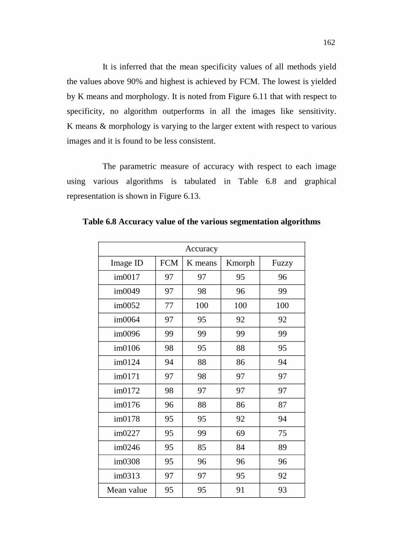
The parametric measure of accuracy with respect to each image
using various algorithms is tabulated in Table 6.8 and graphical
representation is shown in Figure 6.13.
Table 6.8 Accuracy value of the various segmentation algorithms
Accuracy
Image ID FCM K means Kmorph Fuzzy
im0017 97 97 95 96
im0049 97 98 96 99
im0052 77 100 100 100
im0064 97 95 92 92
im0096 99 99 99 99
im0106 98 95 88 95
im0124 94 88 86 94
im0171 97 98 97 97
im0172 98 97 97 97
im0176 96 88 86 87
im0178 95 95 92 94
im0227 95 99 69 75
im0246 95 85 84 89
im0308 95 96 96 96
im0313 97 97 95 92
Mean value 95 95 91 93

163
Comparision Chart - Accuracy
0
20
40
60
80
100
120
1 2 3 4 5 6 7 8 9 10 11 12 13 14 15
Images fromSTARE database
FCM Kmeans Kmorph Fuzzy
Figure 6.13 Comparison chart for the accuracy values
In the case of accuracy, FCM and K means algorithms yielded the
highest values of 95% and the other two algorithms have also yielded the
nearer values without deviating much. Like specificity, in accuracy also not a
single algorithm outperforms in all the selected images as Figure 6.13 shows.
The processing time is compared for all the algorithms and the
results are tabulated in Table 6.9 and plotted graphically in Figure 6.14.
Table 6.9 Processing time of the various segmentation algorithms
Time
Image ID FCM Kmeans Kmorph Fuzzy
im0017 03.64 1.77 2.77 13.64
im0049 06.60 1.78 3.30 09.22
im0052 09.70 2.82 2.85 21.68
im0064 06.97 3.33 3.04 17.87
im0096 10.59 3.85 2.81 15.27
im0106 11.55 3.02 2.59 17.89

164
Table 6.9 (Continued)
im0124 10.16 3.07 2.83 14.62
im0171 11.82 3.07 2.91 19.34
im0172 12.19 3.00 3.33 15.28
im0176 08.77 3.04 3.88 25.95
im0178 10.77 3.16 2.77 15.95
im0227 11.64 3.09 2.64 14.52
im0246 06.23 3.07 2.60 14.80
im0308 12.69 3.12 2.91 14.72
im0313 09.17 2.60 3.12 17.41
Mean value 09.50 2.92 2.96 17
Comparision Chart - Processing Time
0
5
10
15
20
25
30
1 2 3 4 5 6 7 8 9 10 11 12 13 14 15
Images from STARE database
FCM Kmeans Kmorph Fuzzy
Figure 6.14 Comparison chart for the processing time
It is inferred from the table and graph that the processing time for
the fuzzy is higher than the other three methods. Both the K means and
K means & morphology have lowest processing time.

165
The mean values of the results of all the tested images with regard
to different algorithms are presented in Table 6.10
Table 6.10 Mean values of results of different algorithms
Sl.No. Algorithms Mean values
SE SPE ACC Time in sec.
1 FCM 73 97 95 09.50
2 K means 88 95 95 02.92
3 K & morph 96 91 91 02.96
4 Fuzzy 91 94 93 17.00
The above table indicates that the SPE and ACC have increased in
fuzzy technique in comparison with K mean & morphological operations.
However, these values are less with respect to FCM method and it claims the
advantage of increase in sensitivity with marginal loss of SPE and ACC.
6.7 SUMMARY
The segmentation of exudates has been performed using four
different clustering algorithms like Fuzzy C means, K means, K means and
morphology and fuzzy. All the algorithms are briefed and tested on images of
STARE database and the results are presented. The algorithms are subjected
to parametric measures and the output of the different algorithms is discussed
with the aid of tables and charts. The comparative study of all the algorithms
has been presented and discussed. Suggestion has been made on the better
algorithm in segmentation process of exudates with the evidence of mean
sensitivity, specificity and accuracy. The time consumption by the various
algorithms is also presented which could be a point of research for future
researchers to expand on.


![Biomedical Research 2016; Special Issue: S414-S418 An ... · Soft exudates detection A cotton wool spot [12] is sometimes known as soft exudates. They are flat-reddish white in color](https://img.pdfslide.us/doc/110x75/5f8808f40b3bdc493932f1d0/biomedical-research-2016-special-issue-s414-s418-an-soft-exudates-detection.jpg)