Chapter 6 - Sage Publications

183

chap t e r 6

BEYOND DESCRIPTIVES

Making Inferences Based on Your Sample

Suppose you and a friend are discussing the ubiquitous use of cell phones today. You have read research suggesting that people regularly make and receive calls on their cell phones while they drive, but your friend thinks that the reports of drivers using

cell phones are exaggerated because he has not observed many people driving while talking on phones. Because you are thinking like a researcher, you are skeptical that your friend’s personal experience is sufficient evidence. Instead, you decide to examine the question scientifically.

After obtaining permission from school, you and your friend sit at an exit from a large parking deck at school and ask people leaving the deck to complete a brief survey if they were the driver of a car that just parked in the deck. The survey asks how many times drivers used their cell phone to answer or to make a call while driving to campus that day. You collect data from 10 a.m. to 3 p.m. on a Tuesday.

You find that the mean number of calls for your sample is 2.20 (SD = 0.75). These statis-tics tell you about the cell phone use of your sample of drivers—the people who drove to the school on a particular day and parked in a particular deck within a particular time. In terms of the discussion between you and your friend, however, you want to know about the cell phone use of a larger group (or population) than just those you are able to survey. In this case, you might consider the population from which your sample was drawn as all people who drive to your campus.

Recall from Chapter 4 that in order to be totally confident that you know about the cell phone use of all people who drive to your campus, you would need to survey all of them. Imagine the difficulties of trying to survey the large number of people who drive to a campus at different times and days and park at various locations. Even if you restrict your population

©SAGE Publications

184–•–RESEARCH METHODS, STATISTICS, AND APPLICATIONS

to those who come to campus and park on Tuesdays in the deck you selected, there may be some drivers who leave the parking deck by a different exit or who come to campus earlier or later than the survey period or who for some reason do not drive to campus the day you collect data. For multiple reasons, it is very unusual for a researcher to be able to collect data from every member of a population.

You might also recall from Chapter 4 that instead of finding every member of the popu-lation, researchers take a sample that is meant to be representative of the population. Probability (or random) sampling can improve the representativeness of the sample, but it is work-intensive and even with probability sampling there is no 100% guarantee of the repre-sentativeness of the sample. And how would you know if your sample is in fact representative of the population?

As an alternative method to learn about your population, you consider obtaining multiple samples of drivers to your campus in order to make sure that you have information from people who park at different lots or come at different times or days. By gathering different samples of drivers to your school, you would then be able to compare whether your first sample was representative of cell phone use among your other samples of drivers. It would take a lot of effort and time to gather multiple samples, and you still would not have data from the entire population of drivers to your campus.

As a new researcher, you might now find yourself frustrated with your options. But what if you had a statistical technique that you could use to test how well your sample represents the campus population? You could also use this statistical technique to examine how your sample’s cell phone habits compare with the research you read, or to consider if a driver’s age or gender is an important factor in their cell phone habits.

IN THIS CHAPTER, YOU WILL LEARN

• About the use of inferential statistics to determine whether the finding of a study is unusual

• The importance of the sampling distribution

• How to carry out the hypothesis testing process

• When to reject or retain a null hypothesis and the types of errors associated with each of these decisions

• The distinction between statistical significance, effect size, and practical significance

• How to compute, interpret, and report a one-sample t test comparing a sample to a known population value

zz INFERENTIAL STATISTICS

In research we often want to go beyond simply describing our sample using measures of central tendency and variability. Instead, we want to make inferences about the qualities or characteristics of the population that our sample represents. The statistics we use in this

©SAGE Publications

Chapter 6 Beyond Descriptives–•–185

process are called inferential statistics. When we use inferential statistics we draw con-clusions about a population based on the findings from a single study with a sample from the population. We do not have to repeatedly conduct the same study with different sam-ples in order to learn about the same population. Of course, replication is not a bad idea but we want to build information about populations, and inferential statistics allows us to accomplish this goal more quickly than conducting the identical study multiple times with samples from the same population.

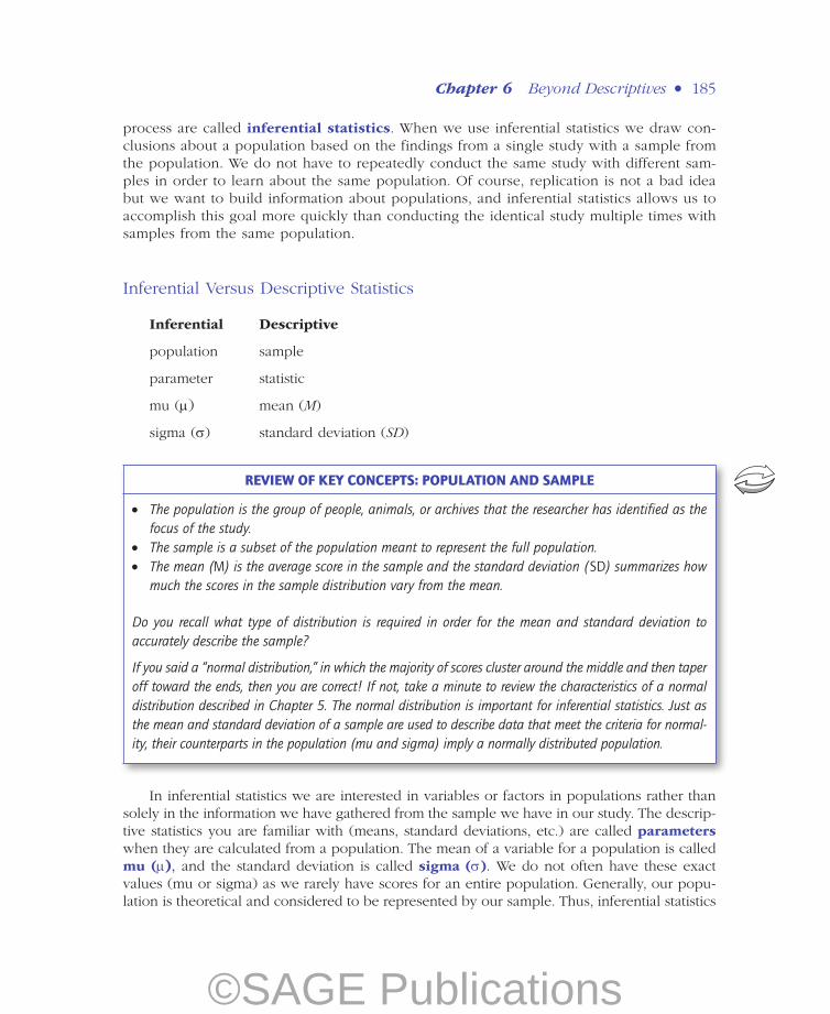
Inferential Versus Descriptive Statistics

Inferential Descriptive

population sample

parameter statistic

mu (µ) mean (M)

sigma (σ) standard deviation (SD)

REVIEW OF KEY CONCEPTS: POPULATION AND SAMPLE

• The population is the group of people, animals, or archives that the researcher has identified as the focus of the study.

• The sample is a subset of the population meant to represent the full population. • The mean (M) is the average score in the sample and the standard deviation (SD) summarizes how

much the scores in the sample distribution vary from the mean.

Do you recall what type of distribution is required in order for the mean and standard deviation to accurately describe the sample?

If you said a “normal distribution,” in which the majority of scores cluster around the middle and then taper off toward the ends, then you are correct! If not, take a minute to review the characteristics of a normal distribution described in Chapter 5. The normal distribution is important for inferential statistics. Just as the mean and standard deviation of a sample are used to describe data that meet the criteria for normal-ity, their counterparts in the population (mu and sigma) imply a normally distributed population.

In inferential statistics we are interested in variables or factors in populations rather than solely in the information we have gathered from the sample we have in our study. The descrip-tive statistics you are familiar with (means, standard deviations, etc.) are called parameters when they are calculated from a population. The mean of a variable for a population is called mu (µ), and the standard deviation is called sigma (σ). We do not often have these exact values (mu or sigma) as we rarely have scores for an entire population. Generally, our popu-lation is theoretical and considered to be represented by our sample. Thus, inferential statistics

©SAGE Publications


use descriptive statistics from our sample to make assumptions about a particular population from which our sample is drawn. When we use inferential statistics, we ask the question: Is our sample representative of our population? In other words, does our sample seem to belong to the population or is it different enough that it likely represents a totally different population?

Inferential statistics: Statistical analysis of data gathered from a sample to draw conclusions about a population from which the sample is drawn.

Parameters: Statistics from a population.

Mu (µ): Population mean.

Sigma (σ): Population standard deviation.

So the previous paragraphs do not sound like gobbledygook, let’s look at a specific example:When given the opportunity to do so anonymously, do students at University Anxious

(UA) report plagiarism more or less than the national statistics for this measure? This question involves both a sample (students at UA) and a population (national statistics for reports of plagiarism by college students). Suppose the national average for reporting plagiarism is 1%, while the UA students’ reporting average is 3%. Would you believe that UA students report plagiarism more frequently than the national average? What if the UA reporting average is 10%?; 15%? At what point do you consider the UA average to be different enough from the national average to pay attention to or to believe that the UA students are somehow different from the national population of college students?

What we are asking is, when does a difference in scores make a difference? In other words, when is a difference significant?

Probability Theory

Inferential statistics are based on probability theory, which examines random events such as the roll of dice or toss of a coin. When random events are repeated, they then establish a pattern. For example, we could toss a coin multiple times to see the number of heads and tails that result. We would expect to get heads approximately 50% of the time and tails approx-imately 50% of the time, especially if we toss the coin a large number of times. In probability theory each individual random event (in our example the outcome of one coin toss) is

assumed to be independent, which means that the outcome of each coin toss is not affected by the out-come of previous tosses. Another way to say this is that each time we toss a coin, the outcome of our toss is not affected by whether we got a head or a tail on the last or earlier coin tosses. The pattern that results from repeating a set of random events a large number of

“There is a very easy way to return from a casino with a small fortune: go there with a large one.”

—Jack Yelton

©SAGE Publications


times is used in statistics to determine whether a particular set or sample of random events (e.g., 8 heads in 10 coin tosses) is typical or unusual.

Going back to our students at UA and their reporting rate for plagiarism, we use infer-ential statistics (based on probability theory) to answer the question: Is there a significant difference between the scores at UA and the national average? We want to know if an event (the average percentage of UA students reporting plagiarism) is common or is unusual relative to the population (the national average in reporting plagiarism). We use the results from inferential statistics to make judgments about the meaning of our study. As the quote above about gambling implies, it is important to understand the probability of events occurring—many people who gamble assume that “hitting the jackpot” is a common out-come of gambling, while in reality winning large sums of money is a very rare occurrence. Of course, the success of casinos and lottery systems depends on people believing that they will be that one lucky person in a million or even one in 10 million.

In research, we pay attention to the likelihood of scores or findings occurring and we use probability theory to help us determine whether a finding is unusual. An easy way to under-stand how probability theory aids our decision making is to think about the coin toss. If we flip a coin 100 times and we get 45 heads and 55 tails, we usually do not take note of the event. If, however, we flip the coin 100 times and get 10 heads and 90 tails, we begin to won-der if our coin is weighted or different in some way. We expect to get close to the same number of heads and tails (in this case, 50 heads and 50 tails out of 100 tosses) and assume that results that differ a great deal from this expectation may indicate something unusual about the coin. But how different from our expectation do our results need to be for us to believe that there is something unusual about the coin? We may begin to be suspicious if we get 20 heads and 80 tails but that result could occur even with a “regular” coin.

Probability theory allows us to determine how likely it is that our coin toss results would have occurred in our particular circumstances. In other words, what is the probability that we would get 45 heads and 55 tails if we tossed a coin 100 times? The probability of our results is based on a theoretical distribution where a task (flipping the coin 100 times) is repeated an infinite number of times and the distribution shows how frequently any combination (of heads and tails) occurs in a certain number of repetitions (100 flips of a coin). We find out that we are likely to get 45 or fewer heads 18.4% of the time when a coin is tossed 100 times. (Of course, the same coin would need to be tossed in the same way each time in order for our results to be reliable.)

But if we tossed our coin and got 10 heads and 90 tails, we would learn that we are likely to get 10 or fewer heads only .0000000001% of the time. We then are suspicious that our coin is not typical. We cannot say whether our coin was deliberately weighted or was malformed when it was minted, only that it has a very low probability of being a normal coin. We have to recognize that although 10 heads and 90 tails is a highly unusual result from 100 coin tosses, it is possible to get this result on very, very rare occasions with a normal coin. Thus, while we may decide that our results (10 heads/90 tails) are too unusual for our coin to be normal, we also have to recognize that we may be mistaken and may have obtained very rare results with a normal coin.

All this is to say that researchers make decisions based on the probability of a finding occurring within certain circumstances. So how rare or unusual does a finding have to be in order for us to believe that the finding is significantly different from the comparison distribution

©SAGE Publications


(in this case, a distribution produced by tossing a coin 100 times an infinite number of times)? In statistics, we have adopted a standard such that we are willing to say that our result does not belong to a distribution if we find that our result would be likely to occur less than 5% of the time. So if we get a combination of heads and tails that would occur less than 5% of the time with a normal coin, we are willing to say that our coin is significantly different from a normal coin. Our research questions are much more complex than a coin toss, but they are based on examining when a difference is significant. In statistics, we call this process of decision making hypothesis testing.

Hypothesis testing: The process of determining the probability of obtaining a particular result or set of results.

Sampling distribution: A distribution of some statistic obtained from multiple samples of the same size drawn from the same population (e.g., a distribution of means from many samples of 30 students).

Sampling Distribution Versus Frequency Distribution

In order to decide whether an outcome is unusual, we compare it to a theoretical sampling distribution. In Chapter 5, we used the term frequency of scores to describe distributions composed of individual scores. In contrast, a sampling distribution is composed of a large number of a specific statistic, such as a mean (M), gathered from samples similar to the one in our study.

Let’s go back to our previous example where we flipped a coin 100 times and recorded the number of heads and tails. The sampling distribution we compare our results to is composed of scores (# of heads and # of tails) from tossing a coin 100 times and then repeating this exercise an infinite number of times. Each “score” on the distribution represents the findings from tossing a coin 100 times. The coin is tossed many hundreds of times and a distribution is then built from all these results. Thus, we have a large number of scores from samples of 100 tosses, which give the distribution the name sampling distribution. Of course, no one actually tosses a coin thou-sands of times—statisticians build the distribution based on probability.

So far we have been talking about comparing a sample to a population. Many times, however, researchers are interested in comparing two populations. For example, we might want to know if students who major in business text more than students who major in psy-chology. In this case, our sampling distribution would be created in a multistep process. First, we would ask a sample of business students and a sample of psychology students how fre-quently they text (say, in a 24-hour period). We would then calculate the mean texting fre-quency for each sample and subtract one mean from another. We would repeat this process a large number of times and create a distribution of mean differences, which would serve as our sampling distribution. If the difference in texting frequency between the population of psychology students and the population of business students is 5, then we would expect that most of the mean differences we found for our two samples would be close to 5. As we moved farther above or below 5 (as the mean difference), we would expect fewer of our pairs of samples to show these differences.

©SAGE Publications


To sum up this section: Inferential statistics allow us to determine whether the outcome of our study is typical or unusual in comparison to our sampling distribution.

Example of Hypothesis Testing

Ziefle and Bay (2005) investigated the effect of age and phone complexity on several variables related to phone use. Participants were divided into an older group (50–65) and a younger group (20–30). Phone complexity was operationally defined as the number of steps required by each phone to accomplish each of four tasks (calling a number from the phone directory, sending a text message, time to edit a number in the directory, and hiding one’s phone number from the receiver of a call).

The Siemens phone had been determined by the researchers to be more complex than the Nokia phone. Participants completed each of the four tasks using either the Siemens or Nokia phone. Although there was no difference in the number of tasks completed with each phone, participants using the more complex Siemens phone took significantly longer to complete the tasks (M = 4 min 16 sec, SD = 111 sec) than those using the Nokia phone (M = 2 min 37 sec, SD = 86 sec). Those using the Siemens phone also made significantly more “detours” (missteps) in solving the tasks (M = 130.80; SD = 62; Nokia M = 61.60; SD = 43).

Why can we say that the means for task-solving time and missteps are significantly different for the two phones as a function of the complexity of the phone? How can we determine that the differences are not just random or due to chance?

Hypothesis testing is a process that includes the use of inferential statistics and allows us to determine when the differences in time and detours are not likely to be due to chance alone.

APPLICATION 6.1

HYPOTHESIS TESTING z

Now that you understand a bit about probability theory and sampling distributions, we will incorporate this knowledge into the process we use to examine research findings. This process is called hypothesis testing and uses statistics to analyze the data. As a researcher, you should always plan your statistical analysis before you conduct your study. If you do not consider how to analyze your data as you design your study, you might collect data that cannot be analyzed or that will not adequately test your hypothesis.

Null and Alternative Hypotheses

After identifying your variable(s) for your study, you should state what you expect to find or your prediction for your study, which is called the alternative hypothesis (Ha). In experimental

©SAGE Publications


research this prediction is called the experimental hypothesis (Ha) and is always stated in terms of predicting differences between groups. Alternative and experimental hypotheses are both predictions but they are not the same because all experimental hypotheses are also alterna-tive hypotheses, but many alternative hypotheses are not experimental.

In the simplest case for an experiment, we compare our sample to some population value. Your experimental hypothesis will predict a difference between your sample and the popula-tion on the variable that you measure. For example, we may hypothesize that psychology majors are more likely to text than college students in general. In this case, we would compare the mean texting frequency for a sample of psychology majors and the mean texting fre-quency for the population of college students.

We contrast the experimental hypothesis with the null hypothesis (H0), which is stated in terms of no difference. The null hypothesis is important to state because that’s actually what we test in a study. It sets up the sampling distribution that we will compare our results to. In terms of the example above, the null hypothesis would predict that you would find no differ-ence in texting frequency between your sample of psychology majors and the texting fre-quency of the population of college students.

Alternative hypothesis (Ha): A prediction of what the researcher expects to find in a study.

Experimental hypothesis (Ha): An alternative hypothesis for an experiment stated in terms of differ-ences between groups.

Null hypothesis (H0): A prediction of no difference between groups; the hypothesis the researcher expects to reject.

A study should always be designed to find a difference between treatments, groups, and so on, and thus to reject the null hypothesis. Many novice researchers (usually students just learning about research) will mistakenly design a study to support their null hypothesis, which means that they will try to show that there is no difference between their sample and the population. Such studies will not further our knowledge, because we do not learn anything new about the variable(s) of interest.

Rejecting the Null Hypothesis

After designing a study and collecting data, we need to make a decision about whether we can reject our null hypothesis, H0, and support our alternative hypothesis, Ha. In order to decide, we select a statistical test to compare our results (for the variable we have measured) to a theoretical sampling distribution. Remember that our sampling distribution is defined by the null hypothesis. In our study examining the texting behavior of psychology majors, our sampling distribution is created by collecting information about the texting frequency of hundreds of samples of college students and computing a mean texting frequency for each

©SAGE Publications


sample. We then have a distribution that is composed of the hundreds of texting frequency means—remember the “scores” in a sampling distribution are always a statistic—in this case our “scores” are the means of texting frequency for each sample of college students.

PRACTICE 6.1

NULL AND ALTERNATIVE HYPOTHESES

Go back to Application 6.1 earlier in this chapter and review the study by Ziefle and Bay (2005).

1. State null and alternative hypotheses for the impact of phone complexity on the time it takes to complete a series of tasks using the phone. Remember, the Siemens phone had been deter-mined to be more complex than the Nokia phone.

2. Now develop null and alternative hypotheses that might make sense to examine the impact of age on the use of cell phones. Remember that the study used two age groups: older (50–65) and younger (20–30). You do not have information about what the researchers found in terms of age but what might you predict they would find?

See Appendix A to check your answers.

REVIEW OF KEY CONCEPTS: THE NORMAL DISTRIBUTION

1. What are the characteristics of a normal distribution?

2. What characteristics of a normal distribution allow us to make assumptions about where scores fall or statistics fall in the case of a sampling distribution?

You know your normal distribution facts if you answered bell shaped and symmetrical; the mean, median and mode are identical; and the range is defined by the mean plus or minus 3 standard deviations. Most scores cluster around the mean, and the frequency of scores decrease as they are increasingly higher or lower than the mean.

The area under the curve of a normal distribution is distributed so that 50% of the distribution lies on either side of the mean; approximately 68% of the distribution lies between the mean and plus and minus 1 SD, 95% of the distribution lies between the mean and plus and minus 2 SDs, and 99% of the distribution lies between the mean and plus and minus 3 SDs. As we learned in Chapter 5, we can even determine the exact percentile of any score and thus where it falls in a normal distribution using z scores and the z table.

©SAGE Publications


The sampling distribution shows the values that would occur if our null hypothesis is true—in our example this would occur if the texting frequency of psychology students did not differ from that of all college students. Sampling distributions are normally distributed and have the same characteristics as normally distributed frequency distributions—they are sym-metrical and the range is defined by the mean plus or minus 3 standard deviations (M ±3 SD). Most scores fall around the mean—you learned in Chapter 5 that the majority of the distribu-tion (approximately 68%) falls within plus or minus 1 standard deviation from the mean. Approximately 95% of a normal distribution is found within 2 standard deviations above and 2 standard deviations below the mean, and approximately 99% of the distribution falls between ±3 standard deviations from the mean.

Because the normal distribution is symmetrical, the percentage of the distribution on each side of the mean is identical. For example, you know that approximately 95% of a normal distribution is found within ±2 standard deviations from the mean. That means that 47.5% of the distribution is between the mean and the value representing 2 standard deviations above the mean, and 47.5% of the distribution is found between the mean and the value represent-ing 2 standard deviations below the mean. In addition, we know what percentage of the distribution lies outside of ±2 standard deviations. If 95% of the distribution is between ±2 standard deviations, then 5% lies outside this range. Because the distribution is symmetrical, the remaining 5% is split between the top and the bottom of the distribution. So, 2.5% of the distribution falls above the value that represents the mean plus 2 standard deviations, and 2.5% of the distribution falls below the mean minus 2 standard deviations. Figure 6.1 shows a nor-mal distribution and the percentage of the distribution that is found within the range of values represented by 1, 2, and 3 standard deviations from the mean.

Figure 6.1 Theoretical Normal Distribution With Percentage of Values From the Mean to

1, 2, and 3 Standard Deviations (Sigma)

±1 SD

−3 σ −2 σ −1 σ µ +1 σ +2 σ +3 σ

±3 SD

±2 SD

0.1%0.1%2.1% 2.1%

13.6%13.6%

34.1%34.1%

©SAGE Publications


In the coin toss example discussed earlier in the chapter, we tossed a coin 100 times and got 45 heads and 55 tails. We can compare these results to a sampling distribution. In the case of the coin toss, we would predict that we would have 50% heads and 50% tails, so for 100 tosses we would predict 50 heads and 50 tails. Our sampling distribution would show most instances of 100 tosses would result in close to the 50:50 split of heads and tails, and our result of 45 heads would not be unusual. As results are more and more different from the 50:50 split, however, the frequency of such results would decrease until you find that very few 100 tosses resulted in 90 heads and 10 tails and even fewer tosses resulted in 99 heads and 1 tail. This latter finding (99 heads and 1 tail) would be found in the far tail of the sampling distribution because it would occur very rarely out of 100 tosses.

Let’s also consider the texting frequency example with specific values. Suppose the mean texting frequency of college students is 50 times per day and the standard deviation is 10. If we find for our sample of psychology students that their texting mean is 70 times per day, would we consider them to be typical of the population of college students? A mean of 70 would be 2 standard deviations above the mean of 50 and so would belong outside the mid-dle 95% of the distribution. If, however, the psychology students’ mean was 45, this sample mean would be .5 standard deviations below the population mean and is within the middle 68% of the distribution. We would consider the first mean (70) to be rare for the population of all college students, while the second mean (45) occurs frequently within a population distribution with a mean of 50.

A normal distribution (such as a sampling distribution) is a theoretical distribution, and its characteristics can be applied to any M and SD. Thus, the characteristics of the distribution remain the same whether the M = 55, SD = 5 or the M = 150, SD = 25. Test your understand-ing of the information you have just learned. If the M = 55, what range of scores would define 68% of the distribution? Stop reading now and see if you can figure this out.

Answer: If you added 5 to 55 and subtracted 5 from 55 to get 50–60 as the range, you are correct. You have learned that 68% of a normal distribution is defined by the mean plus and minus 1 standard deviation. In this case, 50 equals the mean minus 1 standard deviation (55 − 5) and 60 equals the mean plus 1 standard deviation (55 + 5). Now that you know this, calculate the range of scores that defines 68% of the distribution when the M = 150, SD = 25. Check with your classmates or teacher if you are unsure that you have done this correctly. Now calculate the range of scores representing the middle 95% of the distribution when M = 55, SD = 5. You should get 45–65. You multiply the SD by 2 and then add and subtract that value to the M [55 ± (2 × 5)] or 55 ± 10 = 45–65.

If a distribution is normal, given any M, SD combination, we can figure out the range of scores expected for that distribution and the percentage of scores lying within specific values. We can then figure out whether we believe that a value is likely to be found within that dis-tribution. For example, if you knew that the M = 55, SD = 5 for some test and I told you I scored a 60 on the test, would you believe that my score could have come from the M = 55, SD = 5 distribution? What if I told you I scored 90? In the first example, it is quite likely that I could belong to the M = 55, SD = 5 distribution as my score of 60 is only 1 SD above the mean. However, if I scored 90, my score would be 7 SD above the mean, and it is very unlikely that I took the test that had M = 55, SD = 5. This decision-making process reflects the process we use in hypothesis testing.

©SAGE Publications


The area of a sampling distribution that researchers/psychologists usually focus on is 95% of the distribution and the values lying outside this region. We refer to 95% of the distribution as the region of acceptance and the 5% lying outside the region of acceptance as the region of rejection. Figure 6.2 provides a pictorial representation of these areas of a distribution. These regions then determine what decision we make about the null hypothesis for our study. If the result from our statistical test is in the region of acceptance, we accept or retain our null hypothesis. This suggests that our statistical finding is likely to occur in a sampling distribution defined by our null hypothesis. (If this statement seems confusing, think of the example above where I had a score of 60 on a test and compared my score to a distribution of test scores with M = 55, SD = 5). If our finding is in the region of rejection (in the extreme 5% of the distribution), we reject the null hypothesis. In rejecting the null hypothesis, we are implying that we think that our finding would rarely occur in the sampling distribution by chance alone; in fact, it would occur only 5% or less of the time. Think of the example above where I scored 90, which was also compared to a distribution of test scores where M = 55, SD = 5.

If our decision is to reject the null hypothesis, this decision implies that we have sup-ported our alternative or experimental hypothesis. This is the goal we hope to achieve in all our studies—to reject the null and to accept the alternative/experimental hypothesis. When our findings fall in the region of rejection and we reject the null hypothesis, we state that we have found statistical significance (or a statistically significant difference) between the sample and the sampling distribution that we are comparing. If we find significance, we can conclude that our sample must have come from a different distribution than the one defined by our null hypothesis.

Figure 6.2 Regions of Rejection and Regions of Acceptance for a Two-Tailed Test at p < .05

Region ofAcceptance

Region ofRejection

Region ofRejection

Highest2.5%

Lowest2.5%

µ

©SAGE Publications


Region of acceptance: Area of sampling distribution generally defined by the mean ±2 SD or 95% of the distribution; results falling in this region imply that our sample belongs to the sampling dis-tribution defined by the H0 and result in the researcher retaining the H0.

Region of rejection: The extreme 5% (generally) of a sampling distribution; results falling in this area imply that our sample does not belong to the sampling distribution defined by the H0 and result in the researcher rejecting the H0 and accepting the Ha.

Statistical significance: When the results of a study fall in the extreme 5% (or 1% if you use a more stringent criterion) of the sampling distribution, suggesting that the obtained findings are not due to chance alone and do not belong to the sampling distribution defined by the H0.

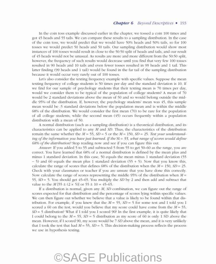
The cartoon in Figure 6.3 should help you to see (and remember) that a difference must be in the region of rejection before it is considered statistically significant.

Testing a One-Tailed Versus a Two-Tailed Hypothesis

Let’s add a few more details to the process of statistical significance testing. Don’t worry—these additional details are not difficult to understand, and we will summarize everything once we have covered all the details of hypothesis testing. When we state our hypotheses, we can

Figure 6.3 Difference Versus Statistical Difference

Why don’tyou eversmile?

I amsee. . . Nope

Whataboutnow?

Notquite Now??

Now that’s astatisticallysigni�cant

smile!!

Source: Sandi Coon

The hypothesis testing process allows us to go beyond our individual judgment of what is different and determine the probability that our results are significantly different.

©SAGE Publications


state them in one of two ways—as a one-tailed or a two-tailed hypothesis. Thus far, we have considered only two-tailed hypotheses. We have assumed that we had two regions of rejection, one at the very bottom of the distribution and one at the very top of the distribution (see Figure 6.4, graph a). In a two-tailed hypothesis, we do not care whether our computed value from our study falls in the very bottom or in the very top of our sampling distribution. So our regions of rejection are in both tails of the distribution; hence, the term two-tailed hypothesis. We sometimes refer to a two-tailed hypothesis as a nondirectional hypothesis because we are predicting that our findings will fall in either the very top or very bottom of our sampling distribution.

In a normal distribution, the extreme top or bottom 2.5% of the distribution is defined by 1.96 standard deviations from the mean. This value (±1.96 in a normal distribution) is called the critical value, and it defines the region of rejection for a two-tailed test. Results that are more than 1.96 standard deviations above or below the mean in a normal distribution fall in the extreme upper or lower 5% of the distribution (or in the region of rejection). When this happens, we can reject our null hypothesis. Different statistical tests have different critical values to define the region of rejection. You will learn about these values in later chapters.

In contrast, a one-tailed hypothesis predicts that our computed value will be found in either the very top or the very bottom of the sampling distribution. In a one-tailed hypothesis, there is only one region of rejection and hence the term one-tailed hypothesis.* Sometimes we call a one-tailed hypothesis a directional hypothesis because we are predicting the direc-tion (higher or lower) of our findings relative to the mean of our sampling distribution.

In a normal distribution, the extreme top or bottom 5% of the distribution is defined as 1.645 standard deviations from the mean. This value (1.645) is the critical value for a one-tailed test that has only one region of rejection. If our results are more than 1.645 standard deviations from the mean they then fall in the extreme upper or lower 5% of the distribution, and we can reject our one-tailed null hypothesis. Figure 6.4, graph b, depicts the region of rejection for a one-tailed hypothesis.

If we correctly predict the direction of our findings, it is easier to reject our null hypoth-esis when we use a one-tailed (or directional) hypothesis as the entire region of rejection (5% of the distribution) is in one tail of a normal distribution. If we use a two-tailed test, half of the rejection region is in each tail of the distribution and so our results must be a more extreme value (in the top or bottom 2.5% of the distribution) in order to reject the null hypoth-esis. We can see from Figure 6.4, graphs a and b, why it is easier to reject our null hypothesis with a one-tailed than a two-tailed hypothesis. With the one-tailed hypothesis, we need only get a value higher than 1.645 to reject the null, but with a two-tailed hypothesis, we would need a value higher than 1.96 to reject the null hypothesis.

*H. Kimmel (1957) argued that the use of one-tailed tests should not be based on a mere wish to use a directional hypothesis and thus have a greater chance of rejecting the null. He recommended that one-tailed tests be restricted to situations (a) where theory and previous research predict a specific direction to results and a difference in the unpre-dicted direction would be meaningless; (b) when a difference in the unpredicted direction would not affect actions any differently than a finding of no difference (as when a new product is tested and assumed to be an improvement over the old product; if results show the new product is significantly worse or no different than the old product, no action will be taken); or (c) if theories other than the one the researcher supports do not predict results in a direction different from the one-tailed hypothesis.

©SAGE Publications


Two-tailed hypothesis: A hypothesis stating that results from a sample will differ from the population or another group but without stating how the results will differ.

One-tailed hypothesis: A hypothesis stating the direction (higher or lower) in which a sample statistic will differ from the population or another group.

Critical value: The value of a statistic that defines the extreme 5% of a distribution for a one-tailed hypothesis or the extreme 2.5% of the distribution for a two-tailed test.

Let’s consider an example to illustrate the one- and two-tailed areas of rejection. For a two-tailed area of rejection we are interested in any scores falling outside the middle 95% of the sampling distribution. Remember that the µ ± 2 σ defines the middle 95% of the sampling distribution. Note that we are using parameters (µ and σ) because we are considering the population rather than a sample. In terms of the example of text messaging that we used previously, we found a mean of 50 for the population of college students with a standard deviation of 10. This means that for a two-tailed hypothesis, 50 ± 2 (10) defines the cutoff values for our region of rejection. Scores below 30 and above 70 fall in the region of rejection.

When we consider a one-tailed test, the region of rejection is the top or bottom 95% of the distribution. In this case, the region of rejection is defined by half of the distribution (50%) plus 45% of the other half of the distribution. In a normal distribution, the µ + or – 1.64 σ defines

Region ofAcceptance

Region ofAcceptance

(a) Two-tailed test

-1.96 1.96 1.6450 0

(b) One-tailed test

Region ofRejection

5%

Region ofRejection

2.5%

Region ofRejection

2.5%

Note: Shaded areas represent regions of rejection for one-tailed and two-tailed tests at the .05 criterion level. Unshaded area under the curve is the region of acceptance for the tests. Critical values define the region of rejection (±1.96 for the two-tailed test and ±1.645 for the one-tailed test).

Figure 6.4 Regions of Rejection and Regions of Acceptance for One- and Two-Tailed

Tests Using a Normal Distribution

©SAGE Publications


the region of rejection depending on whether our region is above or below the mean. Again using µ = 50 and σ = 10, we have 50 + 1.64(10) or 50 − 1.64 (10) to define the cutoff value for the region of rejection for a one-tailed test. So if we think our sample of psychology majors texts more than the population of college students we would use 66.4 (50 + 16.4) as the score defining our region of rejection. If we predict that our sample will text less than the population of college students, we would use 33.6 (50 − 16.4) as the score defining our region of rejection. We can see that the two-tailed test must have a higher (70 vs. 66.4) or lower (30 vs. 33.6) value than the one-tailed test in order for the value to fall in the region of rejection.

Most of the time we use a two-tailed or nondirectional hypothesis in hypothesis testing so that we can reject findings that are rare for our distribution, regardless of the tail in which the findings fall. In addition, as we saw above, we have a more stringent test using a two-tailed test. Thus, even when we have a directional hypothesis, most researchers still use a two-tailed test.

Setting the Criterion Level (p)

In addition to deciding about the type of hypothesis (one- or two-tailed) we wish to test, we have to decide the criterion level (p) for our region of rejection. Thus far, you have learned about the .05 criterion level, where 5% of the sampling distribution is defined as the region of rejection. As stated earlier, this criterion level is the most common level selected for hypothe-sis testing. This means that given your sampling distribution you will reject results that occur

PRACTICE 6.2

ONE-TAILED AND TWO-TAILED HYPOTHESES

1. Are the following alternative hypotheses directional or nondirectional? One- or two-tailed?

a. Ha: Students with low verbal ability are more likely to plagiarize than those with high verbal ability.

b. Ha: Psychology majors will exhibit more interpersonal skills in a new situation than students in other majors.

c. Ha: Single adults who use online dating services will differ in a measure of shyness than single adults who do not use online dating services.

d. Ha: Those who report high levels of stress will be more likely to over-eat than those who report low levels of stress.

2. Which alternative hypothesis results in a more stringent test? Explain your answer.


©SAGE Publications


less than 5% of the time by chance alone. Another way to say this is that the probability (hence the symbol p) is less than 5% that you will get these results by chance alone given your sam-pling distribution.

Suppose, however, that you want to be more confident that your findings do not belong on the sampling distribution defined by your null hypothesis. Then, you might select the more stringent .01 criterion level, where the region of rejection is composed of only 1% of the sam-pling distribution. Using the .01 criterion with a two-tailed hypothesis, the lowest .5% (or .005) and the highest .5% of the sampling distribution are defined as the region of rejection. If you use the .01 criterion with a one-tailed hypothesis, then the very bottom 1% or the very top 1% of the sampling distribution makes up the region of rejection. Obviously, it is more difficult to reject the null hypothesis using the .01 level, as the region of rejection is much smaller than when one uses the .05 level.

Criterion level: The percentage of a sampling distribution that the researcher selects for the region of rejection; typically researchers use less than 5% (p < .05).

All this is to say that you as the researcher serve as the decision maker in the hypothesis testing process. You determine the null and alternative hypotheses, type of hypothesis (one- vs. two-tailed), and criterion level (.05 vs. .01). Of course, there are some standards to follow. You can’t just say that your criterion for significance is 50%. Researchers agree that 5% is an acceptable amount of error, but this number is not set in stone. When results show a signifi-cance level between .051 and .10, researchers may describe them as “approaching signifi-cance,” particularly if there was a very small sample size or the research was a pilot study. Such results can suggest to the researchers that their hypothesis deserves further study. They may then replicate the study with tighter controls or examine their methodology for ways to better measure their variables or to implement their treatment. In any case, researchers should always be aware that the less stringent the criterion level, the more likely they have made an error in deciding to reject the null hypothesis. Researchers must also be aware of the possi-bility for error if the null hypothesis is not rejected (is retained).

• State null hypothesis—H0 • State alternative hypothesis—Ha one-tailed or two-tailed hypothesis? • Define sampling distribution and region of rejection criterion

level—.05 or .01? • Collect data and compute appropriate statistical test • Compare results to sampling distribution • Decide whether to reject or retain null hypothesis • Consider the possibility of error in your results

Table 6.1 Hypothesis Testing Process

©SAGE Publications


zz ERRORS IN HYPOTHESIS TESTING

Once you have named null and alternative hypotheses and your criterion level, you compute a statistical test and compare the finding to the sampling distribution defined by your null hypothesis. If the finding falls in the region of acceptance, you retain the null hypothesis and assume that you do not have support for the alternative hypothesis. If the finding falls in the region of rejection, however, you reject the null hypothesis and accept or support the alterna-tive hypothesis. You can assume that the findings are so different from those predicted by the null hypothesis that they are not part of the sampling distribution defined by the null hypoth-esis. Although the finding is rare for the sampling distribution (as they are found in the extreme top or bottom of the distribution), they still could occur in the sampling distribution by chance.

Note that in the statistical significance testing process we use the phrases “reject” or “retain” the null hypothesis and “support/accept” or “not support” the alternative hypothesis. We do not say that we “proved” the alternative hypothesis because we are working with prob-ability in inferential statistics. We know that even when there is a very high probability that what we find is correct, there is always a small (sometimes a minuscule) chance that we are wrong and that what we have found is in fact a very rare occurrence for a true null hypoth-esis. Or there is a chance that our finding belongs on a different distribution but because of this different distribution’s overlap with our sampling distribution, it appears that our finding belongs to the sampling distribution. Because there is always a chance for error, we never prove any of our hypotheses but instead support or do not support our hypotheses. Probability and inferential statistics allow us to feel confident that our chance of error is small, but we can never say with absolute finality that we have proven a hypothesis.

Type I and Type II Errors

Think of a class where you usually do very well on assignments and then for some reason you make a very low and unexpected grade. The low grade does not represent your typi-cal performance in the class, but it is still a grade that will be included in your range of scores for the class. When we reject the null hypothesis, we must understand that our finding could have occurred (just like the low grade), although rarely, within the distribu-tion of scores for our sampling distribution. Thus, there is always the chance that we are making an erroneous decision by rejecting the null hypothesis—this error is called a Type I error and is formally defined as incorrectly rejecting a true null hypothesis. The proba-bility of making a Type I error is determined by the criterion level you have used in your hypothesis testing. If you reject the null hypothesis using the .05 criterion level, then the findings are in the extreme 5% of the distribution and the probability of a Type I error is 5%. Similarly, if you reject the null hypothesis using the .01 level, then the probability of making a Type I error is 1%.

If you retain the null hypothesis there is also a probability of making an error. In this case, although the results fall within the expected middle range of values in the sampling

©SAGE Publications


distribution (region of acceptance), they could still belong to a different distribution whose scores overlap with the sampling distribution defined by the H0. This type of error (incor-rectly retaining the null hypothesis) is called a Type II error. In this book, we will not calculate the probability of such an error; it is sufficient that you know when a Type II error may have occurred (hint: whenever you retain the null hypothesis). In hypothesis testing, because you are basing your decision on the probability of a result belonging to a distribu-tion by chance, regardless of the decision you make there is some probability that you have made an error.

Type I error: The probability of rejecting a true H0 ; defined by the probability of the significance level of your findings.

Type II error: The probability of incorrectly retaining a false H0 .

In summary, whenever you reject the null hypothesis, there is a probability that you have made a Type I error, and the probability of this error is equal to the p value that you use to reject the null hypothesis. If you reject the null hypothesis at the p < .05 level, there is less than a 5% probability that you have made a Type I error. On the other hand, if you retain the null hypothesis, there is the probability that you have made a Type II error. Without additional (and quite complex) calculations, you do not know the exact probability of a Type II error but should be aware of the possibility. Because you cannot both reject and retain the null hypothesis at the same time, there is a probability of either a Type I or a Type II error based on your decision to reject or retain the null. Therefore, if you reject the null hypothe-sis there is the probability of a Type I error but 0% chance of a Type II error. If you retain the null hypothesis there is a probability of a Type II error but 0% chance of a Type I error.

Table 6.2 illustrates the four possible outcomes of hypothesis testing that we have explained above. The null hypothesis can be either true or false and you can either retain or

Table 6.2 Four Possible Outcomes in Statistical Significance Testing

Decision Based on Observed Results

Reject Retain

Reality (not directly observed or tested)

H0 is True Type I errorA

CorrectB

H0 is False CorrectC

Type II errorD

©SAGE Publications


reject it. If the null hypothesis is true and you reject it, you have made a Type I error (cell A). Another way to say this is your findings appear to belong in the region of rejection but actually are a value that by chance rarely occurs in the distribution. Figure 6.5 provides an example of a Type I error that may help you distinguish this error. Alternatively, if the null hypothe-sis is true and you retain it then you have made a correct decision (cell B). If the null hypothesis is false and you reject it, you have made a correct deci-sion (cell C). If the null hypothesis is false and you fail to reject it, you have made a Type II error (cell D).

In designing and carrying out a study, you make every effort to cor-rectly reject a false null hypothesis (cell C), which is called power, and to avoid making an error in your decision

making (cells A and D). There are multiple steps you can take to increase the power of your study, which are described under the section “Reducing the Chance of a Type II Error.”

Figure 6.5 A Type I Error

I don’t get it. . .The study saideating 4oz of

chocolate a daymakes you LOSE

weight!!?

A humorous example of a potential Type I error you want to avoid . . . assuming (or finding) a difference when there isn’t really one.

Applying the Complete Hypothesis Testing Process in a Study

Let’s now apply the hypothesis testing process to the Ziefle and Bay (2005) study that was briefly described at the beginning of the chapter. We will limit our focus right now to their investigation of the effect of phone complexity on time to complete four tasks (calling a number from the phone directory, sending a text message, editing a number in the directory, and hiding one’s phone number from the receiver of a call). Remember that the researchers had determined that the Siemens phone was more complex than the Nokia phone.

A possible null hypothesis would be that there is no difference in the time it takes to complete the tasks using the Siemens or the Nokia phone. A nondirectional (two-tailed) alternative hypothesis

APPLICATION 6.2

©SAGE Publications


would state that the phones would require different times to complete the tasks, while a directional (one-tailed) hypothesis would state that the Siemens phone would take more time to complete the tasks than the Nokia phone. Either one of these hypotheses is acceptable, but they have different implications for the region of rejection.

If we select a .05 criterion level, then for the nondirectional Ha we will reject the H0 if the results fall either at the bottom 2.5% or top 2.5% of the distribution defined by the null hypothesis. If we state a directional H0 then we will reject the H0 only if our results fall in the direction that we pre-dicted (that those using the Siemens phone took more time to complete a task than those using the Nokia phone). If we find that those using the Nokia phone took more time to complete the task, we cannot reject our directional H0 because our results are in the wrong direction from our region of rejection.

Remember that most of the time we use a two-tailed or nondirectional hypothesis in hypothesis testing so that we can reject findings that are rare for our distribution, regardless of the tail in which the findings fall. In addition, a two-tailed hypothesis is a more stringent test than using a directional hypothesis because even when we have correctly predicted the direction of our findings (that the Siemens phone will require more time to complete a task than the Nokia phone), given a certain criterion level (say .05), our region of rejection in each tail of the distribution is half (2.5%) of what it would be for a one-tailed test (5%) in the predicted tail of the distribution.

The results of the statistical test used by Ziefle and Bay (2005) fell in the region of rejection (top or bottom 2.5% of the distribution) and allowed them to conclude that they had found statistical significance. They could then reject the null hypothesis and support the alternative hypothesis that the Siemens phone takes longer to complete four tasks than the Nokia phone. Another way to state the results is to say that the results show that the Siemens phone takes significantly longer to com-plete four tasks than the Nokia phone. We understand that with this decision, there is a 5% chance of having made a Type I error. If, on the other hand, their results had fallen in the region of accep-tance, they would have decided to retain the H0 and concluded that there is no difference in the amount of time it takes to complete tasks using the Siemens or the Nokia phone. In this case, there would have been a probability of a Type II error but we do not know its exact probability.

Reducing the Chance of a Type I Error

When you reject the null hypothesis the probability of a Type I error is determined by the criterion level, and you can therefore make your study less vulnerable to a Type I error by changing your criterion level. Most of the time social scientists use the p < .05 criterion as they believe that less than 5% probability of making an error is an acceptable risk.

If they are very concerned about the Type I error, they would use a more stringent crite-rion (such as p < .01). The implications of the findings of a study may lead researchers to use

©SAGE Publications


a more stringent level. If, for example, you are studying an educational program to prevent plagiarism that is inexpensive and easy to implement, you may feel very comfortable using the .05 criterion. If you inadvertently make a Type I error (incorrectly reject a true null hypoth-esis), you have not created too much of an expense or bother for those implementing the program and have not harmed the students participating in the program. If, however, your new technique is expensive in terms of dollars and teachers’ time, and intrusive in terms of students’ confidentiality, you may want to reduce the probability of a Type I error and employ the .01 criterion level.

Another common strategy to reduce Type I error is to use a two-tailed rather than a one-tailed test. Recall that the two-tailed test is a more stringent test because the regions of rejec-tion are split between the two tails of the distribution, and therefore the critical value must be more extreme in order for the results to be considered statistically significant. Although in theory a two-tailed test is used for nondirectional hypotheses, in practice most researchers use two-tailed tests for both directional and nondirectional hypotheses in order to reduce the chance of a Type I error.

PRACTICE 6.3

UNDERSTANDING THE HYPOTHESIS TESTING PROCESS

Can you enter information from the Ziefle and Bay (2005) study from Application 6.2 in the different boxes of the flow chart below?


Support Ha

Probability ofType I error

Not support Ha

Probability ofType II error

Collect data, computeappropriate statistical test, and

compare to samplingdistribution

Criterion Level.05 or .01?

One- or Two-Tailed Test?

De neSamplingDistribution

State HaState H0

RetainHa

Decision?RejectH0

©SAGE Publications


Reducing the Chance of a Type II Error

You can avoid a Type II error by choosing a less stringent criterion (such as p < .06 or p < .10), but then you run the risk of a Type I error. Fortunately, you do not need to play this back-and-forth game because there are better ways to minimize your risk of a Type II error. Consequently, set the criterion level to address Type I error and design a powerful study to address Type II error. Power is the ability to detect a statistically significant result when in fact the result exists in the population. In other words, having enough power in a study allows you to avoid the Type II error of retaining the null when the null is false.

Key factors that impact the power of a study are:

1. Sample size (larger sample size = more power)

2. Amount of error in the research design (less error = more power)

3. Strength of the effect (stronger effect = more power)

Power: The ability to reject the null hypothesis when it is, in fact, false.

Power and Sample Size

In order to have power, you must have enough members of the population represented in your sample for you to feel confident that the results you found in your study are in fact the ones that exist in the population. Thus, one way to increase power is to increase your sample size. The larger the sample size the more confident we can be that the mean of our sample approaches the mean of the pop-ulation from which the sample is drawn. Thus, we are more confident that any difference we find according to our statistical test is reliable.

Think about the example above about psychology majors’ text messaging frequency. Suppose in order to get a sample of psychology majors we ask the 10 students in a Research Methods class how many text messages they sent during the last 24 hours. How well would their data represent all psychology majors at the school if there were 260 majors?

If you answered not very well, you are correct. The class reflects students at a certain level of progress in the major, majors taking a class at a certain time with a particular teacher. The class does not include, for example, majors who are just beginning their study of psy-chology or those who have completed the Research Methods course or those who are not sure they want to continue in the major. The class may also be weighted more heavily toward one gender or ethnicity or age that is not reflective of all psychology majors. All of these factors may influence how frequently psychology majors text and thus the texting frequency of the 10 students may deviate from the texting frequency of all majors.

“It’s not about right. It’s not about wrong. It’s about power.”

–From Buffy the Vampire Slayer (2002).

©SAGE Publications


A larger sample would better reflect all the diversity of characteristics of psychology majors and provide a more reliable and less variable measure of the texting frequency of the majors. When we compare a measure derived from a large sample size to a sampling distribution, we are more likely to detect even a small difference (and significance) between the sample and our sampling distribution because of the increased stability and representativeness of the sample mean. Thus, we have increased confidence in the results of our statistical significance testing.

Power and Error in the Research Design

There are many ways to reduce error in your research study and in doing so, you increase the power of your study. The diversity of your sample can be a source of error. This is called within-groups variance (or error variance) and represents the unaccounted for differences in the sample. In our study about texting among psychology majors, texting frequency is what we are systematically studying and therefore is not considered error. However, all the other individual differences among our sample such as year in school, gender, age, and personal experiences are potential sources of error because these differences may affect the texting frequency of psychology majors. One way to reduce within-groups variance is to increase the homogeneity of the sample by limiting your population from which your sample is drawn to only senior psychology majors, or to only women, or to only those who have owned a cell phone for at least five years, and so on. Another way to reduce this type of error is to system-atically evaluate potential differences in your sample. For example, you might determine if there is a relationship between year in school and texting, or gender and texting, or if texting is related to how long someone has owned a cell phone. These strategies help you to reduce the within-groups error variance, but you can never eliminate it because some of this error is due to random (unsystematic and unpredictable) differences among individuals, or that which makes each of us unique.

Other ways to reduce error in your study are to select appropriate statistical tests (we will discuss this later in the chapter and in following chapters), reduce sampling bias (see Chapter 4), select reliable and valid measures (see Chapter 3), and choose measures that are sensitive. The sensitivity of the measurement instrument determines your ability to detect differences in quality or quantity. We have smoke detectors in our house that we hope are sensitive enough to detect the presence of smoke. Likewise, we choose measurement instruments in a research study that will be sensitive enough to detect differences in the construct we are examining. For example, at minimum we would want a measure of depression to distinguish between some-one who is depressed and someone who is not, and a more sensitive measure could further distinguish between different levels of depression (e.g., mild, moderate, extreme).

Within-groups variance (or error variance): The differences in your sample measure that are not accounted for in the study.

Homogeneity of the sample: The degree to which the members of a sample have similar characteristics.

Sensitivity: The ability of a measurement instrument to detect differences.

©SAGE Publications


Power and the Strength of the Effect

The strength of the effect refers to the magnitude or intensity of a pattern or relationship, and increases the likelihood that the pattern or relationship will be detected. The amount of smoke in your house impacts your ability to observe it, and likewise it is easier to identify strong patterns or relationships in social science constructs. For example, it is easier to detect some-one’s mood if that person is extremely happy, sad, or angry than if he or she is experiencing more mild or nuanced emotions.

The strength of the effect is something that we measure in research, and as such you do not have as much ability to directly impact it as you do with sample size and error. The extent to which you can increase the strength of the effect depends on the goal of the study and the research design. One strategy is to focus your study on phenomena known through previous research to have a strong pattern or relationship. Another strategy is to conduct an experiment that includes a strong manipulation that you hope will lead to a strong effect.

PRACTICE 6.4

INTERPRETING RESULTS

1. Which of the following results would be considered statistically significant at the p < .01 level? Select all that would be statistically significant.

(a) p = .05 (b) p = .005 (c) p = .10 (d) p = .001 (e) p = .02 (f) p = .009

2. A researcher sets the criterion level at p < .05.

(a) If the results revealed p = .10:

i. Are the results statistically significant?

ii. Would you reject or retain the null hypothesis?

iii. What type of error might you be making? Name at least two strategies to reduce this error in future research.

(b) If the results revealed p = .03:

i. Are the results statistically significant?

ii. Would you reject or retain the null hypothesis?

iii. What type of error might you be making? How might you eliminate this error, and what would the consequences of that be?

(Continued)

©SAGE Publications


zz EFFECT SIZE AND PRACTICAL SIGNIFICANCE

Tests of statistical significance do not tell us all that we need to know about the variables we are studying. Two additional measures we use to interpret the meaning and importance of our findings are the effect size and practical significance. These standards help us to better under-stand and interpret the results of a study.

The effect size tells you the magnitude or strength of the effect of a variable. One of the easiest types of effect size to understand is the percentage of variability in one variable (the dependent variable), which is accounted for by the independent variable (in the case of exper-iments) or which is accounted for by the relationship with another variable (in the case of correlations). This effect size, expressed as a percentage, can range from .00 to 1.00. For example, if the effect size equals .10, then 10% of the variability in the dependent variable scores would be accounted for by the independent variable. That would mean that 90% of the variability in the dependent variable is not associated with the independent variable. Thus, in this case, even though you may have found a statistically significant difference in the depen-dent variable due to the independent variable, the IV does not have very much influence or effect on the dependent variable. On the other hand, if your effect size is .45, then the inde-pendent variable accounts for 45% of the variability in the dependent variable. You would interpret this as a strong effect size and want to pursue further the impact of the IV on the DV. In psychology we study very complex behavior that can be influenced by multiple vari-ables, and it is highly unusual for an independent variable to explain all or most of the vari-ation in the dependent variable scores.

The effect size in psychological research is more likely to be smaller. In interpreting the effect size, between 1% and 4% is considered a small but reasonable effect, 9–25% is consid-ered a moderate effect, and 25–64% is considered a large effect (Cohen & Cohen, 1983; Ferguson, 2009). These ranges were never intended to be strict cutoffs but rather to serve as guidelines to enable us to evaluate the strength of relationships between variables.

3. Without looking at Table 6.2, fill in the blanks for each cell in the table below. Which of the cells indicate power?


(Continued)

Decision Based on Observed Results

Reject Retain

Reality H0 is True

H0 is False

©SAGE Publications


Beginning with the publication of the 5th edition of the APA Publication Manual (American Psychological Association, 2001), articles in APA format must include the effect size in addition to the results of statistical significance tests. Several different tests can be used to calculate effect size, and the specific test you employ is determined by the statistical test you use in your study. You will learn more about different tests used to determine effect size in later chapters.

Effect size: Strength or magnitude of the effect of a variable.

Practical significance: The usefulness or everyday impact of results.

Practical significance refers to the usefulness of our results or findings from our study. In other words: How do the results affect or apply to daily life? Even if we find statistical significance, the difference we find may not be noticeable or noticeably affect people’s lives. When we conduct studies, we should consider the practical use or implications of our find-ings. Findings that make a noticeable difference in the world outside the laboratory in addi-tion to being statistically significant are memorable and define areas that are likely to generate additional studies, so practical significance is another aspect of research that we should consider. Of course, some studies further our knowledge of behavior without the practical implications being understood at the time of the study. We often later discover the usefulness of knowledge acquired through basic research. Thus, having practical signifi-cance can be beneficial, but practical significance is not required in order for a study to be valued in psychology.

Statistical significance, effect sizes, and practical significance vary independently so that you can obtain any combination of the three factors in a study. In one study you may have statistical significance but find a very small effect size and no practical significance. In another study you may not find statistical significance but may find a moderate effect size and practical significance.

A few specific examples may help you to understand the different combinations of outcomes from a study. Suppose you find that psychology majors (M = 42.50, SD = 1.24) send significantly more text messages than college students in general (M = 39.10, SD = 2.82; p = .03) and that your effect size is 2%, so that the major accounted for only 2% of the

Table 6.3 Interpretations of Effect Size

Effect Size Range Interpretation

1–4% Weak

9–25% Moderate

25–64% Strong

©SAGE Publications


variability in texting frequency. The difference between texting 42 times a day vs. 39 times a day is minimal in terms of impact on time or attention to one’s phone. In this case, you found statistical significance, a small effect size, and very little practical significance in this study.

Consider if instead you found that there was no difference (p = .15) in the mean texting frequency for psychology majors (M = 60.5, SD = 4.67) and college students (M = 39.1, SD = 5.82) but the effect size was moderate and the major accounted for 20% of the variability in testing. In this case, the psychology majors sent or received approximately 20 more text mes-sages than their college peers, a difference that might be noticeable and thus have significance in terms of different amounts of time spent on texting, which could influence interactions with others or attention in class. Hopefully, these examples demonstrate that attending to all three factors (statistical significance, effect size, practical significance) will help you to better under-stand the meaning of your study’s results.

Determining the Effect Size and Practical Significance in a Study

Although Ziefle and Bay (2005) did not report effect sizes in their article, the APA Publication Manual (2010b) requires that the effect size should also be calculated and reported for all statis-tical tests. Suppose that the effect size was .25. This would mean that 25% of the variability in time to complete the phone tasks was accounted for by the complexity of the phone. If they had obtained this effect size, Ziefle and Bay (2005) could conclude that phone complexity had a moderate to strong effect (or moderate/strong strength) on the time it took to send a text message. If, however, the effect size had been .04, then only 4% of the variability in the time it took to complete the phone tasks would be accounted for by the phone complexity. In that case, Ziefle and Bay (2005) would report a weak effect for phone complexity.

We should also consider the practical significance of the phone study. The participants using the Nokia phone took a mean of 2 minutes 37 seconds (SD = 86) to complete the tasks, while the participants using the Siemens phone took a mean of 4 minutes 16 seconds (SD = 111) on the same tasks. Because the time difference in completing the phone tasks using each of the phones was almost 2 minutes, the practical implications of these findings may be significant. Many users will readily notice such a time difference and conclude that the Siemens phone is much slower. Potential users may then be less likely to purchase or use that model in comparison to the Nokia phone. In this case, it appears that the findings have practical significance and may influence users’ attitudes about and behavior toward the two phones.

APPLICATION 6.3

©SAGE Publications


COMPARING YOUR SAMPLE TO A KNOWN OR EXPECTED SCORE z

In Chapter 5 you learned about how to determine where a single scores lies within a distri-bution using z scores. In addition to considering the position of a single score in a distribution, we sometimes want to know how our sample compares to some known population value. Remember our initial example at the beginning of the chapter about whether students at University Anxious, when given the opportunity to report anonymously, report plagiarism more or less than the national rate? Here we have both a sample (students at UA) and a pop-ulation (national statistics for reports of plagiarism by college students). If the national average for reporting plagiarism is 1% and the UA students’ reporting average is 3%, we need a way to determine whether the UA students report plagiarism significantly more often than college students across the country. We use a one-sample t test to examine the difference between a sample mean and a known population mean. The one-sample t test is the simplest use of hypothesis testing. As we discussed at the beginning of the chapter, most of the time we do not have scores for all members of a population, but sometimes we have a limited population and collect data from all members of that group or we collect data from a very large sample that is assumed to reflect the characteristics of a population.

One-sample t test: An inferential statistic that compares a sample mean to a known population mean.

Let’s look at a specific example using a one-sample t test. Research has shown that many college students are not knowledgeable about citation format that is required in order to avoid plagiarism (Belter & du Pré, 2009; Culwin, 2006; Landau et al., 2002). Suppose a national study

REVIEW OF KEY CONCEPTS: z SCORES

1. What descriptive statistic (that you learned about in Chapter 5) allowed you to determine the exact percentile (or position) of any score in a normal distribution?

2. What values did you need in order to compute this statistic?

You learned about z scores as a way to determine where a score falls in any normal distribution. In order to compute z scores, you would need the score whose position you wanted to determine, and the M and SD of the distribution. You could then use the z table to find out what percentage of the distribution fell between your score and the M so that you could then figure out the percentile of your score. Knowing this percentage you would then know whether your score was within the middle 95% of the distribution (similar to most scores in the distribution) or in the extreme 5% of the distribution (a rare occurrence in the distribution).

©SAGE Publications


of a large number of first-year students in English classes finds that on a 10-item quiz about citation format, the average number of correct answers is 6.5. We want to know how UA stu-dents’ knowledge about citation format compares to that of college students across the nation so we give the citation format quiz to a sample of 25 first-year UA students in an English class. They earn a mean score of 7.50 (SD = 2.00). Are the UA students significantly more knowl-edgeable about citation format than most first-year college students? Another way to say this is: Did UA students score significantly higher on the quiz than the national group?

We can answer these questions using the one-sample t test. This statistical test is used when we have a small sample (usually 30 or fewer) and a measure that is an interval or ratio scale. Ideally, we would like to have a random sample but in reality we usually have a sample of convenience that belongs to the population of interest. We also must have the population mean on the variable of interest (in this case on the quiz given to a large national group of first-year college students). We assume that the population of scores is normally distributed. Using the hypothesis testing format, we begin by stating our null and alternative hypotheses.

Null Hypothesis (H0 )

H0: There will be no difference in the citation format knowledge quiz scores of UA first-year students and that of a national sample of first-year students.

The null hypothesis predicts that there will be no difference in the mean quiz scores for the sample and population. We might also express the null hypothesis in numerical terms:

H0: M = µ

where M equals the mean of our sample; µ equals the mean of the population.

Another way to consider the null hypothesis is as an equation:

H0: µ – M = 0

In other words, if there is no difference between the sample and population means, then subtracting the mean from mu (µ) will equal zero.

Alternative Hypothesis (Ha)

We can express our alternative hypothesis as either a directional (one-tailed) or a nondirec-tional (two-tailed) hypothesis.

Directional (one-tailed) Ha: First-year UA students will score higher on the citation format knowledge than a national sample of first-year students.

©SAGE Publications


We could also state this directional alternative hypothesis in numerical terms:

Ha: M > µ

where M equals the mean of our sample; µ equals the mean of the population.

Nondirectional (two-tailed) Ha: First-year UA students will earn a different mean score on the citation format quiz than the national sample of first-year students.

Or in numerical terms: Ha: M ≠ µ

Calculating a One-Sample t Test

Assumptions of the one-sample t test include:

•• Interval or ratio data•• Sample size of 30 or less•• Normally distributed population•• Availability of the population mean (µ)

Calculating a one-sample t test is a very similar process to calculating a z score (that you learned about in Chapter 5). Recall that a z score represents the number of standard deviation units a score is from the mean. It is computed by subtracting a score from the mean and dividing that difference by the standard deviation of the sample.

With the one-sample t test, we find the difference between the population mean and our sample mean. We then divide that difference by the standard deviation of the sampling distri-bution of means, which is called the standard error of the means (σx). Because σx is usu-ally not available, we use the estimated standard error of the means (SDx) to calculate the t. The subscript x denotes that we are estimating the standard deviation of a distribution of means rather than raw scores.

To calculate SDx:

SDSD

Nx =

where SD is the sample standard deviation; N is the sample size.

Remember in hypothesis testing that we compare our findings to a sampling distribution—in this case the sampling distribution is built by drawing multiple samples of 25 college stu-dents and calculating their citation quiz means (M). The sampling distribution is made up of means rather than raw scores, and means vary from one another less than individual scores vary from one another. Therefore, the standard deviation of a sampling distribution is smaller

©SAGE Publications


than the standard deviation of a sample of raw scores. In order to estimate the standard error of the means (SDx) for a sampling distribution of our particular sample size, we divide the standard deviation of our sample by the square root of the sample size.

The definitional formula for a one-sample t test is:

tM

SD

M

SD Nx=

−=

−µ µ/

where M is the mean of the sample; µ is the population mean; SDx is the estimated standard error of the means; SD is the standard deviation of the sample; and N is the sample size.

Standard error of the means (σx): Standard deviation of the sampling distribution of means.

Estimated standard error of the means (SDx): Estimated standard deviation of the sampling distribu-tion of means that is used to calculate the t test.

If we apply this formula from our example of UA students’ scores on a quiz (M = 7.50, SD = 2.00) and the average found in the research literature (µ = 6.50), we find:

tM

SD N=

−=

−= = =

µ 7 5 6 5

2 25

1 0

2 5

1 0

42 5

. .

/

.

/

.

..

So the calculated t = 2.5. How do we know whether this result allows us to reject our null hypothesis and support our alternative hypothesis? In order to make a decision about the significance of our results, we must consider the sampling distribution for our study. We use a chart that was developed for t tests where the critical t value that defines the region of rejec-tion varies as a function of the sample size (see Table 6.4).

We use degrees of freedom (df ) as an estimate of sample size. For a t test, df is equal to N – 1. In the critical t value chart, we use df to find the value that our calculated t value must equal or exceed in order to reject the H0. Degrees of freedom is formally defined as the number of scores that are free to vary in a sample. For example, if you think of three scores that add up to 10, and the first two scores are 5 and 2, what must the third score be? If you said 3, you are correct. The first two scores could be any value but in order to add to 10, the third score in our example must be 3. Thus, for our small group of scores, df = 3 – 1 = 2. In general, we lose one df in any group of scores.

Degrees of freedom (df): Determined by the sample size; number of scores free to vary in a sample.

©SAGE Publications


In our example, the one-sample t test was computed from a sample of 25 and our df = 25 – 1 = 24. If you look down the .05 column of Table 6.4 you will find that as the sam-ple size and df increase the critical value for t at the .05 level comes closer to 1.96 until at infinity (∞) the t distribution matches the z distribution. This is because as sample size increases the t distribution becomes more normal and the percentages for the distribution more closely approximate those in the z score chart.

To use the t table in Table 6.4, look at the far left column and find the df for our sample (df = 24) and move across that row to the critical level we have selected. Located at the inter-section of our df and criterion level is the critical value for our study. Our calculated t value must be equal to or greater than the critical t value that is listed in the table in order for us to reject the null hypothesis. Remember that in hypothesis testing we typically use the criterion level of .05 (p < .05), which means that the difference between our sample quiz mean and the population quiz mu is likely to occur 5% or less of the time, if our sample belongs to the population of typical first-year college students.

When we use Table 6.4, we must know the degrees of freedom, our selected criterion level, and whether we are using a one- or two-tailed test. For our test, df = 24, and we are using a two-tailed test at the .05 level of significance. We look down the left-hand side of Table 6.4 in the df column until we reach 24 and move across the row until we get to .05 column for a two-tailed test. We find the value 2.064 (called the critical value). Our t value must be equal to or greater than the value in the table in order to reject our null hypothesis. Our t value is 2.5, which is greater than the critical value of 2.064, so we can reject the null hypoth-esis that there is no difference between the mean of our sample and the population of first-year students. We can accept our alternative hypothesis that there is a significant difference at the .05 level between the population and sample means. We note that the sample mean (M = 7.5) is greater than the population mu (µ = 6.5). We may then interpret our findings as showing that UA students demonstrated significantly greater knowledge of citation format in comparison to the typical first-year student in colleges throughout the country. Because we rejected the null hypothesis, there is a probability of a Type I error equal to the p level. In this case, we used a .05 criterion level so there is a 5% chance that we have made a Type I error (or that we have incorrectly rejected a true null hypothesis). There is zero probability that we have made a Type II error because we did not retain the null hypothesis.

When you use a t table, be sure that you look at the column across the top of the table that matches the criterion level for the type of test (one- or two-tailed test) you are using. Because a one-tailed test has the entire region of rejection in one tail of the distribution (while the region of rejection for a two-tailed test is equally split in either tail of the distribu-tion), for the same critical t value, the p value for a one-tailed test is twice the p value for the two-tailed test. This means that the critical t value for the same degrees of freedom is differ-ent for one- and two-tailed tests. Let’s assume we have a sample of 25 so our df would be 24 (N – 1). For 24 df, a two-tailed test at p = .05 lists the critical t value of 2.064 (look in Table 6.4), while for a one-tailed test at p = .05 the critical value is 1.711. Remember we said that the two-tailed test was more conservative; you can see from this example that we must obtain a higher calculated t value in order to reject our null hypothesis for the two-tailed test than for the one-tailed test.

©SAGE Publications


PRACTICE 6.5

DETERMINING WHETHER A t-TEST RESULT IS SIGNIFICANT

Suppose you believe that students from your campus text more than most students. You collect data from 15 students about the number of texts they sent in the last hour and compare it to a national sample of students. After computing your t test, you found that t (14) = 2.20. Using Table 6.4 above, name the critical t value for each of the four possibilities below and state whether your results would be significant for a:

a) two-tailed test at the .05 criterion level

b) two-tailed test at the .01 criterion level

c) one-tailed test at the .05 level

d) one-tailed test at the .01 level


Table 6.4 Critical t Values for a Particular Probability Level and df

One-tailed 0.10 0.05 0.025 0.01 0.005

Two-tailed 0.10 0.05 0.02 0.01

df

1 3.078 6.314 12.706 31.821 63.657

2 1.886 2.920 4.303 6.965 9.925

21 1.323 1.721 2.080 2.518 2.831

22 1.321 1.717 2.074 2.508 2.819

23 1.319 1.714 2.069 2.500 2.807

24 1.310 1.711 2.492 2.797

25 1.316 1.708 2.060 2.485 2.787

26 1.315 1.706 2.056 2.479 2.779

27 1.314 1.703 2.052 2.473 2.771

28 1.313 1.701 2.048 2.467 2.763

29 1.311 1.699 2.045 2.462 2.756

30 1.310 1.697 2.042 2.457 2.750

40 1.303 1.684 2.021 2.423 2.704

60 1.296 1.671 2.000 2.390 2.660

120 1.289 1.658 1.980 2.358 2.617

∞ 1.282 1.645 1.960 2.326 2.576

2.064

©SAGE Publications


Remember that APA format requires that we also calculate the effect size as part of our analysis. With a one-sample t test we can use a statistical test called eta squared (η2), which tells us the percentage of variability in the variable we measured (the quiz grade in our example) accounted for by the group. Another measure of effect size is Cohen’s d (d), which is the standardized size of the difference between the two means (in this case the population and sample means). In this book, we will use eta squared. The computation formula is:

η22

2=

+

t

t df

where t = our calculated value of t; df = N – 1.

So for our example we found t = 2.5 and entered this value and our df into the formula.

η22

2=

+=

+ −=

+= =

t

t df

2 5 2 5

2 5 2 5 25 1

6 25

6 25 24

6 25

30 25

. * .

( . * . ) ( )

.

.

.

..221

The results of our analysis (η 2 = .21) show that 21% of the variability in quiz scores of UA students was accounted for by the campus they attended. This particular eta squared value is interpreted as a moderate effect size (see Table 6.3). So we have found statistical significance (p < .05) between the quiz scores of UA students and the national standard, and the school attended had a moderate strength on the quiz scores.

Eta squared (η2): Percentage of variability in a measured variable that is accounted for by the group-ing variable.

USING DATA ANALYSIS PROGRAMS TO COMPUTE THE ONE-SAMPLE t TEST z

Most of the time, of course, you will analyze your data using some statistical package (SPSS, SAS, etc.). In order to use a statistical package, you will need the raw data (individual scores) from your sample and the population value of the variable measured. In our exam-ple, we would create a dataset by entering into the statistical program the individual scores for the 25 UA students who took the citation format quiz. To run our one-sample t test in SPSS, we would select the one-sample t test and enter the national average of 6.5 as the “test value.”

©SAGE Publications


Table 6.5 shows the output from such a t test. The output from the t test will show the number of scores (N), mean, and standard deviation for your measure (quiz scores in our example), and the standard error of the means in one box. A second box will show the t value, df, p value (Sig.), difference between your sample mean and the population mean (mean difference), and the 95% confidence interval. The confidence interval indicates the margin of error, and in this case 95% of the time the mean difference (between our sample and the population mean) is expected to be between .1758 and 1.8242. Note that the output tells you that the significance (p) is based on a two-tailed test, and instead of restricting the p value to .10, .05, .025, and .01, statistical packages usually provide an exact p value. For example, instead of showing p < .05, the SPSS output in Table 6.5 shows p = .019 that should be listed when reporting your results. You will need to compute the effect size using the eta squared (η 2) formula that was provided above.

Table 6.5 Sample Output From a One-Sample t Test for 25 Students Comparing Their

Scores on a 10-Item Quiz to the National Mean of 6.5 for College Students

We also should consider the practical implications of the findings. This does not require any additional computations but only a consideration of the statistics we already computed. The UA quiz grades were higher by 1 point (out of a 10-point quiz). When one considers that 1 point is 10% of the grade on the quiz, this improvement may represent a small but noticeable difference in student adherence to required citation format, which may help students avoid committing plagiarism in their work.

©SAGE Publications


Sample Results and Discussion Sections Following APA Format

Results

UA students scored higher (M = 7.5, SD = 2) on the 10-item citation quiz than the national aver-age for first-year college students (µ = 6.5). A one-sample t test found a significant difference between the two groups, t (24) = 2.50, p = .019, η2 = .21. The effect size was moderate, with 21% of the variability in quiz scores of UA students accounted for by the campus they attended.

Discussion

First-year UA students scored significantly higher on a citation quiz than the national average for first-year college students. The findings showed a moderate effect of the campus attended. Although the UA students’ quiz mean was only 1 point higher, the difference represents 10% of the material on the quiz. Any noticeable improvement in citation knowledge should be helpful to students, as past studies have found that many do not know about the citation format that is required in order to avoid plagiarism (Belter & du Pré, 2009; Culwin, 2006; Landau et al., 2002). More knowledge about citation format may increase student adherence to required citation format, which may then help students avoid committing plagiarism in their work.

There are a couple of possible explanations for the difference in citation knowledge. UA stu-dents may enter college having had more instruction during high school about proper citation techniques, or English classes at UA may address citation format early and in more detail than other schools across the nation. Future studies should examine these possible explanations in order to learn more about how to better prepare students to learn about and use proper citation format.

APPLICATION 6.4

Once we have completed all of the appropriate analyses, we would report the findings in a Results section of a report following APA format. The results reported should include descriptive statistics for our variable, the type of statistical tests conducted, and their outcomes. In the Discussion section, we would review our major findings, interpret their meaning, dis-cuss possible implications of our results, and suggest future studies. See Application 6.4 for an example.

©SAGE Publications


PRACTICE 6.6

WRITING RESULTS AND DISCUSSION SECTIONS

Suppose you see an advertisement for a new version of the iPhone that claims that it is less complex than older versions and allows you to complete tasks more quickly than the older versions. The ad claims that they asked a large national sample to perform three tasks (texting a message, finding a good sushi restaurant in San Francisco, and finding the phone number for the closest Starbucks) on an older iPhone and it took an average of 3.5 minutes to complete the tasks, while a group who used the brand-new and simpler version of the iPhone completed the tasks much faster. You decide to test the ad’s claim with 20 students at your school. After having students complete the same three tasks on the new iPhone you compare the times (in minutes) for the students to the national aver-age. The following output results:

In addition, you compute the effect size and find eta squared = .344.

1. Write up a Results section following the format your professor wants (e.g., APA).

2. Write up a Discussion section in which you interpret the results, explain how they fit or do not fit with Ziefle and Bay’s (2005) study, and note limitations of the study or alternative expla-nations for results, and then suggest future research to address the limitations or examine the possible explanations.


One-Sample Statistics

N Mean Std. Deviation Std. Error Mean

Time for Tasks 20 3.1600 .68472 .15311

One-Sample Test

Test Value = 3.5

t df Sig. (2-tailed)

Mean Difference

95% Confidence Interval of the Difference

Lower Upper

Time for Tasks

-2.221 19 .039 -.34000 -.6605 -.0195

©SAGE Publications


CHAPTER RESOURCES

KEY TERMS

Define the following terms using your own words. You can check your answers by reviewing the chapter or by comparing them with the definitions in the glossary—but try to define them on your own first.

Alternative hypothesis (Ha)

Criterion level (p)

Critical value

Degrees of freedom (df)

Effect size

Estimated standard error of the means (SDx)

Eta squared (η 2)

Experimental hypothesis (Ha)

Homogeneity of the sample

Hypothesis testing

Inferential statistics

Mu (µ)

Null hypothesis (H0)

One-sample t test

One-tailed hypothesis

Parameters

Practical significance

Region of acceptance

Region of rejection

Sampling distribution

Sensitivity

Sigma (σ)

Standard error of the means (σx)

Statistical significance

Two-tailed hypothesis

Type I error

Type II error

Within-groups variance (or error variance)

DO YOU UNDERSTAND THE CHAPTER?

Answer these questions on your own and then review the chapter to check your answers.

1. Differentiate descriptive and inferential sta-tistics and give an example of the use of each statistic.

2. What does probability theory have to do with hypothesis testing?

3. Explain the process of hypothesis test-ing as if you were describing it to a

friend who is not a psychology major. Be sure to cover each step in the pro-cess and to define all the terms related to each step.

4. Describe the sampling distribution for the null hypothesis: There is no difference between the frequency that adolescents text and the frequency that all cell phone

©SAGE Publications


users text. Hint: First you need to name the frequency of texting for all users (use any number that seems reasonable).

5. What statistical test would you use to test the null hypothesis above?

6. Why can’t we “prove” our alternative hypothesis?

7. What does the effect size add to the results of statistical significance testing?

8. Why should you consider the practical significance of a study’s findings?

9. Name the assumptions that should be met in order to perform a one-sample t test. Give an example of a situation where you would use a one-sample t test.

PRACTICE WITH STATISTICS

1. Students in the senior capstone course (N = 36) at University Uptight took the Psychology subtest developed by the National Bored Testing Association. The test is a 75-item multiple choice test covering all areas of psychology. The national norms for the test show a mean of 50. The mean for the stu-dents in the capstone was 55, with a stan-dard deviation of 15. Did the students at UU score significantly higher than the national norms?

a. State your null and alternative hypotheses.

b. Is this a one- or two-tailed hypothesis? Explain.

c. Calculate the appropriate statistical test.

d. Can you reject the null hypothesis? Why or why not?

e. What is the probability of a Type I error? Type II error?

f. Write a Results section for your find-ings. Include the descriptive statistics, type of statistical test and results of the test, and effect size.

g. Write a Discussion section for your find-ings. Include the findings, interpretation/explanation/implication of the findings, and possible next studies.

2. After surveying drivers at multiple sites throughout the country, the National Transportation Board reports that drivers

report using their cell phones during 60% of their trips in their car. You think that more-educated people will use their cell phones less frequently while driving. You ask 25 of your classmates the percentage of trips in their car (of any duration) that they use their cell phones. Your class-mates report a mean of 52%, with a stan-dard deviation of 20. Do your classmates use their cell phones significantly less than the general population when driving?

a. State your null hypothesis.

b. State a directional and a nondirectional alternative hypothesis.

c. Which alternative hypothesis is more appropriate for the problem above? Explain.

d. Calculate the appropriate statistical test.

e. Can you reject the null hypothesis? Why or why not?

f. What is the probability of a Type I error? Type II error?

g. Write a Results section for your find-ings. Include the descriptive statistics, type of statistical test and results of the test, and effect size.

h. Write a Discussion section for your findings. Include the findings, interpre-tation/explanation/implication of the findings, and possible next studies.

©SAGE Publications


PRACTICE WITH SPSS

1. The scores for the 36 University Uptight seniors who took the Psychology subtest described in #1 above are listed below.

40 68 50 65 39 66

62 50 48 60 54 36

59 42 57 36 41 59

70 52 58 69 55 52

40 52 60 46 52 57

54 48 40 51 63 49

a. Enter the data and compute the appro-priate test to determine whether the students at UU scored significantly higher than the national norm of 50.

b. Can you reject the null hypothesis? Why or why not?

c. What is the probability of a Type I error? Type II error?

d. Compute the effect size.

e. Discuss the practical significance of your findings.

f. Write a Results section for your find-ings. Include the descriptive statistics, type of statistical test and results of the test, and effect size.

g. Write a Discussion section for your findings. Include the findings, interpre-tation/explanation/implication of the findings, and possible next studies.

2. You now have the individual percentage of driving trips on which that your class-mates reported that they used their cell phone while driving. Their data are below.

.25 .10 .60 .75 .29

.33 .50 .85 .33 .30

.50 .20 .20 .80 .65

.25 .45 .50 .65 .40

.20 .10 .60 .75 .50

a. Enter the data and compute the appro-priate test to respond to your belief that your classmates will use their cell phones significantly less than the national average reported by the National Transportation Board.

b. Can you support your hypothesis? Why or why not?

c. What is the probability of a Type I error? Type II error?

d. Compute the effect size.

e. Discuss the practical significance of your findings.

f. Write a Results section including all information and in the format required by APA.

g. Write a Discussion section, including all elements required by APA format.

©SAGE Publications

Documents

Chapter 6 - Sage Publications