CHAPTER 6. RESULTS OF HYDRAULIC CONDUCTIVITY TESTS · The positive excess heads for the falling and constant head tests were kept below the heads required for hydraulic fracture,

$Page 1: CHAPTER 6. RESULTS OF HYDRAULIC CONDUCTIVITY TESTS · The positive excess heads for the falling and constant head tests were kept below the heads required for hydraulic fracture,$
CHAPTER 6. RESULTS OF HYDRAULIC CONDUCTIVITY TESTS In this chapter, the results of the hydraulic conductivity tests for the three pilot-scale cutoff walls are presented and conclusions are drawn from the results. The chapter is divided into five main sections: one for each cutoff wall (6.1, 6.2, and 6.3), one for comparing the results from all three walls (6.4), and one for summary and conclusions (6.5). For each cutoff wall, the hydraulic conductivity test results are presented in the order in which the tests were performed. 6.1 Hydraulic Conductivity Test Results for W1 This section has the following parts: 6.1.1 API Tests on Grab Samples – W1 6.1.2 Global Measurement of Average Hydraulic Conductivity – W1 6.1.3 Piezometer Tests – W1 6.1.4 Piezocone Soundings – W1 6.1.5 Lab Tests on Undisturbed Samples – W1 6.1.6 Comparisons – W1 6.1.1 API Tests on Grab Samples – W1 The results of the API tests on the grab samples from W1 are shown in Figure 6-1. For both consolidation pressures, the average hydraulic conductivity for all six tests is 1.3 × 10-6 cm/s. The hydraulic conductivity measurements are not significantly dependent on consolidation pressure in the range of pressures applied. In this case, the material parameter A in Eq. 2-1 is equal to zero, and the gross consolidation pressure is: pg = (pt + pb) / 2 (6-1) Eq. 6-1 was used to calculate the consolidation pressures, 5.6 and 9.0 kPa, related to the measured gross hydraulic conductivity values. Under application of the first consolidation pressure, vertical strains from –5% to –7% were measured in the specimens. However, the strains were negligible between consolidation pressures 5.6 and 9.0 kPa. The negligible change in void ratio in this pressure range supports the independence of hydraulic conductivity on consolidation pressure.

155

Figure 6-1. API hydraulic conductivity tests on grab samples - W1

Consolidation pressure (kPa)

10

Hyd

raul

ic c

ondu

ctiv

ity (c

m/s

)

1e-6

1e-5

Sample 1 32.8 25.6Sample 2 32.8 25.8Sample 3 31.5 25.2Sample 4 30.6 24.9Sample 5 30.9 25.3Sample 6 33.0 25.4

4 14

Water contents (%) Initial Final

156

The standard deviation of the negative logarithm of the hydraulic conductivity values for both consolidation pressures is 0.03. This value is approximately an order of magnitude less than typical values from hydraulic conductivity tests on grab samples from real soil-bentonite cutoff wall projects1. This difference is attributed to the high degree of mixing of the soil-bentonite prior to backfilling in W1, in addition to the smaller degree of variability in the base soil in the soil-bentonite compared to typical soil-bentonite cutoff wall projects. 6.1.2 Global Measurement of Average Hydraulic Conductivity – W1 Because of the defect at the bottom of W1, it was not possible to measure the global hydraulic conductivity of the wall. The hydraulic conductivity of the defect was so high that a suitable hydraulic gradient could not be established across the wall. 6.1.3 Piezometer Tests – W1 Figure 6-2 shows the points in W1 where piezometer tests were performed using the Geonor M206 piezometer. Piezometer tests were performed at ten points in the wall. Each test is labeled by the location of the push in the wall (L_) , the testing depth (D_), and the test number (T_). As seen in Figure 6-2, the piezometer was pushed into the wall at three locations, and tests were performed at 3 or 4 depths per location. In most cases, five tests were performed at each testing point in the wall: 1) rising head test, 2) falling head test, 3) rising head test, 4) falling head test, and 5) constant head test. At some testing points, however, fewer tests were performed. The two hydraulic fracture tests performed in W1 were performed at L3D2 and L3D3 after the hydraulic conductivity tests were completed at these points. Table 6-1, which will be described in more detail in the following subsections, presents the results of the piezometer tests. The left part of the table lists the test IDs, test types (rising head, falling head, or constant head), and values of H0, which is the initial excess head in a variable head test and the constant excess head in a constant head test. The positive excess heads for the falling and constant head tests were kept below the heads required for hydraulic fracture, as discussed in Chapter 5. The middle part of Table 6-1 presents results from the Hvorslev analyses of the variable and constant head test data. The right part of the table presents results from the Cooper et al. analysis of the variable head test data. These parts of the table are discussed in the subsections below.

1 See Section 7.3 in Chapter 7.

157

Figure 6-2. Hydraulic conductivity measurement locations, W1

CCL

Undisturbed samples

2 meters

LCS defectbelow dottedline

Soil-bentoniteW1U1 W1U2

P1 P2 P3 P4, P7 P5 P6

Piezoconedissipationtests

L1D1

L1D2

L1D3

L1D4

L2D1

L2D2

L2D3

L3D1

L3D2

L3D3

Piezometer tests

Piezocone soundings

Piezoconeindicateddefect

158

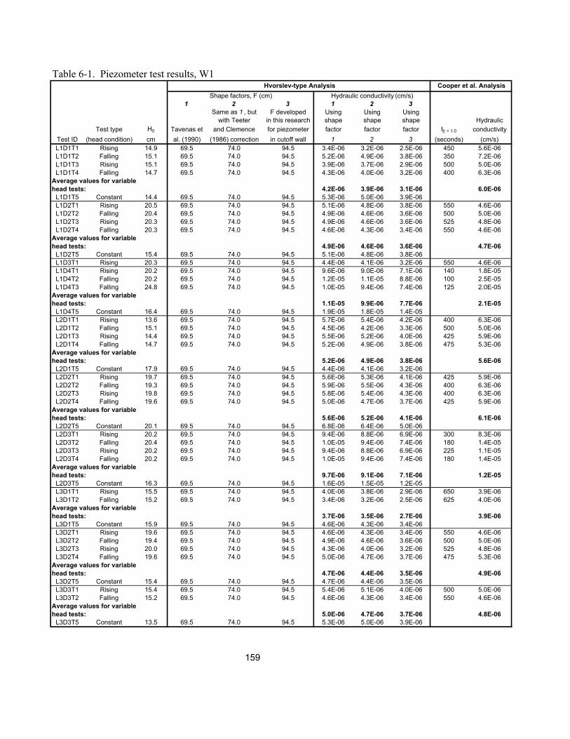
Table 6-1. Piezometer test results, W1

1 2 3 1 2 3Same as 1 , but F developed Using Using Using

with Teeter in this research shape shape shape HydraulicTest type H0 Tavenas et and Clemence for piezometer factor factor factor tβ = 1.0 conductivity

Test ID (head condition) cm al. (1990) (1986) correction in cutoff wall 1 2 3 (seconds) (cm/s)L1D1T1 Rising 14.9 69.5 74.0 94.5 3.4E-06 3.2E-06 2.5E-06 450 5.6E-06L1D1T2 Falling 15.1 69.5 74.0 94.5 5.2E-06 4.9E-06 3.8E-06 350 7.2E-06L1D1T3 Rising 15.1 69.5 74.0 94.5 3.9E-06 3.7E-06 2.9E-06 500 5.0E-06L1D1T4 Falling 14.7 69.5 74.0 94.5 4.3E-06 4.0E-06 3.2E-06 400 6.3E-06

Average values for variablehead tests: 4.2E-06 3.9E-06 3.1E-06 6.0E-06

L1D1T5 Constant 14.4 69.5 74.0 94.5 5.3E-06 5.0E-06 3.9E-06L1D2T1 Rising 20.5 69.5 74.0 94.5 5.1E-06 4.8E-06 3.8E-06 550 4.6E-06L1D2T2 Falling 20.4 69.5 74.0 94.5 4.9E-06 4.6E-06 3.6E-06 500 5.0E-06L1D2T3 Rising 20.3 69.5 74.0 94.5 4.9E-06 4.6E-06 3.6E-06 525 4.8E-06L1D2T4 Falling 20.3 69.5 74.0 94.5 4.6E-06 4.3E-06 3.4E-06 550 4.6E-06


L1D2T5 Constant 15.4 69.5 74.0 94.5 5.1E-06 4.8E-06 3.8E-06L1D3T1 Rising 20.3 69.5 74.0 94.5 4.4E-06 4.1E-06 3.2E-06 550 4.6E-06L1D4T1 Rising 20.2 69.5 74.0 94.5 9.6E-06 9.0E-06 7.1E-06 140 1.8E-05L1D4T2 Falling 20.2 69.5 74.0 94.5 1.2E-05 1.1E-05 8.8E-06 100 2.5E-05L1D4T3 Falling 24.8 69.5 74.0 94.5 1.0E-05 9.4E-06 7.4E-06 125 2.0E-05








L2D3T5 Constant 16.3 69.5 74.0 94.5 1.6E-05 1.5E-05 1.2E-05L3D1T1 Rising 15.5 69.5 74.0 94.5 4.0E-06 3.8E-06 2.9E-06 650 3.9E-06L3D1T2 Falling 15.2 69.5 74.0 94.5 3.4E-06 3.2E-06 2.5E-06 625 4.0E-06




L3D2T5 Constant 15.4 69.5 74.0 94.5 4.7E-06 4.4E-06 3.5E-06L3D3T1 Rising 15.4 69.5 74.0 94.5 5.4E-06 5.1E-06 4.0E-06 500 5.0E-06L3D3T2 Falling 15.2 69.5 74.0 94.5 4.6E-06 4.3E-06 3.4E-06 550 4.6E-06


L3D3T5 Constant 13.5 69.5 74.0 94.5 5.3E-06 5.0E-06 3.9E-06

159

Shape factors, F (cm) Hydraulic conductivity (cm/s)Hvorslev-type Analysis Cooper et al. Analysis

6.1.3.1 Hvorslev Analysis of Variable Head Tests – W1 Three shape factors were used for the Hvorslev analysis of the piezometer test results. The first was the shape factor from Tavenas et al. (1990) that is applicable to the ratio of filter length to diameter for the Geonor M206. This shape factor is 69.5 cm. The second shape factor incorporates the Teeter and Clemence (1986) correction factor that takes into account the close proximity of the trench walls. This shape factor is 74.0 cm (see Chapter 5). The third shape factor was obtained from Figure 5-14, which was developed by modeling a piezometer in a cutoff wall using the computer program MODFLOW, as described in Chapter 5. For the Geonor M206 piezometer in W1, this shape factor is 94.5 cm. Each of the three shape factors was used to evaluate the hydraulic conductivity of the wall in the Hvorslev-type analyses. For the variable head tests, the slope of the -ln(Ht/H0) versus time plot was evaluated in the range 0.1 ≤ Ht/H0 ≤ 0.3. Plots of -ln(Ht/H0) versus time for each variable head test are shown in Appendix A. Figure 6-3 shows plots for the variable head tests at L2D2. The plots are similar for each of the four tests, which, according to Butler (1996), indicates the absence of a "dynamic" low-k skin, which is the portion of a skin that would be mobilized by seepage forces in the tests2. Figure 6-4 shows the influence of flow direction on the variable head test results. Each point in the figure represents data from a single testing location in the wall (there is no point for L1D3 because only a single rising head test was performed here). The figure shows that flow direction had no significant impact on the estimated hydraulic conductivity. Finally, for each set of variable head tests at each testing point in the wall, the average value of hydraulic conductivity was calculated and is shown in bold in Table 6-1. 6.1.3.2 Hvorslev Analysis of Constant Head Tests – W1

Measurements in the constant head tests were made until the flow rate reached steady state. Plots of water volume flowing out of the piezometer versus time for each constant head test are shown in Appendix A. The same three shape factors used in the Hvorslev analysis of the variable head tests were used in the Hvorslev analysis of the constant head tests. The values of hydraulic conductivity for each shape factor are shown in Table 6-1.

2 Low-k skins are discussed in more detail in Subsection 6.3.3.1 for W3.

160

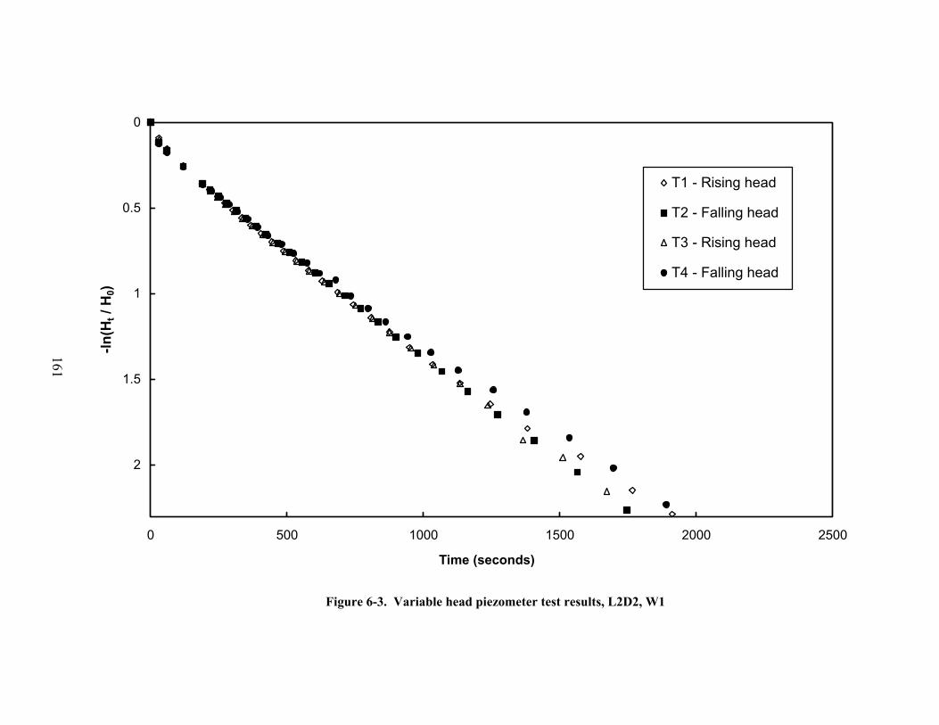
Figure 6-3. Variable head piezometer test results, L2D2, W1

0

0.5

1

1.5

2

0 500 1000 1500 2000 2500

Time (seconds)

-ln(H

t / H

0)

T1 - Rising head

T2 - Falling head

T3 - Rising head

T4 - Falling head

161

Figure 6-4. Effect of flow direction in variable head piezometer tests, W1

1.0E-06

1.0E-05

1.0E-06 1.0E-05k from rising head tests (cm/s)

k fr

om fa

lling

hea

d te

sts

(cm

/s)

k evaluated from Hvorslev-type analysiswith shape factor = 94.5 cm

162

6.1.3.3 Cooper et al. Analysis of Variable Head Tests – W1 The analysis procedure of Cooper et al. (1967) was also used to reduce the variable head test results. By plotting Ht/H0 versus log time for each test, the value of time at β = 1 (tβ = 1) was found from the curve fitting procedure. These times are shown in Table 6-1. The dimensionless parameter β is defined as: β = transmittivity × t / rc

2 (6-2) where t is time and rc is the radius of the standpipe. By setting β = 1 and t = tβ = 1, the transmittivity can be determined. For a partially penetrating well, the hydraulic conductivity may be evaluated as transmittivity divided by the length of the well filter. Values of hydraulic conductivity from the Cooper et al. method, including application of the Hyder et al. (1994) correction factor, are shown in Table 6-1. Average values for each testing location are shown in bold. The rest of this subsection goes into more detail on application of the Cooper et al. method and the Hyder et al. correction factor. There are type curves for different values of α in the Cooper et al. curve fitting method, where: α = γw mv rw

2 L / rc2 (6-3)

In Eq. 6-3, γw is the unit weight of water, mv is the coefficient of volume compressibility of the soil, rw is the radius of the filter, L is the filter length, and rc is the radius of the piezometer standpipe. Theoretically, matching the actual data to a type curve for a given α yields both the transmissivity (which may be taken as hydraulic conductivity times filter length) and the compressibility of the soil (evaluated by rearranging Eq. 6-3). However, Cooper et al. (1967) note that small shifts in the curve matching have a big impact on the estimated compressibility, but a relatively smaller impact on the estimated hydraulic conductivity. They suggest, if possible, to use other information to estimate a representative value of α, and to use this value of α in the curve fitting. The values of α determined from the curve fitting for the piezometer test data in this research varied significantly. Instead of accepting the values of α determined from the curve fitting, it was decided to estimate α from other information, as described below, and use this value of α in the curve fitting to evaluate hydraulic conductivity. The governing differential equation in the Cooper et al. method is the radial consolidation equation. As a result, the value of mv was related to the radial effective stress by the piezometer. Installing the piezometer in a cutoff wall increases the radial effective stress above the initial horizontal effective stress. Radial effective stresses can be estimated using the Bjerrum et al. (1972) approach discussed in Chapter 5. The following expression was used to estimate the coefficient of volume compressibility: mv = RR/2.3/σr', where RR is the recompression ratio measured in the 1D consolidation tests described in Chapter 4. The recompression ratio, as opposed to the virgin compression ratio, was used for the following reason. Before initiation of the first variable head test, the radial effective stress was on the virgin compression curve, because the radial

163

effective stress had increased above past values due to insertion of the piezometer. After the first variable head test, however, which was always a rising head test, subsequent volume changes, due to both falling and rising head tests, occurred on the unload/reload curve, which is represented by the recompression ratio.

For the piezometer tests in W1, application of the above approach resulted in a value of α of 5 × 10-3. This value was used in the curve fitting procedure to find the time at β = 1.

The Hyder et al. (1994) correction factor was applied to account for the vertical flow to/from the piezometer. For determination of this factor, the hydraulic conductivity of the soil-bentonite was assumed to be isotropic (this assumption will be supported in Section 6.4). For a piezometer radius to filter length ratio of 0.055 and a value of α = 5 × 10-3, the correction factor is approximately 1.5. This correction factor is the ratio of the hydraulic conductivity estimated by the Cooper et al. method (radial flow only) to the hydraulic conductivity considering both radial and vertical flow. Finally, it is noted that the curve fitting was not straight-forward for the piezometer test data in this research. The shapes of the data curves for all the tests were such that the values of α determined from the curve fitting varied significantly, and in some cases, a good curve fit was not possible. When a single, representative value of α was estimated and used in the curve fitting, determination of the times at β = 1 was very subjective due to the different shapes of the data curves compared to the theoretical curve for the estimated α. 6.1.3.4 Comparison of Piezometer Test Analysis Methods – W1

Hvorslev hydraulic conductivity values from the constant head tests are compared

to Hvorslev values from the variable head tests in Figure 6-5. The variable head hydraulic conductivity value used in the figure is the average value from all the variable head tests at a single testing point in the wall. Excluding the tests at L1D4 and L2D3, there was good agreement between the constant head and variable head tests, with the constant head values (excluding L1D4 and L2D3) approximately 10% higher, on average, than the variable head values. Tremblay and Eriksson (1987) noticed a similar trend when comparing constant and variable head tests, with constant head results approximately 20% higher than variable head results. For the tests at L1D4 and L2D3, which yielded higher hydraulic conductivities, the constant head values were approximately 75% higher, on average, than the variable head values. A possible explanation for this is that the sustained seepage forces in the constant head tests caused migration of bentonite through the relatively larger pores in the soil near the filter at these higher-k locations which further increased the hydraulic conductivity of the soil above that measured in the variable head tests, where the seepage forces were not maintained but dissipated with time. Although this explanation seems reasonable, it is only speculation; the relationships between seepage forces (magnitude and duration of time applied), pore sizes, and migration of bentonite are not known.

164

Figure 6-5. Comparison of variable and constant head piezometer test results, W1

1.0E-06

1.0E-05

1.0E-04

1.0E-06 1.0E-05 1.0E-04k from variable head tests (cm/s)

k fr

om c

onst

ant h

ead

test

s (c

m/s

)

k evaluated from Hvorslev-type analysiswith shape factor = 94.5 cm

L1D4 and L2D3

165

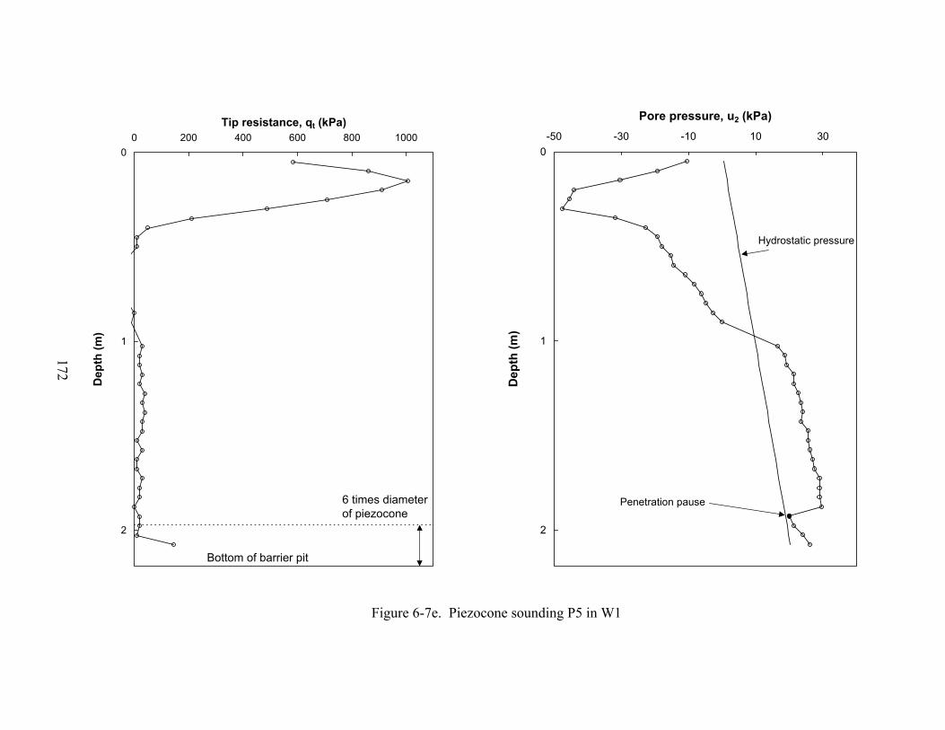
The results of the variable head tests evaluated using the Hvorslev analysis (with shape factor = 94.5 cm) are compared to the results evaluated using the Cooper et al. analysis in Figure 6-6. As seen in the figure, the Cooper et al. values are higher than the Hvorslev values. The difference may be partly due to the fact that the Cooper et al. analysis does not account for the close proximity of the trench walls3. This can be seen by comparing the Cooper et al. values to the Hvorslev values evaluated using the Tavenas et al. shape factor of 69.5 cm, which does not account for the trench walls. As seen in Table 6-1, these values are much closer to each other than the values presented in Figure 6-6. The best estimate of hydraulic conductivity from the piezometer tests is obtained by reducing the data using the Hvorslev-type analysis with the shape factor from Figure 5-14 that takes into account the close proximity of the trench walls. Using the shape factor from Tavenas et al. leads to overestimating hydraulic conductivity by 36%, and using the Tavenas et al. shape factor with the Teeter and Clemence correction factor leads to overestimating hydraulic conductivity by 28%. The Cooper et al. analysis also overestimates hydraulic conductivity because, for one known reason, it does not account for the close trench walls. When comparing measures of hydraulic conductivity in Section 6.1.6, the values in Table 6-1 for the Hvorslev-type analysis with shape factor = 94.5 cm will be used. 6.1.4 Piezocone Soundings – W1 Figure 6-2 shows six locations in W1 where the piezocone was used to probe the cutoff wall. The soundings are labeled P1 through P6 (Push 1, Push 2, etc.). In addition, the piezocone was pushed into the compacted LCS on one side of the cutoff wall at P7. Figure 6-2 also shows the locations of five pore pressure dissipation tests. The following two subsections discuss the piezocone profiles and pore pressure dissipation tests. 6.1.4.1 Piezocone Profiles of W1 Figure 6-7 shows the measured tip resistance and pore pressure (in the number 2 position) for the soundings. The measured sleeve friction was essentially zero. The hydrostatic pore pressure is plotted in the pore pressure plots. Penetration pauses are shown by solid circles. Penetration pauses were for addition of push-rods or dissipation tests.

3 The boundary condition used in the Cooper et al. (1967) method has the excess head equal to zero at an infinite radial distance from the piezometer. The nearby trench walls cause the excess head to be zero at a finite distance from a piezometer in a cutoff wall: the distance between the piezometer and the trench wall.

166

Figure 6-6. Comparison of variable head piezometer test results from Hvorslev-type and Cooper et al. analyses, W1

1.0E-06

1.0E-05

1.0E-04

1.0E-06 1.0E-05 1.0E-04k from Hvorslev-type analysis (cm/s)

k fr

om C

oope

r et a

l. an

alys

is (c

m/s

)

For k evaluated from Hvorslev-typeanalysis, shape factor = 94.5 cm

167

0

1

2

-40 -20 0 20 40

Pore pressure, u2 (kPa)

Dep

th (m

)

Hydrostatic pressure

Penetration pause

0

1

2

0 100 200 300 400 500 600Tip resistance, qt (kPa)

Dep

th (m

)

Bottom of barrier pit

6 times diameterof piezocone

168

Figure 6-7a. Piezocone sounding P1 in W1

0

1

2

-40 -20 0 20 40


Dep

th (m

)


Penetration pause

0

1

2

0 100 200 300 400 500Tip resistance, qt (kPa)

Dep

th (m

)



169

Figure 6-7b. Piezocone sounding P2 in W1

0

1

2

-40 -20 0 20 40


Dep

th (m

)


Penetration pause

0

1

2


Dep

th (m

)



170

Figure 6-7c. Piezocone sounding P3 in W1

0

1

2

-40 -20 0 20 40


Dep

th (m

)


Penetration pause

0

1

2


Dep

th (m

)



171

Figure 6-7d. Piezocone sounding P4 in W1

0

1

2

-50 -30 -10 10 30


Dep

th (m

)


Penetration pause

0

1

2


Dep

th (m

)



172

Figure 6-7e. Piezocone sounding P5 in W1

0

1

-50 -30 -10 10 30


Dep

th (m

)


Penetration pause

0

1

0 200 400 600 800Tip resistance, qt (kPa)

Dep

th (m

)



173

Figure 6-7f. Piezocone sounding P6 in W1

0

1

2

-40 -20 0 20 40


Dep

th (m

)


0

1

2


Dep

th (m

)



174

Figure 6-7g. Piezocone sounding P7 in compacted LCS

As a representative sounding in the cutoff wall, consider P3 in Figure 6-7c. Within about the top 0.4 m, the relatively high tip resistances and negative pore pressures are evidence of a desiccated crust. Down to about 2.4 m, the measurements are indicative of intact soil-bentonite, with tip resistance of about 125 kPa and excess pore pressure (the pore pressure above hydrostatic) of about 10 kPa. For comparison, at the Gilson Road site discussed in Chapter 2, the intact soil-bentonite gave an average tip resistance of 147 kPa and an average excess pore pressure of roughly 10 kPa (Barvenik and Ayres, 1987). When the piezocone reached a depth of about 2.4 m, the excess pore pressure went to zero and the tip resistance jumped to about 300 kPa (4). This type of response indicates penetration into a different, stronger, higher permeability material. A LCS defect was found at the bottom of the wall during destructive evaluation. The piezocone measurements at this depth—relatively higher tip resistance and approximately zero excess pore pressure—indicate this defect. For comparison, at the Gilson Road site, measured tip resistances ranged from about 400 to 1900 kPa for what was described as a "low density clean granular window." (The stresses on their windows in the wider wall were likely higher than the very low stresses on the defect at the bottom of the 30.5-cm-wide W1.) There are two important notes related to P2, P4, and P5. At the locations of P2 and P4, the top of the cutoff wall was excavated and replaced with fill material (combination of LCS and soil-bentonite) prior to the piezocone soundings. The depths of excavation and replacement were approximately 0.4 m for P2 and 0.8 m for P4. The response of the piezocone in these areas is representative of the fill, and not the cutoff wall. For P5, it was observed after the piezocone was removed from the wall that the tip of the cone was loose. This may account for the unusually low tip resistance measurements for this sounding. Figure 6-7g shows the piezocone sounding in the compacted LCS adjacent to the cutoff wall. As can be seen, the tip resistance is much higher than in the soil-bentonite, and no excess pore pressure was generated due to the high hydraulic conductivity of the LCS. All of the cutoff wall soundings in Figure 6-7 show results similar to those found in P3 described above. The defect at the bottom of the wall was detected by P1, P2, P3, and P4. Figure 6-2 shows the depths where the piezocone indicated the defect. As can be seen in the figure, there is good agreement between where the piezocone indicated the defect and where the defect was observed during destructive evaluation. This finding can be generalized to all three zones in the cutoff wall: desiccated top, intact soil-bentonite, and defect at the bottom. By comparing the piezocone soundings to the observed materials in the wall, it was found that the piezocone provided a clear picture of the materials comprising the cutoff wall.

4 Increases in tip resistance within approximately 6 times the diameter of the piezocone from the bottom of the barrier pit are assumed to be due to the influence of the concrete bottom of the pit.

175

6.1.4.2 Pore Pressure Dissipation Tests The results of five pore pressure dissipation tests are shown in Table 6-2. The locations of the dissipation tests in the cutoff wall are shown in Figure 6-2. For each dissipation test, the excess pore pressure, ue, was plotted versus the square root of time, as shown for the dissipation test in P6 in Figure 6-8 (plots for the other four dissipation tests are given in Appendix B). For each test, Table 6-2 shows the time required for 50% of the excess pore pressure to dissipate, t50. Two methods were used to evaluate hydraulic conductivity from the dissipation tests: 1) Parez and Fauriel (1988), Eq. 5-27 and 2) Baligh and Levadoux (1980), Eq. 5-29. For use in the Baligh and Levadoux approach, the coefficient of consolidation in the horizontal direction, ch, was evaluated using the Houlsby and Teh (1988) piezocone model. See Chapter 5 for a description of these methods. For both methods of evaluating hydraulic conductivity, the results of the five tests are quite consistent. The average values are 1.9 × 10-6 cm/s from Eq. 5-27 and 3.1 × 10-6 cm/s from Eq. 5-29. The values from Eq. 5-29 are believed to be more accurate due to the more approximate nature of Eq. 5-27.

While there is certainly a component of vertical flow in the dissipation tests, the estimated value of hydraulic conductivity is closer to the horizontal hydraulic conductivity of the cutoff wall. From a study on pore pressure dissipation in piezocone tests, Baligh and Levadoux (1986) concluded that pore pressure dissipation is predominantly in the horizontal direction. Table 6-2. Results of piezocone dissipation tests – W1

Push number

Depth (m) t50 (s) k (cm/s) Eq. 5-27

ch (1) (cm2/s)

Eq. 5-28

σv0' (2) (kPa)

k (3) (cm/s) Eq. 5-29

P1 1.55 156 1.8 × 10-6 0.086 2.66 3.0 × 10-6 P2 2.20 171 1.6 × 10-6 0.079 2.68 2.8 × 10-6 P3 2.08 138 2.1 × 10-6 0.097 2.68 3.4 × 10-6 P5 1.93 135 2.2 × 10-6 0.100 2.68 3.5 × 10-6 P6 1.05 163 1.7 × 10-6 0.082 2.58 3.0 × 10-6

Notes: (1) T* = 0.245, r = 1.78 cm, and Ir = 300. (2) Calculated using arching theory. (3) RR = 0.0022. Finally, note that the hydraulic conductivities estimated from the tests in P2 and P5 are consistent with the other dissipation test values, despite the close proximity of the defect to these two testing locations. This indicates the small zone of measurement in the vertical direction and the dominance of horizontal flow in the tests.

176

Figure 6-8. Dissipation test data for P6 in W1

-2

0

2

4

6

8

10

12

14

16

0 1 2 3 4

Square root of time (minutes^0.5)

u e (k

Pa)

177

6.1.5 Lab Tests on Undisturbed Samples – W1 The hydraulic conductivities of two undisturbed samples taken from W1 during destructive evaluation were measured according to the procedure described in Chapter 5. The locations of the samples in the wall are shown in Figure 6-2. Both samples were obtained such that the vertical hydraulic conductivity of the soil-bentonite was measured. Table 6-3 shows the measured hydraulic conductivity values, as well as the initial water contents, lengths of the samples, and effective surcharge pressures applied above the samples. Table 6-3. Hydraulic conductivity of undisturbed samples – W1 Sample

ID Sample

orientation Initial water

content(1) (%)

Length of sample (cm)

Effective surcharge

(kPa)

Hydraulic conductivity

(cm/s) W1U1 Vertical 28.1 2.6 1.5 2.0 × 10-6 W1U2 Vertical 29.8 2.5 1.6 2.3 × 10-6

Notes: (1) Measured from soil-bentonite in cutoff wall in vicinity of undisturbed sample. 6.1.6 Comparisons – W1 Table 6-4 compares the results of the four types of hydraulic conductivity tests performed for W1. The following paragraphs compare the methods in detail. Table 6-4 lists the direction of hydraulic conductivity that was measured in each test. In the API tests, the major principal consolidation stress was in the same direction as the measured hydraulic conductivity, which is analogous to measuring the vertical hydraulic conductivity in the pilot-scale walls, where the arching mechanism controls and the vertical stress is the major principal stress. In contrast, both the piezometer tests and the piezocone dissipation tests measure predominantly the horizontal hydraulic conductivity. Finally, only the vertical hydraulic conductivity of the undisturbed samples was measured for W1. It is often important to relate hydraulic conductivity to consolidation stress. For the soil-bentonite used in this research, it is convenient to relate hydraulic conductivity to preconsolidation stress, since changes in void ratio, and therefore hydraulic conductivity, are small during unload and reload of stress. In fact, the hydraulic conductivity is not even very sensitive to virgin compression in the stress range used in this research, as seen, for example, by the results of the API tests on grab samples. Table 6-4 shows the consolidation stresses controlling each measure of hydraulic conductivity. For the API tests, the consolidation stress is the gross effective pressure, which increased from 5.6 to 9.0 kPa as the air pressure in the tests increased from 6.9 to 13.8 kPa. For the piezometer tests, the consolidation stress controlling the hydraulic conductivity was assumed to be the radial effective stress near the piezometer after installation. An estimate of this stress,

178

possibly on the low end of a reasonable range of values, is 11 kPa, estimated using the Bjerrum et al. (1972) method in Chapter 5. A conservative approach was taken in Chapter 5 to estimate a low value of radial effective stress in the prediction of hydraulic fracture pressures. For piezocone dissipation tests, Baligh and Levadoux (1986) concluded that consolidation occurs predominantly on the recompression curve for degrees of dissipation less than 50%. Since the shapes of the dissipation curves up to 50% dissipation were used to evaluate hydraulic conductivity from the dissipation tests, the preconsolidation stress in the wall prior to installation of the piezocone was used as the stress controlling hydraulic conductivity. For the depths of the dissipation tests, this stress ranged from 9 to 10 kPa. The preconsolidation stress in the wall was also used for the lab tests on undisturbed samples. At the depth of sampling, this stress, 7 kPa, was greater than the effective surcharge pressures of 1.5 and 1.6 kPa applied to the samples during testing. Finally, it is noted that the range of preconsolidation stresses in the wall (vertical effective stresses) where the in situ hydraulic conductivity tests were performed was 7 to 10 kPa. Because the range of stresses applicable to all of the tests is not large, and the hydraulic conductivity of this particular soil-bentonite is rather insensitive to changes in stress in this range, consolidation stress may be dismissed as a factor differentiating the hydraulic conductivity results. Table 6-4. Comparison of hydraulic conductivity measurements for W1 Hydraulic conductivity test

Average hydraulic conductivity

(cm/s)


direction

Consolidation stress controlling

k (kPa)

Sample size

API tests on grab samples

1.3 × 10-6 Vertical 5.6 to 9.0 220 cm3

Piezometer tests(1)

3.5 × 10-6 Predominantly horizontal

11 Between 10,000 and 45,000 cm3

Piezocone dissipation tests(2)


9 to 10 Roughly 1,000 to

2,000 cm3 Lab tests on undisturbed samples

2.2 × 10-6 Vertical 7 110 cm3

Notes: (1) From variable head tests. Not including measurements at L1D4 and L2D3 influenced by defect. See Section 6.4 for evaluation of sample size for piezometer tests. (2) Sample size estimated using piezocone model in Chapter 4 of Burns and Mayne (1998), which is based on radial consolidation and a plasticized zone of radius rcone Ir

0.333 beyond which no ue is generated. Table 6-4 also provides a sample size for each test. The lab tests on both remolded and undisturbed samples probe the smallest volume of material, the piezometer tests probe the largest volume, and the piezocone dissipation tests probe an intermediate volume (the most uncertainty is in the volume tested by the piezocone). The following evidence supports the larger zone of measurement in the piezometer tests compared to the

179

piezocone dissipation tests. Piezometer tests at L1D4 and L2D3 were influenced by the defect at the bottom of the wall; the measured hydraulic conductivities were slightly over 2 times higher than the average value measured in the rest of the wall. However, the dissipation tests in P2 and P5, which were just as close or closer to the defect than the piezometer tests at L1D4 and L2D3, did not appear to be influenced by the defect. The standard deviations of the negative logarithm of the hydraulic conductivity values from the six API tests, eight piezometer test locations (excluding the two locations influenced by the defect), and five piezocone dissipation tests were 0.03, 0.06, and 0.04, respectively. These values are well below the typical range of 0.2 to 0.3 for lab tests on soil-bentonite from real cutoff walls (see Chapter 7), which is presumably due to the higher degree of soil-bentonite mixing and smaller degree of variability in the base soil in the soil-bentonite for W1. Because the numbers of samples corresponding to the standard deviations reported above are not very big, it is not advisable to compare them in great detail. In Section 6.4, after the results from all three cutoff walls are compared, the reasons for the differences in the values from the various types of tests will be discussed.

180

6.2 Hydraulic Conductivity Test Results for W2 This section has the following parts: 6.2.1 API Tests on Grab Samples – W2 6.2.2 Global Measurement of Average Hydraulic Conductivity – W2 6.2.3 Piezometer Tests – W2 6.2.4 Piezocone Soundings – W2 6.2.5 Lab Tests on Undisturbed Samples – W2 6.2.6 Comparisons – W2 6.2.1 API Tests on Grab Samples – W2 The results of the API tests on the grab samples from W2 are shown in Figure 6-9. As with W1, the hydraulic conductivity values are not significantly dependent on consolidation pressure in the range of pressures applied. The consolidation pressures in the tests, calculated using Eq. 6-1, were 5.6 and 9.0 kPa. For all six samples, the average hydraulic conductivities corresponding to the pressures 5.6 and 9.0 kPa were 2.0 × 10-6 and 2.1 × 10-6 cm/s, respectively. Under application of the first consolidation pressure, vertical strains from –3% to –5% were measured in the specimens. However, as with the samples from W1, the strains were negligible between the consolidation pressures 5.6 and 9.0 kPa.

The standard deviations of the negative logarithm of the hydraulic conductivity values for consolidation pressures 5.6 and 9.0 kPa are 0.08 and 0.09, respectively. These values are higher than those for W1, but are approximately one-third the magnitude of typical values for real soil-bentonite cutoff walls. 6.2.2 Global Measurement of Average Hydraulic Conductivity – W2 The average hydraulic conductivity of W2 was measured using the four water level pairs shown in Table 5-1. Because of the relatively high flow rates through the wall, flow rates into/out of the wells at A and B on the upgradient side (see Figure 5-2) were not measured; water was simply added to the well at B and removed from the well at A to maintain the upgradient water level. For each water level pair, the first step was to measure the background flow rate on the downgradient side, qDG,b.g. (Eq. 5-2b), with the water levels on each side of the wall at the eventual downgradient level (no gradient across the wall). These background flow rates are shown in Table 6-5.

181



10

Hyd

raul

ic c

ondu

ctiv

ity (c

m/s

)

1e-6

1e-5

Sample 1 32.5 26.7Sample 2 31.7 26.5Sample 3 30.8 26.5Sample 4 33.5 26.5Sample 5 32.0 26.0Sample 6 31.8 25.7

4 14


Sample 5

Sample 3

182

Next, the water level on the eventual upgradient side was raised to the upgradient level, and the flow rate into the well at D, qD, was measured. Due to the high flow rates through the wall, it was not necessary to add water into the well at C. The measured values of qD for each water level pair are shown in Table 6-5. The flow rates through the wall, qw, were calculated using Eq. 5-3b. These values are shown in Table 6-5. For each water level pair, it took only approximately one day to measure the flow rate through the wall, because the total flow rate was dominated by flow through the defects, and these flow rates reached steady state quickly. Table 6-5. Flow rates through W2 during global average hydraulic conductivity measurements

Water level pair qDG,b.g. (cm3/s) qD (cm3/s) qw (cm3/s) 1 -0.29 0.79 0.50 2 0.11 0.87 0.98 3 0.20 0.99 1.18 4 0.56 0.85 1.41

The average hydraulic conductivities of the wall corresponding to the above flow rates were calculated using Eq. 5-9 and the shape factors from Flow model 3 in Table 5-2. These hydraulic conductivities, shown in Table 6-6, are average values for the height of the wall ranging from approximately the elevation of the downgradient water level to the bottom of the barrier pit. Table 6-6. Average hydraulic conductivities from flow rates measured through W2

Water level pair Hydraulic conductivity (cm/s) 1 9.9 × 10-5 2 9.9 × 10-5 3 7.9 × 10-5 4 6.1 × 10-5

From the flow rate measurements shown in Table 6-5, the average hydraulic conductivities of Layers A through D (shown in Figure 5-3 and Figure 6-10) were evaluated using Flow model 3 in the procedure outlined in Section 5.2.2, Chapter 5. These values are shown in Table 6-7. Table 6-7. Average hydraulic conductivities of Layers A through D in W2

Layer Hydraulic conductivity (cm/s) A 9.9 × 10-5 B 9.9 × 10-5 C 3.0 × 10-5 D 2.5 × 10-5

183

Figure 6-10. Hydraulic conductivity test locations, W2

CCL

Fill Fill

LCS defectbelow dottedline

Cutoff wall boundaries

Soil-bentonite

W2U5W2U4

W2U3

W2U1, W2U2

W2U6

Undisturbed samples

2 meters

L1D1

L1D2

L1D3L2D3

L3D1

L3D2

Piezometer tests

Layer D

Layer C

Layer B

Layer A

Layers in soil-bentonitewhere average hydraulicconductivity was measuredusing i = 0.25

184

6.2.3 Piezometer Tests – W2 Figure 6-10 shows the places in W2 where piezometer tests were performed using the Geonor M206 piezometer. Piezometer tests were performed at six points in the wall. The results of the piezometer tests are shown in Table 6-8. The format of Table 6-8 is the same as that of Table 6-1 for W1. The two hydraulic fracture tests in W2 were performed at L1D3 and L3D2 after the hydraulic conductivity tests were completed at these points. 6.2.3.1 Hvorslev Analysis of Variable Head Tests – W2 Three shape factors were used for the Hvorslev-type analysis of the variable head piezometer test results. The first was the shape factor from Tavenas et al. (1990) that is applicable to the ratio of filter length to diameter for the Geonor M206. This shape factor is 69.5 cm. The second shape factor incorporates the Teeter and Clemence (1986) correction factor that takes into account the close proximity of the trench walls. As discussed in Section 5.3.2.1, Chapter 5, this correction factor is 1 for a 61-cm-wide wall. The third shape factor was obtained from Figure 5-14, which was developed in this research for piezometer tests in cutoff walls. For the Geonor M206 piezometer in W2, this shape factor is 81.0 cm. Values of hydraulic conductivity evaluated from the Hvorslev-type analysis are shown in Table 6-8. Average values for the tests are shown in bold. The data used for these analyses are presented in Appendix A in the form of plots of -ln(Ht/H0) versus time. The behavior of the variable head tests was similar to those for W1 with respect to repeatability and flow direction; repeat tests at a given location produced similar plots of -ln(Ht/H0) versus time and flow direction had no significant impact on hydraulic conductivity. The exception was the test series at L3D1. The plots of -ln(Ht/H0) versus time were significantly different for the four variable head tests performed at this location, and the k values for the rising head tests were significantly higher than the k values for the falling head tests. This may be evidence of a low-k skin of dynamic nature for this location5. At any rate, the accuracy of the results for this location is questionable. It appears that the piezometer test results for L1D1 and L1D2 were representative of defect-free soil-bentonite in the wall. The test results for L1D3, L2D3, and L3D2, however, appear to be representative of a higher-hydraulic-conductivity material, perhaps due to a reduction in bentonite content from flushing by the bioslurry as hypothesized in Section 4.9.1.2 in Chapter 4. Also, the tests at L1D3 and L2D3 may have been close enough to the defects in the wall to have had the defects influence the measurements. (Recall that there was sand at the soil-bentonite/CCL interface above the dotted line shown in Figure 6-10 that was fairly close to these locations.)

5 Low-k skins are discussed in more detail in Subsection 6.3.3.1 for W3.

185




Test ID (head condition) cm al. (1990) (1986) correction in cutoff wall 1 2 3 (seconds) (cm/s)L1D1T1 Rising 15.0 69.5 69.5 81.0 7.6E-06 7.6E-06 6.5E-06 175 1.4E-05L1D1T2 Falling 15.8 69.5 69.5 81.0 4.8E-06 4.8E-06 4.1E-06 175 1.4E-05L1D1T3 Rising 15.3 69.5 69.5 81.0 5.7E-06 5.7E-06 4.9E-06 200 1.3E-05L1D1T4 Falling 15.4 69.5 69.5 81.0 6.2E-06 6.2E-06 5.3E-06 175 1.4E-05












L3D2T5 Constant 15.2 69.5 69.5 81.0 1.8E-05 1.8E-05 1.5E-05

186


6.2.3.2 Hvorslev Analysis of Constant Head Tests – W2 Measurements in the constant head tests were run until steady state was reached. Plots of water volume flowing out of the piezometer versus time for each constant head test are shown in Appendix A. The same three shape factors used in the Hvorslev analysis of the variable head tests were used in the Hvorslev analysis of the constant head tests. The values of hydraulic conductivity for each shape factor are shown in Table 6-8. 6.2.3.3 Cooper et al. Analysis of Variable Head Tests – W2 Table 6-8 also shows the results of the Cooper et al. (1967) analysis procedure for hydraulic conductivity. The value of α used in the curve fitting was 3 × 10-3, evaluated using the same approach as for W1. A Hyder et al. (1994) correction factor of 1.5 was used for W2 (there is not much difference between correction factors at α = 5 × 10-3 (W1) and α = 3 × 10-3, and it is difficult to distinguish this difference from the chart provided by Hyder et al. for this correction factor). 6.2.3.4 Comparison of Piezometer Test Analysis Methods – W2

For locations L1D1 and L1D2 in defect-free soil-bentonite, the Hvorslev constant head results were approximately 31% higher, on average, than the Hvorslev variable head results. For the tests in higher-hydraulic-conductivity materials at L1D3, L2D3, and L3D2, the Hvorslev constant head results were approximately 73% higher, on average, than the Hvorslev variable head results. The relatively higher constant head results at L1D3, L2D3, and L3D2 may be due to the same mechanism hypothesized in Subsection 6.1.3.4 for tests in low versus high k materials in W1. For L3D1, where the accuracy of the results is questionable, the constant head value was 116% higher than the variable head value.

Also, similarly to W1, the Cooper et al. variable head results were higher than the

Hvorslev variable head results evaluated using the shape factor for piezometer tests in cutoff walls developed in this research (81.0 cm). While this is partly due to the fact that the Cooper et al. method does not account for the close trench walls, there seem to be other factors involved, since the Cooper et al. results were also significantly higher than the Hvorslev results evaluated with the Tavenas et al. shape factor that does not account for the close trench walls. In general, there was less consistency between the Hvorslev constant head and variable head results, and the Hvorslev and Cooper et al. variable head results, than in W1. For comparison with other measures of hydraulic conductivity in Section 6.2.6, the variable head values in Table 6-8 from the Hvorslev analysis with shape factor = 81.0 cm will be used. Furthermore, only test results from L1D1 and L1D2 will be used.

187

6.2.4 Piezocone Soundings – W2 Unfortunately, attempts at probing W2 with the piezocone were not successful; the quality of data obtained from the soundings was poor. This may have been due to: 1) the piezocone becoming out of calibration from the time it was used in W1 and/or 2) baseline shifts during probing that were significant compared to the low loads from the soil-bentonite. The Hogentogler operating manual states that the amount of dirt migrating into the instrument and the amount of lubrication in the instrument can significantly affect the baselines. The exact reason for the poor data from the soundings in W2 was not discovered, and in order to stay within the time schedule for this research, it was decided to move on to the next phase of testing. 6.2.5 Lab Tests on Undisturbed Samples – W2 The hydraulic conductivities of six undisturbed samples taken from W2 during destructive evaluation were measured. The locations of the samples in the wall are shown in Figure 6-10. In order to investigate the anisotropy in the soil-bentonite hydraulic conductivity, a vertical sample and a horizontal sample were taken side by side at two different locations in the wall. Table 6-9 shows the measured hydraulic conductivity values, as well as the initial water contents, lengths of the samples, and effective surcharge pressures applied above the samples. Table 6-9. Hydraulic conductivity of undisturbed samples – W2 Sample

ID Sample


content(1) (%)


Effective surcharge

(kPa)


(cm/s) W2U1 Vertical 31.0 2.3 1.5 8.2 × 10-6 W2U2 Horizontal 31.0 3.6 1.5 1.3 × 10-5 W2U3 Horizontal 29.1 2.7 1.5 2.5 × 10-5 W2U4 Horizontal 29.1 2.3 1.5 4.6 × 10-6 W2U5 Vertical 29.1 2.8 1.5 4.0 × 10-6 W2U6 Horizontal 28.6 2.3 1.5 1.5 × 10-5

Notes: (1) Measured from soil-bentonite in cutoff wall in vicinity of undisturbed sample. 6.2.6 Comparisons – W2 Table 6-10 compares the results of the hydraulic conductivity tests performed for W2. The table shows the direction in which the hydraulic conductivity was measured, the consolidation stress controlling the hydraulic conductivity, and the approximate sample size. See Section 6.1.6 (Comparisons - W1) for discussions of these items. As with W1, consolidation stress may be dismissed as a factor differentiating the hydraulic conductivity results.

188

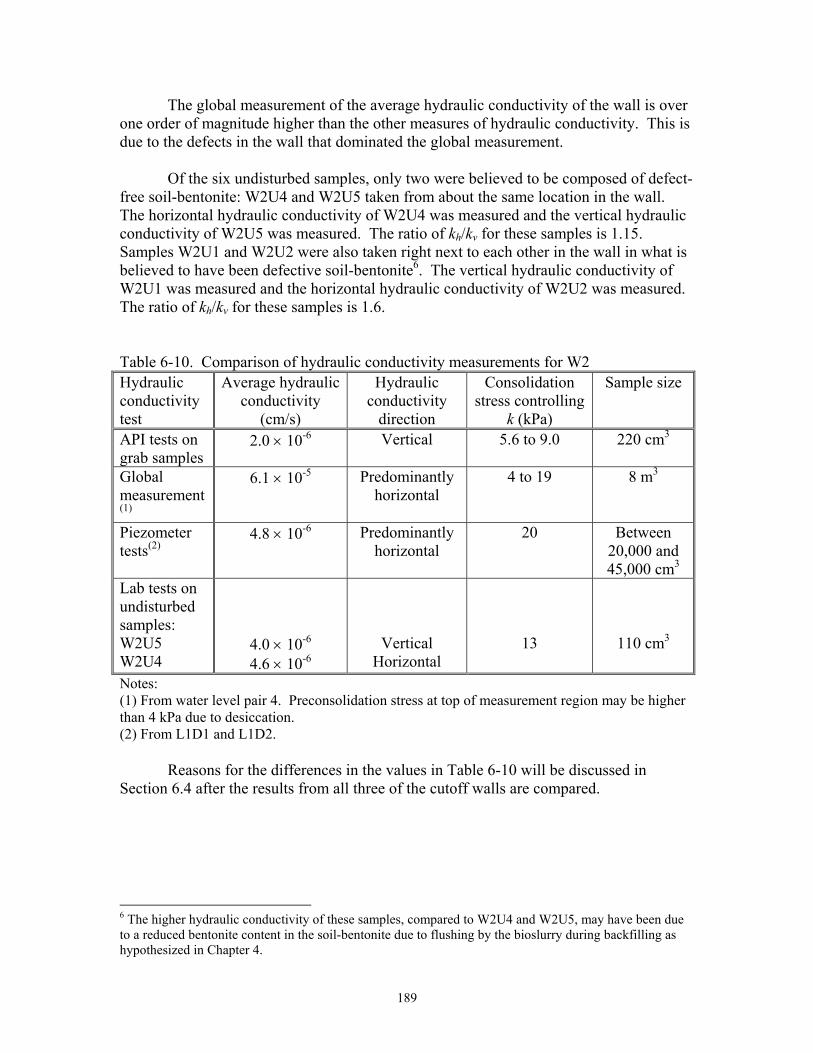
The global measurement of the average hydraulic conductivity of the wall is over one order of magnitude higher than the other measures of hydraulic conductivity. This is due to the defects in the wall that dominated the global measurement. Of the six undisturbed samples, only two were believed to be composed of defect-free soil-bentonite: W2U4 and W2U5 taken from about the same location in the wall. The horizontal hydraulic conductivity of W2U4 was measured and the vertical hydraulic conductivity of W2U5 was measured. The ratio of kh/kv for these samples is 1.15. Samples W2U1 and W2U2 were also taken right next to each other in the wall in what is believed to have been defective soil-bentonite6. The vertical hydraulic conductivity of W2U1 was measured and the horizontal hydraulic conductivity of W2U2 was measured. The ratio of kh/kv for these samples is 1.6. Table 6-10. Comparison of hydraulic conductivity measurements for W2 Hydraulic conductivity test


(cm/s)


direction


k (kPa)

Sample size


2.0 × 10-6 Vertical 5.6 to 9.0 220 cm3

Global measurement(1)


4 to 19 8 m3

Piezometer tests(2)


20 Between 20,000 and 45,000 cm3

Lab tests on undisturbed samples: W2U5 W2U4

4.0 × 10-6 4.6 × 10-6

Vertical Horizontal

13

110 cm3

Notes: (1) From water level pair 4. Preconsolidation stress at top of measurement region may be higher than 4 kPa due to desiccation. (2) From L1D1 and L1D2. Reasons for the differences in the values in Table 6-10 will be discussed in Section 6.4 after the results from all three of the cutoff walls are compared.

6 The higher hydraulic conductivity of these samples, compared to W2U4 and W2U5, may have been due to a reduced bentonite content in the soil-bentonite due to flushing by the bioslurry during backfilling as hypothesized in Chapter 4.

189

6.3 Hydraulic Conductivity Test Results for W3 This section has the following parts: 6.3.1 API Tests on Grab Samples – W3 6.3.2 Global Measurement of Average Hydraulic Conductivity – W3 6.3.3 Piezometer Tests – W3 6.3.4 Lab Tests on Undisturbed Samples – W3 6.3.5 Comparisons – W3 Due to the problem encountered in W2 with the piezocone, the high quality of data already obtained from W1, and time restrictions, the piezocone was not used to probe W3. 6.3.1 API Tests on Grab Samples – W3 The results of the API tests on the grab samples from W3 are shown in Figure 6-11. As with W1 and W2, the hydraulic conductivity values were not significantly dependent on consolidation pressure in the range of pressures applied. The consolidation pressures for samples 1 – 4 and 6, calculated using Eq. 6-1, were 5.6, 9.0, and 15.9 kPa. For these five samples, the average hydraulic conductivities corresponding to the above pressures were 1.0 × 10-7 (7), 1.1 × 10-7, and 1.3 × 10-7 cm/s, respectively. A smaller surcharge pressure was used for Sample 5 compared to the other five samples. The hydraulic conductivity of Sample 5 was 9.0 × 10-8 cm/s at 4.4 kPa. At higher pressures, fines were washed from the sample. Under application of the first consolidation pressure, vertical strains from –4% to –6% were measured in Samples 1 – 4 and 6. As with the samples from W1 and W2, the strains were negligible between the higher consolidation pressures.

The standard deviation of the negative logarithm of the hydraulic conductivity values for each consolidation pressure was in the range of 0.08 to 0.09. 6.3.2 Global Measurement of Average Hydraulic Conductivity – W3 Only one water level pair, producing a hydraulic gradient of 1, was applied to W3. The water level depths on the upgradient and downgradient sides were 30.5 and 91 cm, respectively. Subsection 6.3.2.1 discusses measurement of the flow rate through the wall and Subsection 6.3.2.2 discusses determination of its hydraulic conductivity.

7 The hydraulic conductivity value for Sample 4 was not used to calculate this average. See the note for this value in Figure 6-11.

190



10

Hyd

raul

ic c

ondu

ctiv

ity (c

m/s

)

1e-8

1e-7

1e-6

Sample 1 35.9 29.5Sample 2 36.0 29.0Sample 3 36.4 30.5Sample 4 34.4 29.1Sample 5 36.5 33.2*Sample 6 37.1 30.6

4 18


Graduated cylinder not sealed to atmosphere.Probably lost some discharge water to evaporation.Situation corrected at higher consolidation pressures.

* After erosion of fines at air pressure = 13.8 kPa.

191

6.3.2.1 Measurement of Flow Rate Through W3

Before application of the hydraulic gradient, the water level on each side of the wall was maintained at the eventual downgradient water level in order to measure the background flow rates on each side of the wall. Throughout this time period, measured volumes of water were added to or removed from the four monitoring wells in the barrier pit. In Figure 6-12a, which shows data after steady state conditions were achieved, QUG,b.g. and QDG,b.g. are plotted versus time, where QUG,b.g. is the volume of water added to/removed from the eventual upgradient side and QDG,b.g. is the volume of water added to/removed from the downgradient side. The slopes of these plots are the background flow rates on the eventual upgradient and downgradient sides, respectively. As seen in Figure 6-12a, the background flow rates vary with time. However, when QDG,b.g. is subtracted from QUG,b.g. (this difference is called D1), a linear relationship is observed versus time. The slope of the D1 plot is d1 (see Eq. 5-4).

Why is d1 a constant? This means that the difference between the background

flow rates on each side of the wall is a constant, even though the individual background flow rates vary with time. It appears that some combination of the mechanisms discussed in Section 5.2.1.2 affects both sides of the cutoff wall equally, and there is an additional, constant mechanism that affects one particular side of the wall. Unfortunately, the answer to this question is not known. However, the fact that d1 is a constant enables use of Eqs. 5-4 and 5-5 for evaluating the flow rate through the wall under application of a hydraulic gradient.

After d1 was measured (-0.12 L/hr), the water level on the eventual upgradient

side was raised to the upgradient level and the exact same procedure for adding and removing water to/from each side of the cutoff wall was repeated. In Figure 6-12b, which shows data after steady state conditions were achieved under the hydraulic gradient of 1, the volume of water added to/removed from the upgradient side (QB – QA) and the volume of water added to/removed from the downgradient side (QC – QD) are plotted versus time. The difference between these two plots is D2, and the slope of the D2 plot is d2 (see Eq. 5-5a). At the steady state condition, the value of d2 is constant at 0.27 L/hr. From Eq. 5-5b, the flow rate through the wall, qw, is one-half the increase from d1 to d2, which equals 0.20 L/hr or 0.05 cm3/s.

The flow rate through the wall was estimated to vary between 0.18 and 0.21 L/hr.

This estimation was made by varying the slopes d1 and d2 in Figure 6-12, above and below the best fit values from the linear regressions, to see what ranges of slopes could represent the measured D1 and D2 points over smaller ranges of time than the ranges used for the linear regressions. The lower estimate of flow rate was calculated using Eq. 5-5b and the smallest difference between the ranges of values of d1 and d2. The higher estimate of flow rate was calculated using the largest difference between the ranges of values of d1 and d2. The low and high estimates of qw are not too far from the best estimate due to the high degree of linearity in the measured values of D1 and D2 with time.

192

Figure 6-12a. Measurement of background flow rates for W3 (i = 0)

-70

-60

-50

-40

-30

-20

-10

0

150 200 250 300 350 400

Time (hours)

Volu

me

(L)

QDG,b.g. = QC,b.g. - QD,b.g. (downgradient side)

QUG,b.g. = QB,b.g. - QA,b.g. (upgradient side)

D1 = QUG,b.g. - QDG,b.g.

Linear regression: d1 = -0.124 L/hr,R2 for regression = 0.987

QA,b.g. = volume of w ater removed from Well AQB,b.g. = volume of w ater added to Well BQC,b.g. = volume of w ater added to Well CQD,b.g. = volume of w ater removed from Well D

193

Figure 6-12b. Global measurement of average hydraulic conductivity of W3 (i = 1)

-20

-10

0

10

20

30

40

50

60

0 20 40 60 80 100 120 140 160 180 200

Time (hours)

Volu

me

(L)

QC - QD (downgradient side)

QB - QA (upgradient side)

D2 = QB - QA - (QC - QD)

Linear regression: d2 = 0.271 L/hr,R2 for regression = 0.991

QA = volume of w ater removed from Well AQB = volume of w ater added to Well BQC = volume of w ater added to Well CQD = volume of w ater removed from Well D

194

6.3.2.2 Hydraulic Conductivity of W3 from Global Flow Rate Measurement The shape factor for the global flow rate measurement, assuming no flow through

the CCL, is 14.1 m2, or 141,000 cm2, from Table 5-2, Flow model 2. As discussed in Section 5.2.2.3, this shape factor should be multiplied by 1.08 to account for flow through the CCL (assuming kCCL / ksb = 0.3). Applying this correction leads to a shape factor of 152,280 cm2. Using this shape factor and the measured flow rate through the wall, the average hydraulic conductivity of W3 is 3.3 × 10-7 cm/s.

Because the majority of flow through the wall is 1D, this value of hydraulic

conductivity should be more representative of the equivalent hydraulic conductivity of the wall as opposed to the hydraulic conductivity of the soil-bentonite itself. This issue was studied using SEEP2D, as described below.

The SEEP2D model shown in Figure 5-7a was altered to include the filter cakes

between the soil-bentonite and the LCS at each trench wall. Figure 6-13 shows a close up view of the trench wall in the finite element mesh. The square elements representing the soil-bentonite were transitioned into smaller elements near the trench wall. The column of elements at the edge of the wall was assigned the hydraulic conductivity of the filter cake. The thickness and hydraulic conductivity of the filter cake were 0.5 cm and 1 × 10-8 cm/s (representative values for W3 – see Section 4.9.1.3 in Chapter 4). The hydraulic conductivity of the CCL was set to 1 × 10-7 cm/s.

Sets of analyses were performed for four different values of ksb: 3 × 10-7, 5 × 10-7,

7 × 10-7, and 9 × 10-7 cm/s. For each value of ksb, the 2D flow rate through the wall, q2D, was computed for varying values of Hc (the height of water above the CCL on the upgradient side). The head drop across the wall was the same as that used in the global flow rate measurement: 61 cm. From these computations, a relationship between q2D and Hc was established. Next, the profile of q2D versus position along the length of the wall was established using the known variation of Hc along the length of the wall. The total flow rate through the wall was calculated by integrating the q2D profile from one end of the wall to the other.

The flow rates through the wall for each value of ksb are shown at the top of

Figure 6-13. The flow rates are also plotted versus the equivalent hydraulic conductivities corresponding to each value of ksb. As seen in the figure, the flow rate increases less as ksb gets larger. As ksb continues to increase, the flow rate will eventually be limited by the permittivity of the filter cakes, and keq will reach a limiting value equal to the permittivity of the filter cakes times the width of the wall.

195

196

The measured flow rate through W3 of 0.05 cm3/s is plotted at the top of Figure 6-13 with its corresponding average hydraulic conductivity of 3.3 × 10-7 cm/s evaluated using the shape factor that does not account for the filter cakes (152,280 cm2: from Table 5-2 with adjustment for flow through the CCL). As seen in Figure 6-13, this hydraulic conductivity approximately matches the equivalent hydraulic conductivity that produces a flow rate of 0.05 cm3/s through W3. If 3.3 × 10-7 cm/s is taken as the equivalent hydraulic conductivity, then the corresponding value of ksb is 7.1 × 10-7 cm/s. This hydraulic conductivity is also plotted in Figure 6-13, and is close to the value of ksb in the SEEP2D analysis that produces the measured flow rate through W3. From these comparisons, it appears that the hydraulic conductivity evaluated using the shape factor that does not account for the filter cakes is close to the equivalent hydraulic conductivity of the wall.

The results of the SEEP2D analysis can be used to refine the hydraulic

conductivity estimates for W3. Because flow through the wall was not entirely 1D, the value of k evaluated using the shape factor that does not account for the filter cakes (152,280 cm2) should be slightly higher than the true keq. This result is seen in Figure 6-13 for the case of W3. From the SEEP2D analysis described above, which accounted for both flow through the CCL and the filter cakes, the value of keq producing the measured flow rate through W3 is 3.2 × 10-7 cm/s. The corresponding value of ksb is 6.6 × 10-7 cm/s. These are the best estimates of these values from the global measurement of flow rate and will be used in Section 6.3.5 in comparisons with hydraulic conductivities from other test methods. 6.3.3 Piezometer Tests – W3 Figure 6-14 shows the places in W3 where piezometer tests were performed using the Geonor M206 piezometer. Piezometer tests were performed at four points in the wall. The results of the piezometer tests are shown in Table 6-11. The format of Table 6-11 is the same as that of Table 6-1 for W1. 6.3.3.1 Hvorslev Analysis of Variable Head Tests – W3 The same three shape factors used for W2 were used for W3 in the Hvorslev analyses, since both walls were the same width. W3, however, had filter cakes, as discussed in Chapter 4. This means that the soil-bentonite hydraulic conductivity is actually higher than the value determined using a shape factor that does not account for filter cakes. Using knowledge of the filter cake properties from the destructive evaluation of the wall, the approach described in Chapter 5 will be used in Section 6.3.3.5 to increase the values of ksb evaluated assuming no filter cakes.

Values of hydraulic conductivity from the Hvorslev analysis of the variable head tests are shown in Table 6-11. Average values for the tests are shown in bold. The data used for these analyses are shown in Appendix A in the form of plots of -ln(Ht/H0) versus time.

197

Figure 6-14. Hydraulic conductivity test locations, W3

CCL

Soil-bentonite

2 meters

Undisturbed samples

Piezometer tests

W3U1,W3U2

W3U3,W3U4

L1D1

L1D2

L2D1

L2D2

Upgradient water levelduring global k measurement

Downgradient water level

198




Test ID (head condition) cm al. (1990) (1986) correction in cutoff wall 1 2 3 (seconds) (cm/s)L1D1T1 Rising 15.6 69.5 69.5 81.0 4.4E-07 4.4E-07 3.8E-07 6500 3.9E-07L1D1T2 Falling 15.1 69.5 69.5 81.0 4.4E-07 4.4E-07 3.8E-07 6500 3.9E-07


L1D1T5 Constant 16.4 69.5 69.5 81.0 2.1E-07 2.1E-07 1.8E-07L1D2T1 Rising 19.2 69.5 69.5 81.0 3.0E-07 3.0E-07 2.5E-07 10250 2.4E-07L1D2T2 Rising 23.5 69.5 69.5 81.0 3.0E-07 3.0E-07 2.5E-07 10250 2.4E-07L1D2T3 Falling 19.6 69.5 69.5 81.0 2.0E-07 2.0E-07 1.7E-07 10500 2.4E-07


L1D2T5 Constant 19.1 69.5 69.5 81.0 2.3E-07 2.3E-07 1.9E-07L2D1T1 Rising 20.6 69.5 69.5 81.0 3.4E-07 3.4E-07 3.0E-07 7000 3.6E-07L2D1T2 Rising 19.7 69.5 69.5 81.0 2.5E-07 2.5E-07 2.1E-07 10000 2.5E-07L2D1T3 Falling 12.5 69.5 69.5 81.0 4.4E-07 4.4E-07 3.8E-07 6500 3.9E-07




L2D2T5 Constant 18.0 69.5 69.5 81.0 4.8E-07 4.8E-07 4.1E-07

199


There was generally more variation in the shapes of the -ln(Ht/H0) versus time curves for series of variable head tests at a given location in W3 than for tests in W1 and W2 (see Appendix A). This may be evidence of the existence of low-k skins near the filter. Butler (1996) discusses two components of a low-k skin: dynamic and static. The dynamic component will be mobilized by seepage forces during slug tests, such that there will be changes in hydraulic conductivity measurements when slug tests are repeated at a given location. In addition, reversing the flow direction in a series of slug tests is "analogous to the pulsing action of well development and often will mobilize a portion of the material comprising the skin" (Butler, 1996). If plots of -ln(Ht/H0) versus time for multiple rising and falling head tests at a given location do not match each other fairly well, there may be a low-k skin of dynamic nature. The static component of a low-k skin is not detectable by simply repeating slug tests at a given location, because by definition it is not influenced by slug-induced seepage forces. It is possible that the nature of the variation in the -ln(Ht/H0) versus time curves at a given location is not due to a low-k skin. One observation is that there is no systematic influence of flow direction from location to location. From Table 6-11, it can be seen that the rising head k equals the falling head k for L1D1, the rising head k is greater than the falling head k for L1D2, and the rising head k is less than the falling head k for both L2D1 and L2D2. While it is conceivable that a dynamic skin could be mobilized in different directions at different testing locations in the wall, a consistent trend in the influence of flow direction may support the low-k skin hypothesis better. Perhaps the simplest argument against a significant low-k skin of dynamic nature is that experience has shown that variability is common when measuring hydraulic conductivity, even for repeat tests on the same material. For example, in the ASTM standard for flexible-wall tests (D5084), an average hydraulic conductivity value for a specimen with k ≥ 1 × 10-8 cm/s is considered acceptable if four or more consecutively measured values are within ± 25% of the average. If consecutive k measurements in a relatively high-level-of-control lab test may vary within ± 25% of the average k, then an equal or higher variation might be expected in a series of repeat slug tests at a given location in the field. For each series of slug tests at the four locations in W3, all values of k were within ± 30% of the average k for the series. Based on this simple comparison, it does not seem reasonable to necessarily conclude that low-k skins are significantly affecting the hydraulic conductivity measurements from the slug tests. 6.3.3.2 Hvorslev Analysis of Constant Head Tests – W3 Measurements in the constant head tests were run until steady state was reached. Plots of water volume flowing out of the piezometer versus time for each constant head test are shown in Appendix A. The same three shape factors used in the Hvorslev analysis of the variable head tests were used in the Hvorslev analysis of the constant head tests. The values of hydraulic conductivity for each shape factor are shown in Table 6-11.

200

6.3.3.3 Cooper et al. Analysis of Variable Head Tests – W3

Table 6-11 also shows the results of the Cooper et al. (1967) analysis procedure for hydraulic conductivity. The value of α used in the curve fitting was 3 × 10-3, evaluated using the same approach as for W1 and W2. A Hyder et al. (1994) correction factor of 1.5 was used. 6.3.3.4 Comparison of Piezometer Test Analysis Methods – W3

The Hvorslev constant head results were in good agreement with the Hvorslev

variable head results for W3, with the constant head results approximately 4% less, on average, than the variable head results. Recall that the constant head test results were higher than the variable head test results for W1 and W2.

Even though the curve fitting was not straight-forward for the Cooper et al.

method, as with W1 and W2, the Cooper et al. variable head results were only 25% higher, on average, than the Hvorslev variable head results evaluated using the shape factor of 81.0 cm.

The average Hvorslev hydraulic conductivity from the variable head tests

evaluated using the shape factor of 81.0 cm is considered the best estimate of hydraulic conductivity, without accounting for filter cakes, from the piezometer tests in W3. This value is 2.9 × 10-7 cm/s.

6.3.3.5 Influence of Filter Cakes on Piezometer Tests – W3

As mentioned above, the Hvorslev hydraulic conductivity evaluated using a shape factor that does not account for the filter cakes, ksb,assuming no cakes, underestimates the true hydraulic conductivity of the soil-bentonite. Figure 5-16b in Chapter 5 was used to estimate the true values of ksb and keq. Using the values of kfc = 1 × 10-8 cm/s and Lfc = 0.5 cm for W3, the permittivity of the filter cakes is 1 × 10-8 s-1. With ksb,assuming no cakes = 2.9 × 10-7 cm/s, the value of ϕsb,assuming no cakes/ϕfc is 0.5 and the value of keq/ksb,assuming no

cakes is 0.75 from Figure 5-16b. This results in a value of keq of 2.2 × 10-7 cm/s and a value of ksb of 3.3 × 10-7 cm/s. These values—ksb = 3.3 × 10-7 cm/s and keq = 2.2 × 10-7 cm/s—will be used in comparisons with hydraulic conductivity values from other tests in Section 6.3.5. 6.3.4 Lab Tests on Undisturbed Samples – W3 The hydraulic conductivities of four undisturbed samples taken from W3 during destructive evaluation were measured. The locations of the samples in the wall are shown in Figure 6-13. In order to investigate the anisotropy in the soil-bentonite hydraulic conductivity, a vertical sample and a horizontal sample were taken side by side at two different locations in the wall. Table 6-12 shows the measured hydraulic conductivity values, as well as the initial water contents, lengths of the samples, and effective surcharge pressures applied above the samples.

201

Table 6-12. Hydraulic conductivity of undisturbed samples – W3 Sample

ID Sample


content(1) (%)


Effective surcharge

(kPa)


(cm/s) W3U1 Vertical 31.7 2.4 1.5 4.6 × 10-7 W3U2 Horizontal 31.7 2.9 1.5 1.8 × 10-7 W3U3 Vertical 34.6 2.5 1.5 2.0 × 10-7 W3U4 Horizontal 34.6 2.5 1.5 1.4 × 10-7

Notes: (1) Measured from soil-bentonite in cutoff wall in vicinity of undisturbed sample. 6.3.5 Comparisons – W3 Table 6-13 compares the results of the hydraulic conductivity tests performed for W3. The table shows the direction in which the hydraulic conductivity was measured, the consolidation stress controlling the hydraulic conductivity, and the approximate sample size. See Section 6.1.6 (Comparisons - W1) for discussions of these items. As with W1 and W2, consolidation stress may be dismissed as a factor differentiating the hydraulic conductivity results. Values of keq and ksb are given for the global measurement and the piezometer tests. Both of these tests were influenced by the filter cakes in W3. The approaches for accounting for the filter cakes were discussed in Sections 6.3.2 and 6.3.3.5. The relationship between horizontal and vertical hydraulic conductivity was investigated with the undisturbed samples. The ratio of average kh to average kv from the lab tests on these samples was 0.5. Reasons for the differences in the values in Table 6-13 will be discussed in Section 6.4.

202

Table 6-13. Comparison of hydraulic conductivity measurements for W3 Hydraulic conductivity test


(cm/s)


direction


k (kPa)

Sample size


1.1 × 10-7 Vertical 5.6 to 15.9 220 cm3

Global measurement keq ksb

3.2 × 10-7

6.6 × 10-7

Predominantly horizontal

5 to 19 (1) 13 m3

Piezometer tests keq ksb

2.2 × 10-7 3.3 × 10-7

Predominantly horizontal

20 Between 20,000 and 45,000 cm3

Lab tests on undisturbed samples: W3U1, U3 W3U2, U4

3.3 × 10-7 1.6 × 10-7

Vertical Horizontal

13 to 17

110 cm3

Notes: (1) Preconsolidation stress at top of measurement region may be higher than 5 kPa due to desiccation. 6.4 Comparison of Hydraulic Conductivity Values from Test Methods Used for Pilot-Scale Cutoff Walls Table 6-14 compares the soil-bentonite hydraulic conductivity values from the different test methods performed on the three pilot-scale walls. Hydraulic conductivities influenced by the defects in W1 and W2 are not included in the table. In Part (a) of the table, hydraulic conductivity values are normalized by the hydraulic conductivity from the API tests. In Part (b) of the table, which is for W3, hydraulic conductivity values are normalized by the average value from the global measurement.

203

Table 6-14. Comparison of soil-bentonite hydraulic conductivity values from different test methods (a) Normalized by API k Undisturbed(1) k

÷ API k Piezocone(2) k

÷ API k Piezometer(3) k

÷ API k Global k ÷ API k

W1 1.7 2.4 2.7 - W2 2.2 - 2.4 - W3 2.2 - 3.0 6.0 Averages 2.0 2.4 2.7 6.0 (b) Normalized by Global k API k

÷ Global k Undisturbed k

÷ Global k Piezometer k ÷ Global k

Global k ÷ Global k

W3 0.17 0.37 0.50 1.00 Notes: (1) Average of horizontal k and vertical k. (2) From pore pressure dissipation tests. (3) From variable head tests reduced using Hvorslev analysis with shape factor developed in this research that accounts for the nearby trench walls. The filter cakes in W3 were accounted for. The API tests on grab samples produced the lowest estimates of hydraulic conductivity. This is presumably due to the rodding of the samples that occurs during test set-up, which distributes the bentonite more evenly in the samples and therefore lowers their hydraulic conductivity. The consolidometer permeameter lab tests on undisturbed samples produced the second lowest estimates of hydraulic conductivity. The main difference between these tests and the API tests was the extra mixing that went into the API tests. It is possible that the undisturbed sampling procedure smeared the ends of the samples, but the smear zones would have been very thin and the overall degree of remolding would still have been much less than in the API tests. The results of the lab tests on undisturbed samples indicate that the hydraulic conductivity of the soil-bentonite was approximately isotropic. From tests on horizontal and vertical samples taken side by side in the walls, ratios of kh/kv ranged from 1.15 to 1.6 for W2 and 0.4 to 0.7 for W3. The hydraulic conductivities for the piezometer tests used in Table 6-14 are the average values from the variable head tests analyzed using the Hvorslev method with shape factors developed in this research that account for the proximity of the trench walls. For W3, the value was adjusted to account for the influence of the filter cakes on the tests, which was not large. One uncertainty with the piezometer tests is the degree of remolding that occurred due to installation of the piezometer. Remolding the soil-bentonite around the piezometer would tend to lower its hydraulic conductivity. This issue is discussed further below.

204

The piezocone pore pressure dissipation tests produced hydraulic conductivities similar to the piezometer tests in W1. This was an encouraging result. Unfortunately, hydraulic conductivity from dissipation tests was not obtained in W2 and W3 to support the finding in W1. The global measurement produced the highest estimate of hydraulic conductivity. For this measurement, the upgradient water level was 30.5 cm deep. This was low enough that the desiccated soil-bentonite at the top of the wall did not influence the measurement. W3 was constructed in the fall season and the global measurement was made in the following spring season. Steps were taken to prevent a large depth of freezing in the wall during the winter when temperatures dropped below freezing. Locating the upgradient water level 30.5 cm deep kept soil-bentonite near the ground surface that had experienced freeze/thaw cycles from influencing the global measurement. Evans (1994) discussed findings from two soil-bentonite cutoff walls that indicated the possibility of an irreversible increase in hydraulic conductivity due to de-saturation of soil-bentonite above the water table. This type of problem does not seem to apply to W3, where capillarity probably kept the soil-bentonite saturated when the water levels were at the bottom of the barrier pit8. As discussed in above sections, consolidation stress may be dismissed as a factor differentiating the hydraulic conductivity results from the tests on the pilot-scale walls (see Section 6.1.6 for W1 for a detailed discussion). In addition, the flow direction does not influence the results because the hydraulic conductivity of the soil-bentonite is approximately isotropic. Thus, there are two factors that influence the results: remolding and sample size. As previously mentioned, remolding plays a significant role in the difference between the API k and the k from lab tests on undisturbed samples, whose sample volumes are similar. Compared to the API tests, the influence of remolding is less for the lab tests on undisturbed samples, the piezocone soundings, and the piezometer tests. Any remolding that occurs in the lab tests on undisturbed samples and during installation of the piezocone and piezometer is probably less intense than the remolding that occurs in the API tests, and the zones of remolded material are thin compared to the total volume of material tested. Because of the variation in the dissipation plots for some of the repeat variable head piezometer tests in W3, it is possible that a remolded zone affected these tests to some degree, however, the properties and influence of such remolded zones are unknown. For W3, the piezometer k was one-half the global k. For comparison, the API k, which was influenced by heavy remolding, was one-half the k from lab tests on undisturbed samples. It is hard to imagine remolding in the piezometer tests having a similar influence on the k measurement of the soil-bentonite as that between the API tests and lab tests on undisturbed samples. Instead, it seems that more weight should be given to the increase in sample size between the piezometer tests and the global measurement for explaining the two-fold increase in k between these tests. In general, remolding is

8 A simple estimate of capillary rise is 0.03 m / (0.2 D10 in mm) (Holtz and Kovacs, 1981). For the soil-bentonite in W3, D10 is approximately 0.07 mm and the capillary rise is 2.1 m. For comparison, the distance from the top of the CCL at the center of the barrier pit to the ground surface is 2.2 m.

205

believed to have less of an influence than sample size when comparing the lab tests on undisturbed samples, piezocone tests, piezometer tests, and global measurement of k. The sample size increases significantly between these tests. Figure 6-15 shows the soil-bentonite hydraulic conductivity results for W3 as a function of sample size. The black circles are the average values for each test method (from 6 API samples, 4 undisturbed samples, 4 piezometer test locations, and one global measurement). The difference between the hydraulic conductivities from the API tests and the lab tests on undisturbed samples, whose sample sizes are similar, is the extra mixing that occurs in the API tests.

For the piezometer tests, the sample size was estimated using the concept of the effective radius, Re, from Bouwer and Rice (1976). Bouwer and Rice state that Re is the radius—over which the excess head in a slug test is dissipated—of a radial flow cylinder that approximates the true flow geometry. From Eq. 2-9 in Chapter 2, it is seen that Re is a function of the piezometer filter radius and length and the 3D shape factor for the true flow geometry. The high estimate of sample volume in Figure 6-15 is the volume of a cylinder of height 29 cm (length of filter) and effective radius based on the shape factor for a piezometer in an infinite medium (69.5 cm). The low estimate of volume is based on the shape factor that accounts for the nearby trench walls, but not the filter cakes (81.0 cm). The influence of the filter cakes is to extend the distance in the soil-bentonite over which head loss occurs, increasing the sample volume. The true sample volume is probably somewhere in-between the two estimates shown in Figure 6-15. The black circle corresponds to the average of the low and high estimates.

For the global measurement, there is not much uncertainty in the sample volume,

but there is uncertainty in the estimated soil-bentonite hydraulic conductivity. Two types of uncertainty are incorporated into the range of hydraulic conductivity values shown in Figure 6-15: 1) uncertainty in the measured flow rate and 2) uncertainty in the filter cake thickness and hydraulic conductivity. The uncertainty in the flow rate was discussed in Section 6.3.2.1. Using the chart for filter cake hydraulic conductivity in Henry et al. (1998), the filter cake hydraulic conductivity was estimated to range from ±10% of the best estimate assuming reasonable ranges of filter cake formation head and amounts of silt and sand in the slurry. From Figure 4-18, which shows measured filter cake thicknesses for W3, the filter cake thickness was assumed to potentially range from 0.37 to 0.6 cm. The high estimate of ksb in Figure 6-15 was calculated by first increasing the best estimate of keq by the percent increase in flow rate from the best estimate to the high estimate, and then using the low estimate of filter cake permittivity (from low estimate of kfc and high estimate of Lfc) to calculate ksb. This approach is based on the good approximation that keq is proportional to flow rate, as discussed in Section 6.3.2.2. The low estimate of ksb in Figure 6-15 was calculated using the low estimate of flow rate and the high estimate of filter cake permittivity.

206

Figure 6-15. Influence of sample volume on soil-bentonite hydraulic conductivity for W3

1.0E-08

1.0E-07

1.0E-06

1.0E-05

1.0E+01 1.0E+02 1.0E+03 1.0E+04 1.0E+05 1.0E+06 1.0E+07 1.0E+08

Sample volume (cm3)

k sb (

cm/s

)

API tests onremolded samples

Lab tests onundisturbed samples

Piezometertests

Global measurement

Estimated limitsof sample volume

Estimated rangeof ksb values

Dashed lines for API tests, lab tests on undisturbed samples, and piezometer tests indicate values within +/- 2 standard deviations (in terms of -log k).The black circles are the average values for each test method.

stand. dev.= 0.22

stand. dev.= 0.09

stand. dev.= 0.09

207

The variability in the measured values for the API tests, lab tests on undisturbed samples, and piezometer tests is also shown in Figure 6-15. Since hydraulic conductivity generally varies log-Normally, the negative logarithm of the k values for each test was calculated. The average and standard deviation of the –log k values was computed for each test. Next, the values of average(-log k) ± 2 standard deviations of (-log k) were calculated. These values of –log k were then converted back into k values and plotted as the endpoints of the dashed lines in Figure 6-15. Based on the variability in measurements for each test method, there is an approximately 95% probability of a measured value falling along the dashed line. It can be seen that the largest degree of variability was encountered with the lab tests on undisturbed samples. By comparing the average values for each test (black circles), the results in Figure 6-15 show an increase in soil-bentonite hydraulic conductivity with increasing sample volume. This is a reasonable trend. The larger the sample volume, the greater the chance of containing a higher permeability zone in the volume. For a simple example, consider a cutoff wall where 99% of the volume has a hydraulic conductivity of 1 × 10-7 cm/s and 1% of the volume, a defect, has a hydraulic conductivity of 1 × 10-4 cm/s. For a small sample size, it is most probable that the measured hydraulic conductivity will be 1 × 10-7 cm/s. If the entire volume of the wall is tested, the measured hydraulic conductivity would be the area-weighted average, which is 1.1 × 10-6 cm/s.

While there were no major defects in W3, one can imagine the existence of pockets of backfill that did not get much bentonite mixed into them during mixing of the backfill. Due to the smaller volume of backfill tested by the lab tests on undisturbed samples and the piezometer tests (approximately 0.003% and 1% of global measurement volume, respectively), these tests may have been less influenced or not influenced at all by these hypothesized pockets. No such pockets were observed during destructive evaluation of W3, however, it was not practical to carefully examine all of the backfill in the wall, and furthermore, backfill with a significantly lower bentonite content may not appear significantly different during casual observation. The dependence of hydraulic conductivity on sample size has been discussed by previous researchers. For example, Daniel (1984), Shackelford and Javed (1991), and Benson et al. (1997) all discussed the dependence of hydraulic conductivity for compacted clay liners on the scale of the hydraulic conductivity measurement. Benson et al. (1997) found that hydraulic conductivity values from lab tests on small specimens from thin-wall sampling tubes were less than large-scale measurements on larger specimens from block samples, two-stage borehole permeameter tests, and sealed double-ring infiltrometer tests. They concluded that tests on small samples do not "adequately represent the network of pores controlling field-scale hydraulic conductivity," and suggested that "tests on small specimens should not be used as the basis for hydraulic conductivity assessments." Similarly, Shackelford and Javed (1991) stated that "the distribution of voids in the laboratory sample typically does not represent the hydraulic defects that may be present in the field soil." From tests from four case histories presented by Daniel (1984), the difference between lab and field-scale hydraulic

208

conductivity measurements was quite large. The ratio of field-scale k to lab k was generally found to be 10 to 1,000. What does this mean for the ability of an in situ test such as the piezometer test to accurately measure the hydraulic conductivity of a real cutoff wall? Much work has been done in refining the testing and analysis procedures for single-well tests in cutoff walls. For W3, the best estimate of soil-bentonite hydraulic conductivity from the piezometer tests was approximately one-half the best estimate from the global measurement. The level of care afforded by the SBTF in the construction of W3 was certainly greater than what is practically achievable for a real cutoff wall. In addition, the volume of backfill in real cutoff walls is much greater than the volume tested in W3. When considering these two issues for real cutoff walls—lower achievable level of care and larger backfill volume—a reasonable assumption, extrapolating from the results for W3, is that the soil-bentonite hydraulic conductivity estimated from single-well tests may underestimate the global average soil-bentonite hydraulic conductivity by a factor greater than 2. Up to this point in this section, comparisons have been between values of soil-bentonite hydraulic conductivity. For cutoff walls, the equivalent hydraulic conductivity is what governs the flow rate through the wall. Filter cakes have a significant impact on keq when the difference between the permittivity of the soil-bentonite and the filter cakes is large. For a constant filter cake permittivity and cutoff wall width, the equivalent hydraulic conductivity increases less than proportionally to increases in the soil-bentonite hydraulic conductivity. In terms of the scale issue, keq will show a less pronounced increase than ksb as the sample volume increases. Figure 6-16 compares values of ksb and keq for the tests in W3 (excluding the API tests). The values of ksb and sample volume for the global measurement and the piezometer tests, respectively, are the best estimates from Figure 6-15. The values of keq shown in Figure 6-16 are based on the assumption of uniform filter cake properties for W3: kfc = 1 × 10-8 cm/s and Lfc = 0.5 cm. Trend lines have been drawn through the data points. The slopes of the lines indicate a less pronounced increase in keq compared to the increase in ksb as the sample volume increases. Using the trend lines, the ratio of keq evaluated at the global measurement sample volume to keq evaluated at the piezometer test sample volume is 1.35. This increase in keq with sample volume is less than the increase in ksb over the same sample volume range, which is 1.66. If there are defects (high permeability or small thickness) in the filter cakes in a cutoff wall, then the average permittivity of the filter cakes should increase as larger volumes of the wall are considered and the chances of capturing the true proportion of the filter cake defects in the wall increases. In this case, the average keq will increase with increasing cutoff wall volume at a greater rate compared to the case of uniform filter cake permittivity.

209

Figure 6-16. Comparison of ksb and keq as a function of sample volume for W3

1.0E-07

1.0E-06

1.0E-05

1.0E+01 1.0E+02 1.0E+03 1.0E+04 1.0E+05 1.0E+06 1.0E+07 1.0E+08

Sample volume (cm3)

k (c

m/s

)

Lab tests onundisturbed samples

Piezometer tests

Global measurement

ksb trend line

keq trend line

210

The appropriateness of extrapolating the trend lines in Figure 6-16 to higher volumes is not known. The following three points should be considered in this matter. First, the level of control during the construction of real cutoff walls is expected to be less than that afforded by the SBTF. This lower level of control in constructing real cutoff walls makes the existence of higher permeability zones in the wall more probable, which may increase the influence of sample size. Returning to the simple example presented above, suppose that less control in construction results in a defect (with k = 1 × 10-4 cm/s) which is 2% of the volume of the wall, instead of 1% as before. Chances are still high that measurement of k for a small sample size will yield a hydraulic conductivity of 1 × 10-7 cm/s. If the entire volume of the wall is tested, the measured hydraulic conductivity would again be the area-weighted average, which is now 2.1 × 10-6 cm/s (compared to 1.1 × 10-6 cm/s for the 1% defect volume). In this simple example, the average hydraulic conductivity of the entire wall is likely to be underestimated more by testing a small sample size in the case of the wall with less construction control (e.g., 2% defect volume) compared to more control (e.g., 1% defect volume). In general, it seems that the relationship between hydraulic conductivity and sample size should depend on the distribution of hydraulic conductivity in the wall, which depends to a large degree on the quality of the construction process.

Second, it is not reasonable to assume that hydraulic conductivity increases indefinitely with increasing sample volume. As sample volume gets relatively large, there will eventually be a high probability that further increases in volume will not significantly change the distribution of hydraulic conductivity influencing the average k of the volume.

Finally, assuming that filter cake permittivity is uniform, there is a limit as to how

large keq can get. As ksb gets very large, keq approaches the limiting value of trench width times ϕfc. For example, this limiting value is 6.1 × 10-7 cm/s for W3. 6.5 Summary and Conclusions In this chapter, the results of five methods of measuring the hydraulic conductivity of the pilot-scale cutoff walls were presented and discussed. The methods were 1) API tests on grab samples, 2) global measurement of average wall k, 3) piezometer tests, 4) piezocone pore pressure dissipation tests, and 5) lab tests on undisturbed samples. The piezocone was only successfully used for W1; data obtained for W2 was of poor quality and the piezocone was not used for W3. The results for each hydraulic conductivity test method in each wall were discussed in detail in Sections 6.1, 6.2, and 6.3. Values measured from the methods used for each wall were compared at the ends of these sections. In Section 6.4, the hydraulic conductivity values for all of the test methods in all three walls were summarized and conclusions were drawn about the test methods. Measures of hydraulic conductivity for W1 and W2 that were influenced by defects in the walls were not used in Section 6.4.

211

The contents of Section 6.4 are summarized below in Subsection 6.5.1. Subsection 6.5.2 summarizes the piezocone soundings in W1. 6.5.1 Comparison of Hydraulic Conductivity Results Soil-bentonite hydraulic conductivities from the different test methods used on the pilot-scale walls follow this trend in values:

kAPI < klab tests on undisturbed samples < kpiezocone pore pressure dissipation tests < kpiezometer < kglobal The two main factors influencing this trend were the degree of remolding in the tests and the sample volume. The rodding that occurred in preparing the API test samples lowered the hydraulic conductivity of the samples below values obtained from the lab tests on undisturbed samples of similar volume. From the lab tests on undisturbed samples to the global measurement in the trend above, the main factor influencing the results is believed to be sample volume. As seen in Figure 6-15 for W3, ksb increased as the volume of the wall tested increased. Another factor for these tests, which is believed to be less influential and was not quantified, is the possible existence of a thin remolded zone of lower hydraulic conductivity at the ends of the undisturbed samples and adjacent to the piezocone and piezometer due to installation. With filter cakes on the trench walls of a cutoff wall, the trend in values of equivalent hydraulic conductivity follows the same order as above for ksb, but the percent increase in values from left to right in the trend is less. This is an important point because it is the equivalent hydraulic conductivity that governs the flow rate through cutoff walls. Finally, results from lab tests on both vertical and horizontal undisturbed samples indicate that the hydraulic conductivity of the soil-bentonite used in the pilot-scale walls was approximately isotropic. 6.5.2 Piezocone Soundings The piezocone soundings in W1 provided an accurate representation of the materials in the wall. There were three distinct zones in the wall that could be delineated from the piezocone soundings: a desiccated top, intact soil-bentonite, and a sand defect at the bottom. There was good agreement between where the piezocone indicated these zones to be and where the zones actually were based on observations from destructive evaluation of the wall. In addition, the responses of the piezocone to the intact soil-bentonite and the defect were similar to responses measured in the soil-bentonite wall at the Gilson Road site discussed in Chapter 2.

212

Documents

CHAPTER 6. RESULTS OF HYDRAULIC CONDUCTIVITY TESTS · The positive excess heads for the falling and constant head tests were kept below the heads required for hydraulic fracture,