Chapter 6. Results - ANU · Chapter 6. Results A total of 1233 recruitment letters were mailed, and 529 persons were identified as being eligible to participate. Of these, 348 (65.8%)

Chapter 6. Results

A total of 1233 recruitment letters were mailed, and 529 persons were identified as

being eligible to participate. Of these, 348 (65.8%) completed the study (Table 6-1).

The significantly higher response from Bungendore participants is possibly explained

by the concern shared by Bungendore participants about water quality issues. Prior to

this study commencing, the Yarrowlumla Shire Council had undertaken discussions

with the local residents about the possibility of chlorinating the Bungendore water

supply.

Table 6-1. Study response rate

Unexposed Exposed

Bungendore (%) Canberra (%) Adelaide (%) Total (%)

Letters sent 412 403 418 1233

No. eligible 203 (100) 174 (100) 152 (100) 529 (100)

No. completed 147 (72.4) 110 (63.2) 91 (59.9) 348 (65.8)

χ2 = 7.38 (unexposed vs exposed); df = 1; p = 0.007

Of the 348 participants who took part in the study, 228 (65.5%) had slides scored for

micronuclei. Slides from the remaining 120 participants were found to be unsuitable for

scoring because of insufficient cells, or due to debris and bacteria covering cells

preventing a clear image of cells and micronuclei. To determine if the two groups

differed significantly, a comparison of characteristics of those participants whose slides

were scorable with those that were not scorable, was made.

82

6.1 Comparison of characteristics of participant with scorable slides

and non-scorable slides.

The comparison was made to determine whether there were differences in age

distribution, proportion of smokers, and level of education between the two groups.

6.1.1 Age distribution

Age of participants was normally distributed, and ranged from 30 – 65 years. The two

groups did not differ significantly in age distribution (Table 6-2).

Table 6-2. Mean age of participants, by slide scorability

Slides scorable n mean Std deviation

Yes 119 45.43 9.15

No 227 47.02 8.40

Total 346* 46.47 8.91

* Note: Age was missing in two records.

t = -1.58, df = 344, p = 0.12

6.1.2 Smoking

The percentage of smokers in the two groups did not differ significantly with 22.4% of

those with scorable slides, and 23.8% of those whose slides were not suitable for

scoring, being smokers (Table 6-3).

83

Table 6-3. Smoking status of participants, by slide scorability

Slides scorable Smoking (%) Non smoking (%) Total (%)

Yes 26 (22.4) 90 (77.6) 116 (100)

No 54 (23.8) 173 (76.2) 227 (100)

Total 80 (23.3) 263 (76.7) 343* (100)

*Smoking status was missing in 5 records

χ2 = 0.08; df = 1; p = 0.78

6.1.3 Education

Participants were asked to provide information on the total number of years of primary

and secondary school attended; whether they completed further education; and if so,

what was the highest level of education attained. These were optional questions. A

total of 335 participants responded to the question on the number of years of primary

and secondary schooling, with the number of years ranging from 2 – 18. The two

groups with and without scorable slides did not differ significantly with the average

number of years spent in school being 10.97 (n = 217) and 10.94 (n = 118) respectively

(t = -0.1332, df = 333, p = 0.89). Table 6-4 shows that similar proportions completed

secondary school.

The proportions of participants with further qualifications (post-secondary schooling)

were similar for both groups with 71.1% (n = 81) of those without scorable slides, and

72.7% (n = 152) of those with scorable slides completed further training or education (p

= 0.7, χ2 = 0.1029). The two groups had similar distributions in the highest level of

post-secondary school education attained as shown in table 6-5. Thirty-six percent of

84

participants with scorable slides, and 33.4% of those whose slides were not scorable,

had a bachelors degree or higher.

Table 6-4. Proportion of participants completing high school, by slide scorability

Slide scorable

No (%) Yes (%) Total (%)

No of years of schooling

< 10 years 18 (15.3) 43 (19.8) 61 (18.2)

10 – 11 years 47 (39.8) 83 (38.2) 130 (38.8)

12 – 13 years 52 (44.1) 83 (38.2) 135 (40.3)

> 13 years 1 (0.8) 8 (3.7) 9 (2.7)

Total 118 (100) 217 (100) 335 (100)

χ2 = 3.8583; df = 3; p=0.28

Table 6-5. Highest level of post-secondary school education, by slide scorability

Slide scorable Highest education level (post-secondary) No (%) Yes (%)

Total (%)

Vocational certificate

Trades certificate

Associate diploma

Full diploma

Bachelors’ degree

Graduate diploma

Masters degree or higher

Total

7 (8.6)

36 (44.4)

9 (11.1)

2 (2.5)

16 (19.8)

3 (3.7)

8 (9.9)

81 (100)

20 (13.2)

56 (36.8)

12 (7.9)

10 (6.6)

33 (21.7)

14 (9.2)

7 (4.6)

152 (100)

27 (11.6

92 (39.5)

21 (9.0)

12 (5.2)

49 (21.0)

17 (7.3)

15 (6.4)

233 (100)

χ2 = 8.6161, df = 6, p = 0.196

85

These results clearly indicate that the two groups did not differ significantly in age,

smoking status, or education level. A further comparison of available dose and fluid

intake showed that participants with and without scorable slides did not differ

significantly (table 6-6).

Table 6-6. Available dose and fluid intake, by slide scorability

Slide scorable No Yes p

Median (range)* median (range)* (ranksum) AVAILABLE DOSE (in µg/l)

Canberra (n = 25) (n = 85)

Chloroform 52 (36.5 to 68.75) 58.75 (36.5 to 68.75) 0.2 Bromodichloromethane 1.5 (0.75 to 3) 1.5 (0.75 to 3) 0.9 Dibromochloromethane 0 (0 detected) 0 (0 detected) - Bromoform 0 (0 detected) 0 (0 detected) - Total THM 53.5 (37.75 to 71.75) 59.5 (37.75 to 71.75) 0.1 AOX 230 (140 to 265) 210 (140 to 265) 0.8

Adelaide (n = 33) (n=58)

Chloroform 26 (23.2 to 29.75) 26 (23.2 to 29.75) 0.8 Bromodichloromethane 44.2 (20.25 to 51) 44.2 (20.25 to 51) 0.7 Dibromochloromethane 52.4 (21.5 to 60.75) 52.4 (21.5 to 60.75) 0.7 Bromoform 13.2 (6 to 16.5) 13.5 (6 to 16.5) 0.7 Total THM 137.5 (74 to 157.25) 137.5 (74 to 157.25) 0.7 AOX 340 (220 to 425) 340 (220.79 to 425) 0.5

FLUI D INTAKE REPORTED IN DIARY (in ml/day)

(n = 96) (n = 185)

Tap water 350 (0 to 5,150) 280 (0 to 3,050) 0.69 Hot water 925 (0 to 4,400) 965 (0 to 3,840) 0.98 Alcohol 360 (0 to 2,900) 340 (0 to 3,400) 0.08

FLUI D INTAKE REPORTED IN QUESTIONNAIRE (in ml/day)

n = 96 n = 185

Tap water 130 (0 to 3,800) 130 (0 to 4,400) 0.67 Hot water 1,000 (0 to 3,900) 1,200 (0 to 3,300) 0.48 Alcohol 240 (0 to 2,800) 200 (0 to 3,300) 0.58 * Similar ranges for available dose for both groups not unexpected because THM concentration

obtained at local sampling point was used as the available dose for all participants within that sampling zone (section 5.4.1, pages 54 - 55)

86

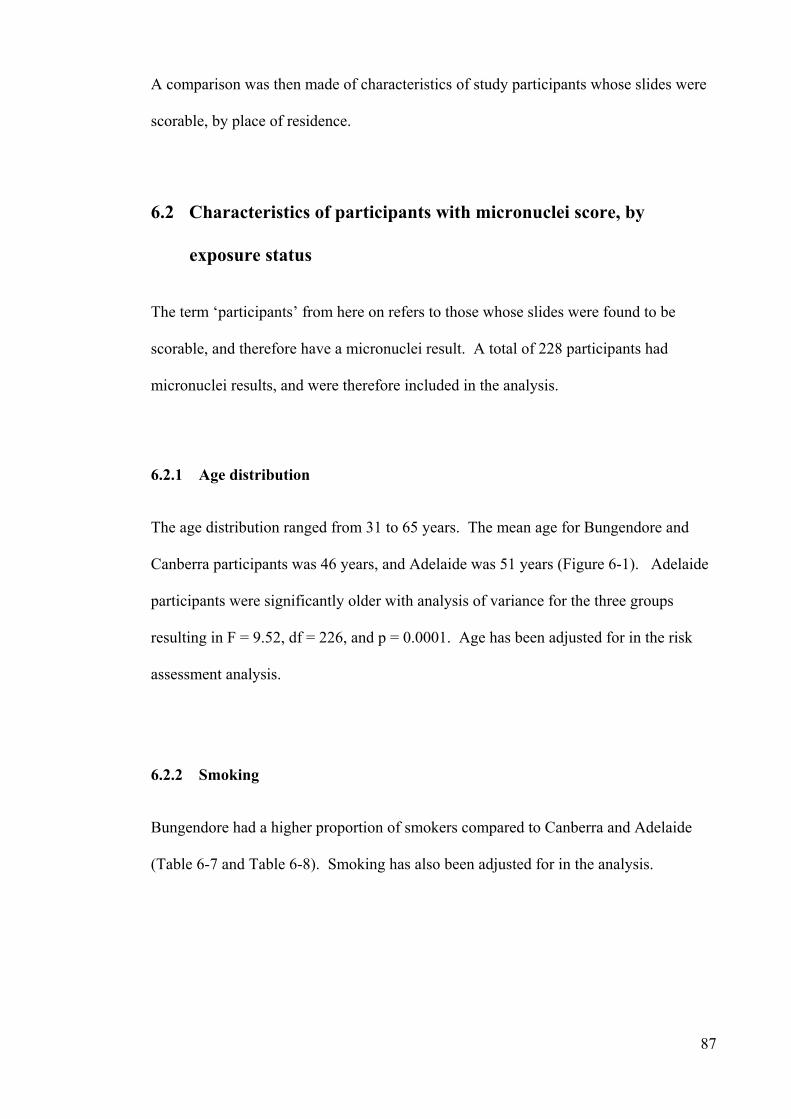
A comparison was then made of characteristics of study participants whose slides were

scorable, by place of residence.

6.2 Characteristics of participants with micronuclei score, by

exposure status

The term ‘participants’ from here on refers to those whose slides were found to be

scorable, and therefore have a micronuclei result. A total of 228 participants had

micronuclei results, and were therefore included in the analysis.

6.2.1 Age distribution

The age distribution ranged from 31 to 65 years. The mean age for Bungendore and

Canberra participants was 46 years, and Adelaide was 51 years (Figure 6-1). Adelaide

participants were significantly older with analysis of variance for the three groups

resulting in F = 9.52, df = 226, and p = 0.0001. Age has been adjusted for in the risk

assessment analysis.

6.2.2 Smoking

Bungendore had a higher proportion of smokers compared to Canberra and Adelaide

(Table 6-7 and Table 6-8). Smoking has also been adjusted for in the analysis.

87

Figure 6-1. Age (in quartiles) of participants by region of residence

Age

in y

ears

30

35

40

45

50

55

60

65

Bungendore (n=85) Canberra (n=85) Adelaide (n=58)

Table 6-7. Proportion of smokers by region of residence

Smoker (%) Non smoker (%) Total (%)

Bungendore 27 (32) 58 (68) 85 (100)

Canberra 13 (15) 72 (85) 85 (100)

Adelaide 13 (22) 45 (78) 58 (100)

Total 53 (23) 175 (77) 228 (100)

χ2 = 6.4921, df = 2, p = 0.04

88

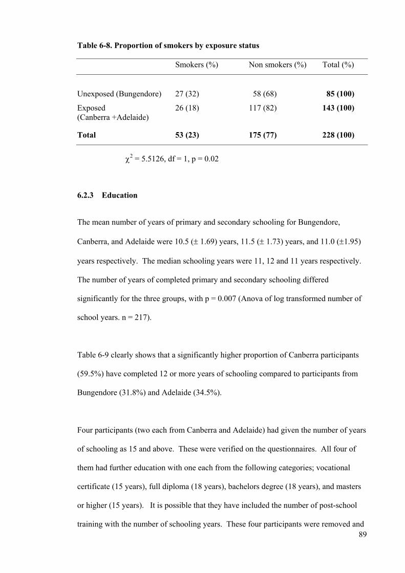
Table 6-8. Proportion of smokers by exposure status

Smokers (%) Non smokers (%) Total (%)

Unexposed (Bungendore) 27 (32) 58 (68) 85 (100)

Exposed 26 (18) 117 (82) 143 (100) (Canberra +Adelaide)

Total 53 (23) 175 (77) 228 (100)

χ2 = 5.5126, df = 1, p = 0.02

6.2.3 Education

The mean number of years of primary and secondary schooling for Bungendore,

Canberra, and Adelaide were 10.5 (± 1.69) years, 11.5 (± 1.73) years, and 11.0 (±1.95)

years respectively. The median schooling years were 11, 12 and 11 years respectively.

The number of years of completed primary and secondary schooling differed

significantly for the three groups, with p = 0.007 (Anova of log transformed number of

school years. n = 217).

Table 6-9 clearly shows that a significantly higher proportion of Canberra participants

(59.5%) have completed 12 or more years of schooling compared to participants from

Bungendore (31.8%) and Adelaide (34.5%).

89

Four participants (two each from Canberra and Adelaide) had given the number of years

of schooling as 15 and above. These were verified on the questionnaires. All four of

them had further education with one each from the following categories; vocational

certificate (15 years), full diploma (18 years), bachelors degree (18 years), and masters

or higher (15 years). It is possible that they have included the number of post-school

training with the number of schooling years. These four participants were removed and

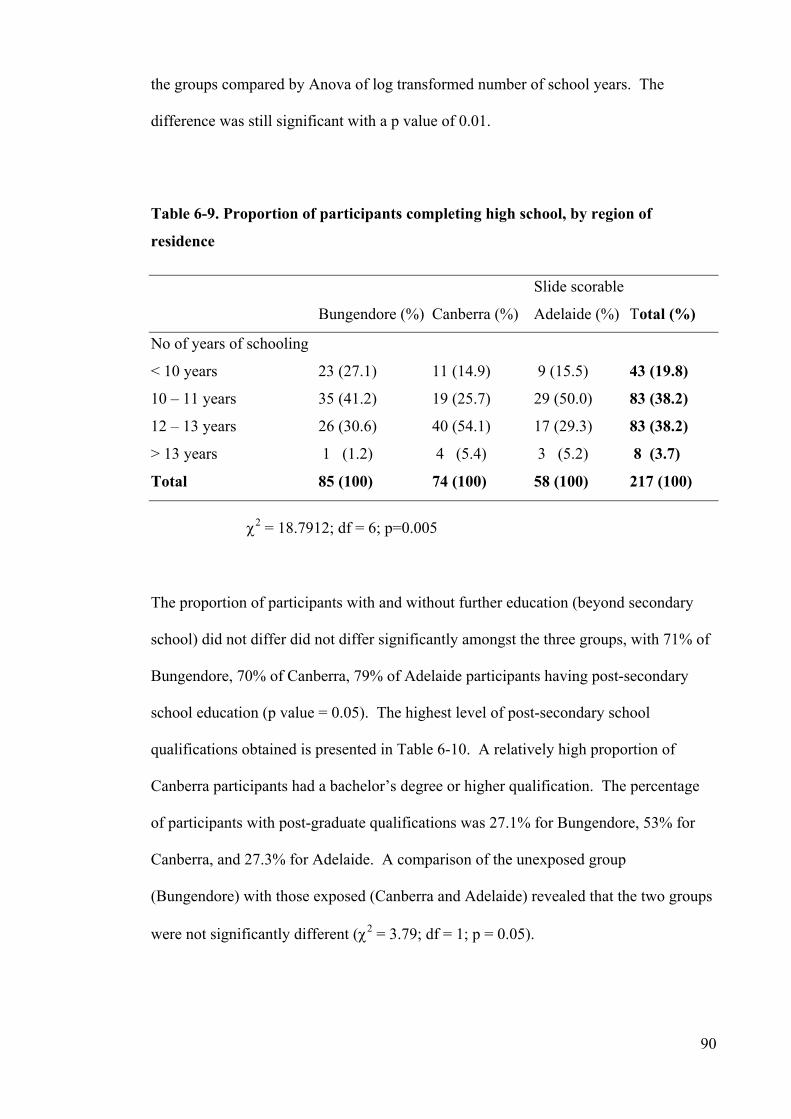
the groups compared by Anova of log transformed number of school years. The

difference was still significant with a p value of 0.01.

Table 6-9. Proportion of participants completing high school, by region of

residence

Slide scorable

Bungendore (%) Canberra (%) Adelaide (%) Total (%)

No of years of schooling

< 10 years 23 (27.1) 11 (14.9) 9 (15.5) 43 (19.8)

10 – 11 years 35 (41.2) 19 (25.7) 29 (50.0) 83 (38.2)

12 – 13 years 26 (30.6) 40 (54.1) 17 (29.3) 83 (38.2)

> 13 years 1 (1.2) 4 (5.4) 3 (5.2) 8 (3.7)

Total 85 (100) 74 (100) 58 (100) 217 (100)

χ2 = 18.7912; df = 6; p=0.005

The proportion of participants with and without further education (beyond secondary

school) did not differ did not differ significantly amongst the three groups, with 71% of

Bungendore, 70% of Canberra, 79% of Adelaide participants having post-secondary

school education (p value = 0.05). The highest level of post-secondary school

qualifications obtained is presented in Table 6-10. A relatively high proportion of

Canberra participants had a bachelor’s degree or higher qualification. The percentage

of participants with post-graduate qualifications was 27.1% for Bungendore, 53% for

Canberra, and 27.3% for Adelaide. A comparison of the unexposed group

(Bungendore) with those exposed (Canberra and Adelaide) revealed that the two groups

were not significantly different (χ2 = 3.79; df = 1; p = 0.05).

90

Table 6-10. Highest level of completed post-secondary school education obtained

by study participants, by region of residence

Highest education level

(post-secondary) Bungendore (%) Canberra (%) Adelaide (%) Total (%)

Vocational certificate 10 (16.9) 4 (8.2) 6 (13.6) 20 (13.2)

Trades certificate 25 (42.4) 13 (26.5) 18 (40.9) 56 (36.8)

Associate diploma 7 (11.9) 3 (6.1) 2 (4.6) 12 (7.9)

Full diploma 1 (1.7) 3 (6.1) 6 (13.6) 10 (6.6)

Bachelors’ degree 10 (16.9) 13 (26.5) 10 (22.7) 33 (21.7)

Graduate diploma 5 (8.5) 8 (16.3) 1 (2.3) 14 (9.2)

Masters degree or higher 1 (1.7) 5 (10.2) 1 (2.3) 7 (4.6)

Total 59 (100) 49 (100) 44 (100) 152 (100)

6.2.4 Beverage consumption

Patterns of beverage consumption were also compared among the three study groups.

Table 6-11 below presents the number, and proportions from each study community,

reporting consumption of the various beverages. The table shows that Adelaide

residents consumed less tap water at both the work place and at home. Bungendore and

Adelaide residents consumed more bottled water compared to Canberra residents.

Bungendore and Canberra residents consumed more alcohol than did Adelaide

residents. Adelaide water, although meeting both WHO and Australian Drinking water

guidelines, is of lower aesthetic quality compared to either Canberra or Bungendore. It

is therefore not surprising that Adelaide residents consume more bottled water.

91

Table 6-11. Fluid consumption by study participants during two-week study

period, by region of residence

Number (%) reporting intake

Bungendore n = 85

Canberra n = 85

Adelaide n = 58

χ2 (df) p value

Tap water*

Work water**

Bottled water

Coffee

Hot beverages

(incl. Coffee)

Alcohol

61 (72)

32 (38)

18 (21)

78 (92)

82 (96)

75 (88)

71 (84)

32 (38)

13 (15)

73 (86)

83 (98)

76 (89)

34 (59)

10 (17)

19 (33)

49 (84)

55 (95)

44 (76)

10.9 (2)

8.21 (2)

6.19 (2)

2.12 (2)

5.92 (2)

0.004

0.02

0.046

0.35

1.00***

0.05

*Tap water = tap water from the community water supply at place of residence

**Work water = water from the community water supply at work place

***Fisher’s exact test for combined Canberra / Adelaide (exposed) vs Bungendore (unexposed)

6.3 Exposure levels

Exposure levels for the three regions have been presented as available dose

(concentration of THM and absorbable organic halogen (AOX) in reticulated water),

intake dose (adjusted for individual variation in exposure), and internal dose (THM

concentrations in urine). In the following box plots created in STATA version 6, the

dots outside the box plot are outliers, defined by STATA program to be readings > 1.5

times the inter quartile range.

92

6.3.1 Available dose (concentration in reticulated water)

The unchlorinated Bungendore water contained no detectable levels of THMs. In

Canberra and Adelaide, total THM in reticulated water ranged from 37.75 – 157.25 µg/l

(mean = 88.20, std deviation = 39.73, median = 64.25). The distributions differed

significantly in the two regions (figure 6-2) with Adelaide having significantly higher

levels compared with Canberra (Mann-Whitney test: Canberra vs Adelaide: z = -10.145,

p <0.0001).

Figure 6-2. Distribution of available dose of total THM, by region of residence

Tota

l TH

M c

once

ntra

tion

in m

icro

gram

s/lit

re

0

40

80

120

160

Bungendore (n=85) Canberra (n=85)Adelaide (n=58)

The four THM compounds, when examined separately, showed that chloroform (the

principle chlorinated compound) occurred predominantly in Canberra water, while

bromoform and the mixed haloforms were found in Adelaide water (Figure 6-3 and 6-

4). The relatively higher proportion of brominated compounds in reticulated water in

Adelaide (as seen in figure 6-4) was also shown by Simpson et al in a comparison of

drinking water of Adelaide and Newcastle in NSW. The predominance of brominated

THMs in Adelaide has been attributed to the higher salinity, and occurrence of natural

93

bromide ion which reacts with the relatively higher concentration of naturally occurring

organic matter [6].

To compare the relative proportions of THM compounds in Canberra and Adelaide

reticulated water, the mean total THM concentration has been proportionately

represented in figure 6-4 such that the area of the chart represents the magnitude of

(mean) total THM in the water. The square root of the mean THM concentration was

obtained, and the graphs proportioned accordingly. Bungendore has not been included

in the comparison, as THMs were not detected in Bungendore water.

94

Figure 6-3. Distribution of available dose of THMs, by compound and region of

residence

Chloroform p value Mann Whitney test) itr

e 80

ram

s/ l

<0.0001 mic

rC

once

ntra

tion

inog

0

20

40

60

Bungendore (n= 85) Canberra (n = 85) Adelaide (n = 58)

Bromodichloromethane

0.0001

ogra 60

atio

n i

40

Con

cent

rn

mic

rm

s/ li

tre

0

20

80


Dibromochloromethane

ms/

litr

<0.0001

mic

rC

once

ntra

tion

inog

rae

0

20

40

60

80


Bromoform

0.0001

ogra

m

once

ntr

20

Cat

ion

in m

icr

s/ li

tre

0

40

60

80


95

Figure 6-4. Proportionate representation of mean total THM concentrations in Canberra and Adelaide reticulated water (Available dose)

Canberra – Mean total THM = 57.74

Canberra

Dibromochloro-methane 37.9%

Bromoform 9.8%

Adelaide – Mean total THM = 133.09

Bromodichloro-methane 2.2%

µg/l

Chloroform 97.8%


Chloroform 19.8%

µg/l

96

AOX levels in Canberra ranged from 140 – 265 µg/l, with mean and standard deviations

being 219.29 µg/l and 33.78 µg / l respectively (n=85). In Adelaide, AOX

concentrations ranged from 220 – 425 µg/l with mean and standard deviations of 327.33

µg/l and 59.18 µg/l respectively (n=58). These concentrations differed significantly

with t = -13.8558; p<0.0001. Bungendore was not included in the comparison as no

AOX was detected in Bungendore water. AOX distributions have been graphically

represented in Figure 6-5.

Figure 6-5. Mean AOX concentration in quartiles for reticulated water, by region

of residence

00

100

200

300

400

500


Con

cent

ratio

n in

µg/

litre

6.3.2 Intake dose (available dose adjusted for individual beverage consumption)

The following section describes intake dose for study participants, as estimated by fluid

intake diary records and by a retrospective questionnaire. All intake dose distributions

showed extreme negative skewness. Intake dose of total THM from the fluid intake

diary was nil for all Bungendore participants (since the water contained no DBPs) while

the estimates for Canberra and Adelaide ranged from 2.9 to 469.5 µg/kg -day (mean =

97

139.9 µg/kg - day, std deviation = 95.6 µg/kg-day, and median = 117.6 µg/kg-day). The

estimate using retrospective questionnaire ranged from 0 to 409.4 µg/kg-day, (mean =

35.4 µg/kg-day, std deviation = 82.8 µg/kg-day, and median = 20.0 µg/kg-day). Figure

6-6 presents the distributions in quartiles for the three study communities. The Mann

Whitney test comparing Canberra and Adelaide showed that the distributions of the

individual THM compounds differed significantly between the two communities (by

both estimates), with all p values being <0.0001. Adelaide water contained a

significantly higher proportion of brominated compounds. This is due to the trace

amounts of bromide ions in Adelaide raw water supply and preferential formation of the

bromide by-products. Intake dose of total THMs, when estimated by fluid intake diary

records, differed significantly between the two groups, with Adelaide having

significantly higher levels (p = 0.03). The estimate by of total THM intake by

retrospective questionnaire however, did not differ significantly (p=0.2).

Chapter seven provides a comparison of fluid intake estimates made by fluid intake

diary and questionnaire. Although the two estimates did not differ greatly, wherever

intake dose was used in a regression analysis (chapter eight), the analysis was

undertaken using both estimates of intake dose (i.e. by fluid intake diary and

questionnaire).

98

Figure 6-6. Distributions of intake dose of THM as estimated by fluid intake diary

and retrospective questionnaire, for the three study communities

Fluid intake diary Retrospective questionnaire

Chloroform

0B ) C


50

100

150

200

250

300

350

ungendore (n=85 anberra (n=85) Adelaide (n=58)0

50

100

150

200

250

300

350

400


Inta

ke d

ose

in m

icro

gram

s/kg

-day

0

50

100

150


Inta

ke d

ose

in m

icro

gram

s/kg

-day

0

50

100

150


Con

cent

ratio

nin

mic

rogr

ams/

liter

Inta

ke d

ose

in m

icro

gram

s/kg

-day

Inta

ke d

ose

in m

icro

gram

s/kg

-day

Cont’d

99

Figure 6-6. Cont’d. Distributions of intake dose of THM as estimated by fluid

intake diary and retrospective questionnaire, for the three study communities


100100

Inta

ke d

ose

in m

icro

gram

s/kg

-day

Bromoform

Total THM

0

25

50

Bungendore (n=85) Canberra (n=85) Adelaide (n=58)0

25

50


0

100

200

300

400

500

Bungendore (n=85) Canberra (n=85) Adelaide (n=58)0

100

200

300

400

500


Inta

ke d

ose

in m

icro

gram

s/kg

-day

Inta

ke d

ose

in m

icro

gram

s/kg

-day

0

50

150

200

Bungendore (n=85) Canberra (n=85) Adelaide (n=58) 0

50

150

200


Inta

ke d

ose

in m

icro

gram

s/kg

-day

Inta

ke d

ose

in m

icro

gram

s/kg

-day

Inta

ke d

ose

in m

icro

gram

s/kg

-day

100

6.3.1 Internal dose (concentrations in urine)

Internal dose for Canberra and Adelaide were also distributed with negative skewness.

Total THM concentrations in Canberra ranged from 0 to 6.82 µg/l (mean = 0.67 µg/l,

std deviation = 1.17 µg/l, median = 0.33 µg/l), while Adelaide had levels ranging from

0.1 to 3.14 µg/l (mean = 0.60 µg/l, std deviation = 0.51 µg/l, median = 0.48 µg/l). As

expected, no THMs were detected in urine of Bungendore participants. This

demonstrated that the Bungendore participants (i.e. the unexposed group) were not

exposed to THMs from other sources. The distributions of internal dose are compared in

Figure 6-7 and show numerous outliers defined by Stata to be readings > 1.5 times the

inter quartile range.

The Mann Whitney test was employed to effect a meaningful comparison of exposure

of Canberra and Adelaide trial participants (figure 6-7). Overall exposure to THMs was

highest in Adelaide. Adelaide has highly modified local water supply catchments and

also relies on Murray River water pumped from Mannum. Natural organic matter levels

are relatively high and, while strenuous efforts have been made to avoid DBP formation

in recent years, THM levels are still relatively high by international standards. Since

Adelaide water is slightly brackish and contains small amounts of bromide ion, the

proportion of brominated DBPs and THMs is higher in Adelaide than in Canberra

water.

Overall, however, the amounts of bromoform are similar in both Adelaide and Canberra

water. The amount of chloroform in Canberra water is actually higher than for

Adelaide, but when the mixed bromochloro-THMs are taken into account, the total

exposure of Adelaide participants to THMs (and to AOX) is actually much higher.

101

Figure 6-7. Distribution of internal dose of THM concentrations (in quartiles), by

compound and region of residence

Chloroform Mann Whitney test

p = 0.0001

og

ram

sco

ncen

tratio

n in

mic

r/li

tre

0

.5

1

1.5

2



p <0.0001

ogra

ms

e

2

conc

entra

tion

in m

icr

/litr

0

1



p <0.0001

gra 4

conc

entra

tion

in m

icro

ms/

litre

0

2

6


Bromoform 6

p = 0.08 tre

rogr

a 4

conc

entra

tion

in m

icm

s/li

0

2


102

Figure 6-7 cont’d. Distribution of internal dose of THM concentration (in

quartiles), by region of residence

Mann Whitney test t p = 0.01 8

conc

entra

tion

in m

icro

gram

s/lit

re

0

2

4

6

otal THM


Internal dose for total THM has been proportioned graphically in figure 6-8. It depicts

the abundance of the individual compounds. In comparison to available dose of total

THM shown in figure 6-4 where only chloroform and bromodichloromethane were

detected in Canberra water, in urine, bromine compounds accounted for over 70% of the

total THM components. There are several possible reasons for this difference in THM

components in water and urine. A likely explanation is that the assay used for THMs in

urine had a lower detection level (of 0.01 µg/l) compared to the assay used for water

(0.1 µg/l). It is therefore possible that the bromine compounds may have been present

in low concentrations in the water, but not at levels sufficient to be detected with the 0.1

µg/l threshold level. This does not however explain the difference in the proportions of

the various compounds in water and urine and is therefore an unlikely proposition.

Bromoform is used in food processing, and is a potential – if not a highly probable -

source of exposure to this compound. Chloroform, which is highly volatile can be

easily lost by evaporation, or by being metabolised.

103

In the presence of bromine, even at vanishingly low concentrations, brominated DBPs

are formed in water from organic matter - in the presence of hypochlorous acid - in

preference to chlorinated byproducts. To explain the higher proportion of bromine

compounds in urine, it is necessary to assume that either the more volatile fractions

(mainly chloroform) are selectively removed and expired or that selective

biodegradation of chloroform and C-Cl bonds of mixed trihalomethanes occurs in vivo.

A much less likely proposition is that carbon-chlorine bonds are replaced by bromine in

vivo and that the water source makes a critical contribution to body bromide levels.

What is also clear from comparing available and internal doses of total THM is that,

with available dose, Adelaide had a higher mean total THM level compared to

Canberra, whereas with internal dose, mean total THM was higher in Canberra. This is

possibly explained by the differences in true exposure between the two communities.

Even though the reticulated water in Adelaide had higher concentrations of THMs, tap

water intake in Adelaide was shown to be lower in Adelaide when compared with

Canberra (table 6-10). It was noted from interviews (although this information was not

formally collected) that many Adelaide residents used rainwater tanks for domestic use

including showering. Exposure is also determined by dermal and inhalation exposure.

Combining the lower tap water intake and possible use of other sources of water for

domestic use, it is highly likely that Adelaide participants are exposed to less THMs

than the Canberra participants are. This would result in lower concentrations of THMs

in the body, resulting in lower internal dose. This further highlights the importance of

individual exposure assessment and the benefits if using a biological marker rather than

estimating exposure from interview data.

104

Figure 6.8. Proportionate representation of mean total THM concentrations in urine of Canberra and Adelaide participants (internal dose)

Chloroform 13.8%

Bromoform 61.3%

Canberra – Mean total THM = 0.80 µg/l

Bromodichloromethane13.8%

Dibromochloromethane 11.3%

Dibromochloro-methane 7.7%


Bromoform 41.5%

Chloroform 18.5%

Adelaide – Mean total THM = 0.64 µg/l

105

6.4 Outcome – Micronuclei frequency

The prevalence of micronuclei in bladder epithelial cells has been summarised by

region, in table 6-12. The total number of cells scored for Bungendore, Canberra and

Adelaide were 127 431, 74 585, and 52 781 respectively. The average numbers of cells

scored per participant for the three regions were 929, 496, and 430 respectively.

Although it was intended to score a minimum of 1000 cells per participant, the density

of cells on slides did now enable as large numbers as that to be scored per participant.

Table 6-12. Unadjusted prevalence of micronuclei in bladder epithelial cells, by

region

Cells % abnormal micronuclei per 1000 Counted* cells normal cells

range mean median

Bungendore (n=85) 127,431 34.0 0 to 22.7 1.7 0.9

Canberra (n=85) 74,585 32.9 0 to 11.4 1.0 0.4

Adelaide (n=58) 52,781 37.1 0 to 20.4 1.7 0.1

* Cells counted = normal and degenerated / abnormal cells

The proportion of abnormal cells did not differ significantly between the three regions,

with 32.9 to 37.1% of cells being abnormal. A chi-square test was performed to

compare the expected proportions: this resulted in p=0.78 (χ2 = 0.50; df=2).

Flow cytometry data have been described in chapter nine.

106

6.5 Association between exposure and outcome

Scatter plots examining associations between the exposure indices and prevalence of

micronuclei did not show an obvious linear or non-linear association (appendices 1 to

3a). Detailed assessment of the association using regression models, is presented in

chapters 8 and 9.

6.6 Association of potentially confounding variables with exposure

and outcome

The potentially confounding variables were examined for associations with the exposure

indices (appendices 4 to 7). The variables were not correlated with the highest

correlation coefficient being 0.40 between available dose of chloroform and serum

folate levels (appendix 4).

Potentially confounding variables were also examined for associations with the

frequency of micronuclei (appendix 8). Lifetime history of working with paint, and

lifetime history of working with leather as part of a hobby were the only two variables

that were significantly associated with the outcome measure. Of these, the former

association was protective (rr=0.61, 95% CI 0.41 to 0.92). This is likely to be a chance

occurrence more than a true estimate of effect.

The variables considered as potential confounders in this study are factors that are

known to be risk factors for bladder cancer and / or known to effect cell integrity. The

confounding role of these variables has been assessed further in chapter eight by

examining the effect of introducing these variables in to the regression analysis.

107

6.7 Bladder cancer incidence in the three study communities

Prior to examining the association between exposure to THM and frequency of

micronuclei at an individual level for study participants, the rates for bladder cancer (for

which micronuclei is being used as an early pre-clinical marker) for the three study

communities was examined. Bungendore is situated within the Local Government Area

(LGA) of Yarrowlumla. This LGA mainly consist of rural villages where community

water supplies are not chlorinated.

Table 6-13. Bladder cancer incidence rates for the study communities

Males Females n ASR1 ASR2 n ASR1 ASR2 (Australia 1991) (World) (Australia 1991) (World)

Yarrowlumla NSW 1991-953 2 - 10.9 0 - 0 ACT 1985-894 11 - 11.6 4 - 2.9 ACT 1991-955 12 15.6 4 - 4.3 ACT 1992-966 15 17.6 - 4 3.7 - ACT 1993-977 15 17.2 - 5 4.1 - SA 1985-894 119 - 12.5 41 - 3.2 SA 1991 –955 122 17.0 41 - 4.2 SA 1992-966 124 17.0 - 40 4.0 - SA 1993-977 125 16.7 - 43 4.2 - Australia 85-894 1609 - 15.2 563 - 4.3 Australia 91-955 1976 23.7 15.9 646 6.1 4.2

Australia 93-977 1986 22.6 15.1 695 6.2 4.2 1 Age standardised incidence rates using Australian Population Standard, per 100,000 population 2 Age standardised incidence rates using World Population Standard, per 100,000 population 3 Source: [91] 4 Source: [92] 5 Source: [93] 6 Source: [94] 7 Source: [46] 108

Comparable incidence rates were available for the years 1991 to 1995, although

incidence rates adjusted for World Standards were not available for ACT and SA. By

examining available information, it may appear that the ASR (adjusted for World

Standards) show a trend with increasing rates going from Yarrowlumla LGA, to ACT,

and SA. This may very well suggest a correlation between chlorination and bladder

cancer incidence rates. This picture is however not so clear when examining subsequent

incidence rates for 1991-95, 1992-96 and 1993-97, which have been adjusted for the

Australian Standard 1991. Here, ACT and SA have similar incidence rates, which are

lower than the overall Australian rates. The higher Australian rate is due to the high

incidence rates in VIC, QLD and TAS, where incidence rates are in the high 20’s [93],

[94], [46]. Without knowing the chlorination and DBP levels in these States, it is not

possible to know whether this information supports the association between chlorination

and bladder cancer.

An ecological comparison such as this does not take into account other factors that may

be contributing to the observation of bladder cancer incidence rates. The prevalence of

other risk factors to bladder cancer (such as cigarette smoking, use of pesticides or

chemicals) may differ between these communities and may be contributing to the

observed differences in bladder cancer incidence.

Such an ecological comparison can however suggest an association between the two

factors (chlorination level and bladder cancer), and would justify further investigation of

this association.

109

Chapter 7. Estimation of fluid intake by diary records

and by retrospective questionnaire

The study presented in this dissertation builds on previous studies by assessing exposure

at an individual level. In order to estimate individual exposure to disinfection by-

products (DBP) from drinking chlorinated water, participants were asked to report fluid

intake over a two-week study period. This was achieved using two methods, a fluid

intake diary and a retrospective interviewer administered questionnaire.

7.1 Aim

The aim of this component of the study was to assess the level of agreement between

two methods for estimating fluid intake, using fluid intake diary records and using a

retrospective interviewer administered questionnaire. Comparisons were made for tap

water, water based hot beverages (coffee and tea), and for alcohol intake.

7.2 Methods

The study period was of two-week duration. During which time, participants were

asked to keep a record of all beverages consumed. A fluid intake diary was provided

for this purpose. At the end of the two-week period, a questionnaire was administered

by telephone to recall fluid intake for the duration of the study period.

110

7.2.1 The diary

The diary was based on a format presented by Armstrong et al, and modified to suit the

purpose of this study [95, page 210]. A member of the research team met with the

participants individually and explained the procedure. Participants were instructed to

record fluid intake at least on a daily basis. Information to be recorded on the page per

day diary included date, time, type of drink, amount (using a code), number of serves,

and place (Appendix 26). Time was included to aid participants to recall fluid intake

over the day, especially if they were recording on a daily basis instead of on an ongoing

basis. For the ‘amount’ pre-coded categories were provided. e.g. cup, mug, small glass,

medium glass etc. Space was allocated to place where beverage consumed. This

information was to determine the chlorination status of the water consumed.

Intake volume for the two weeks was computed by converting the amount or portion

size in to milliliters (ml) and summing intake by beverage type. This was then

converted to average daily intake.

7.2.2 The questionnaire

At the end of the two-week period, a member of the research team telephoned the

participant and administered a questionnaire to independently determine fluid intake

over the study period, without referring to the diary. The participants were asked to

recall what he or she had to drink over the preceding two weeks, without reference to

diary records. The questions were worded as follows:

Have you drunk tap water in the last two-weeks?

If No, the interviewer would go on to the next beverage. If Yes:

Was it every day, every week, or less often?

111

If the participant had responded every day, he was asked:

On average, how many drinks would you have had a day?

Or if every week:

On average, how many drinks would you have had per week?

Or if less often:

How many drinks in total would you have had in the last two weeks?

This was followed up by:

What size portion did you usually have? Was it a cup, mug, small, medium, or

large glass, half bottle, small or large bottle?

Intake volume over the two-weeks was calculated for each beverage using the following

formula:

{(portions per day x portion size in ml) x 14} + {(portions per week x portion

size in ml) x 2} + one-off intake in ml

Average daily intake was computed from this information.

With both methods, conversion of amount or portion size to volume consumed was

done using the following conversion rates.

Cup = 250 ml Half bottle/stubbie/normal can = 375 ml

Mug = 300 ml Standard bottle = 750 ml

Small glass/pony = 100 ml Half nip = 15 ml

Medium glass/middy = 284 ml Nip = 30 ml

Large glass/schooner = 425 ml Double nip = 60 ml

Small bottle/can = 285 ml Other = as specified

Beverages were grouped in to broad categories. The main groups of interest were tap

water, water based hot beverages (coffee and tea), and alcohol. With each beverage, if

no intake were reported, it was assumed that there was no intake of that beverage during

the study period, and therefore entered in the database as zero intake.

112

7.2.3 Comparison of fluid intake estimates

Diaries and questionnaires that had been incompletely filled were not used for the

comparison. Statistical comparison of the two methods was undertaken using two

techniques. The first technique utilised a method recommended by Bland and Altman

for method comparison studies [96], [97, chapter14.2]. The two variables were plotted

against each other, followed by plotting the average readings against the difference at an

individual level. This provides a graphical estimate of the differences.

The second technique for comparing fluid intake estimates made by the two methods

was the kappa test. Water intake was categorised in quintiles, and the level of

agreement between categories was examined by weighted kappa test. When dividing in

to quintiles, if zero intake was the 20th centile, zero was categorised as the first category,

and the rest were equally divided in to four groups. Kappa was used because it is a

quantitative method of assessing level of consistency between two methods used on the

same subject, whether it be by two observers, on two occasions, or using two

procedures. Kappa is the usual test to assess agreement in dietary records. Weighted

kappa is used here giving different weights to the magnitude of difference. For

example, in using weighted kappa, a difference of one category is considered to be less

of a discrepancy than a difference of two or three categories.

7.2.4 Test-retest reliability of questionnaire

The ability for an instrument to reproduce results when used at a different time (i.e.

reliability of questionnaire) was tested for in Bungendore only for logistic reasons.

113

Administering the questionnaire a fortnight after administering the initial retrospective

questionnaire tested repeatability. The period of recall was the preceding two-weeks,

i.e. the two weeks since administering the last questionnaire. Due to the demand on

respondent time, repeatability of fluid intake diary was not conducted.

7.3 Results

A total of 281 participants had complete records for diary and questionnaire. These

records were used in the comparison presented here. All participants were males due to

a selection criterion set for the main study, and they were aged between 30 and 65 years

(section 5.3).

7.3.1 Fluid intake

According to the fluid intake diary, 81.9% of participants drank tap water, 97.5% drank

hot beverages, and 92.5% drank alcohol during the study period. The retrospective

questionnaire identified a lower intake of tap water (70%) and alcohol (83.3%) intake in

terms of both proportion consuming and amount consumed (Table 7-1). Hot beverage

consumption did not differ greatly except for a small increase in the amount estimated

by questionnaire.

7.3.2 Bland and Altman Method

Plotting of fluid intake by diary records versus questionnaire (figure 7-1) indicate that

there is a linear relationship between the two variables. As with most of such data, there

is clustering of points at the base making it difficult to assess the differences.

114

Table 7-1. Beverage consumption pattern during the study period, as estimated by diary records and by questionnaire

Daily Intake in ml (rounded to the nearest 100 ml)

Diary (n=281) Questionnaire (n=281)

Beverage type

Number reporting beverage

consumption (%)

Range Median Number reportingbeverage

consumption (%)

Range Median

Tap water 230 (81.9) 100 – 5200 300 191 (70.0) 100 - 4400 100

Hot beverages 274 (97.5) 100 – 3400 1000 272 (96.8) 100 - 3900 1100

Alcohol 260 (92.5) 100 – 4400 400 234 (83.3) 100 - 3300 200

115

Figure 7-1. Scatter plots of diary versus questionnaire intake estimates

Spearman rank correlation

Tap water r = 0.74 5.

Dia

ry e

stim

ate

in

l/day

questionnaire estimate - in l/day0 2.2 4.4

0

2.6

2

Hot beverages r = 0.84 2.

Dia

ry e

stim

ate

- in

l/day

questionnaire estimate - in l/day0 1.25 2.5

0

1.05

1

Alcohol r= 0.76 2.

Dia

ry e

stim

ate

- in

l/day

questionnaire estimate - in l/day1.0

0 2.00

6

1.3

116

Plotting of differences between the two variables (diary – questionnaire) showed the

scatter of difference increasing as the average of the two measures increase, i.e. the

difference is proportional to the mean (figure 7-2). The recommendation for this

situation by Bland and Altman is to plot log transformed data. However, the authors

also mention that due to the complexity of interpreting back transformed data, only log

transformation is recommended for this technique. The fluid intake data contains many

zeros, and log transformation requires further manipulation. The back transformation

results in negative numbers, which as indicated by Bland and Altman, are difficult to

interpret. Therefore, in spite of large standard deviations obtained, raw data are used to

examine any difference.

Figure 7-2 also includes the 95% confidence intervals demonstrating the limits of

agreement. With tap water, the mean difference (diary – questionnaire) was 13.6

ml/day. Based on these data, questionnaire intake of tap water could under estimate or

exceed diary intake by about 1200 ml/day. Similarly, the mean difference in hot

beverage intake was not big at 169 ml/day, but the difference could be anything from

about -1000 to 700 millilitres. A similar difference was observed with alcohol intake.

These differences are not huge, but the impact would depend on the purpose of the

comparison.

117

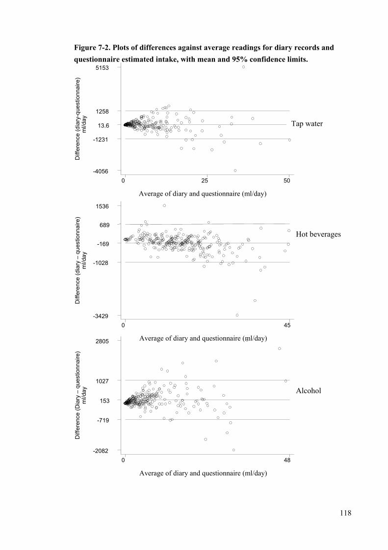
Figure 7-2. Plots of differences against average readings for diary records and questionnaire estimated intake, with mean and 95% confidence limits.

1258

s

Diff

eren

ce (d

iary

-que

stio

nnai

re)

ml/d

ay

Average of diary and questionnaire (ml/day)

0 25 50-4056

-1231

13.6

5153D

iffer

ence

(dia

ry –

que

stio

nnai

re)

ml/d

ay


0 45-3429

-1028

-169

689

1536

Diff

eren

ce (D

iary

– q

uest

ionn

aire

)m

l/day


0 48-2082

-719

153

1027

2805

Hot beverage
Alcohol
Tap water

118

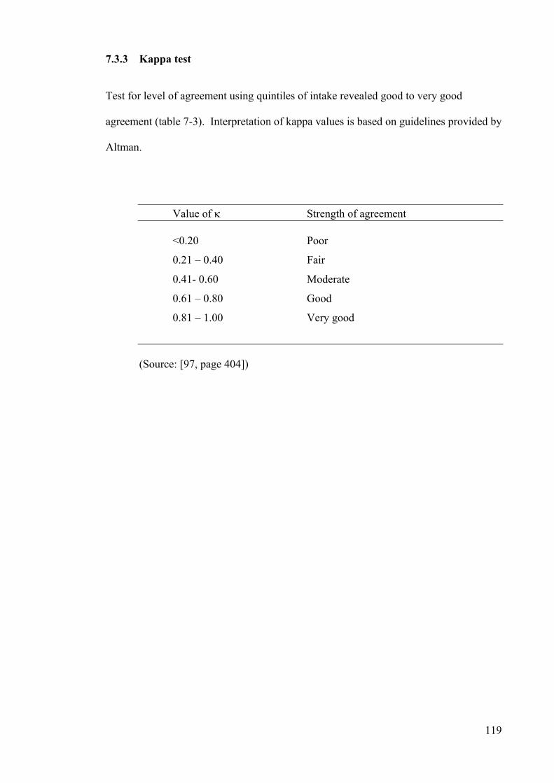
7.3.3 Kappa test

Test for level of agreement using quintiles of intake revealed good to very good

agreement (table 7-3). Interpretation of kappa values is based on guidelines provided by

Altman.

Value of κ Strength of agreement <0.20 Poor

0.21 – 0.40 Fair

0.41- 0.60 Moderate

0.61 – 0.80 Good

0.81 – 1.00 Very good

(Source: [97, page 404])

119

Table 7-2. Level of agreement between fluid intake diary and questionnaire

Quintiles

1 2 3 4 5 Total Weighted

Kappa (95% CI)

Tap water

1 53 1 0 1 0 55

2 18 22 13 3 1 57

3 9 15 18 11 4 57 0.68

4 6 4 10 23 13 56 (0.57 to 0.80)

5 4 6 5 12 29 56

Total 90* 48 46 50 47 281

Hot beverage

1 42 11 1 0 1 55

2 13 28 14 1 0 56

3 0 14 28 12 4 58 0.84

4 0 3 13 27 13 56 (0.72 to 0.96)

5 1 0 1 16 38 56

Total 56 56 57 56 56 281

Alcohol

1 34 16 4 1 0 55

2 13 24 17 3 0 57

3 5 12 19 19 2 57 0.78

4 1 4 13 27 11 56 (0.66 to 0.90)

5 1 2 3 7 43 56

Total 54 58 56 57 56 281

*All zero intake

120

7.3.4 Test-rest reliability

Of the original 147 participants from Bungendore, 139 completed the retrospective fluid

intake questionnaire two-weeks after completing the initial questionnaire. Short-term

repeatability of the retrospective questionnaire (after two-weeks) was found to be

moderate with Spearman’s correlation coefficients and kappa values for the three

beverage groups ranging from 0.51 to 0.56 (Table 7-3).

Table 7-3. Repeatability of the retrospective fluid intake questionnaire

Beverage

Spearman’s correlation

coefficient

Kappa value (95% CI)

Tap water Hot beverages Alcohol

0.55

0.51

0.56

0.55 (.039 to 0.72)

0.51 (0.35 to 0.67)

0.56 (0.40 to 0.72)

7.4 Discussion

Data from this study show that for the study population, the two methods had good

levels of agreement when estimating fluid intake over the two-week study period. This

finding is in keeping with Shimokura et al’s comparison of water intake by

questionnaire and a three day water diary, where Spearman’s correlation coefficient was

reported to be 0.75 [98]. Kappa values were not reported in this study. A similar study

conducted by the Cooperative Research Centre for Water Quality and Treatment also

found moderate to good level of agreement between a questionnaire and three-day water

intake diary, with weighted kappa for three age groups ranging from 0.57 to 0.74

(Personal communication from paper in preparation - [99]).

121

A comparison of alcohol intake estimates by quantitative food frequency questionnaire

and food diary reported Pearson’s correlation coefficients varying from 0.68 to 0.79 for

all respondents [100]. Un-weighted kappa statistics reported for the same study were

fair to moderate. It is possible that had weighted kappa statistics been estimated, the

level of agreement may have been higher. In general, use of food frequency

questionnaires to estimate alcohol intake has been found to compare well with other

methods, particularly weighed food records (WFR), as summarised by Smith et al

[101]. The authors summarise several studies with Pearson’s correlation coefficient for

alcohol ranging from 0.74 to 0.90. Their study reported energy adjusted Spearman’s

correlation coefficient of 0.66 for alcohol (comparing self-administered food frequency

questionnaire and WFR). Findings from the study presented here are consistent with

these previous reports.

The general picture obtained from this study shows that with tap water and alcohol, the

retrospective questionnaire estimates were higher than the diary estimates, whereas with

hot beverages, the diary estimate marginally exceeded the retrospective questionnaire

estimate. It is not possible to know for certain the reason for this pattern. If we assume

that the diary provides a more accurate estimate of intake, we could speculate that

intake of beverages such as water and alcohol that are likely to be influenced by

weather, social gatherings, and physical activity, can be overestimated by questionnaires

because of generalising behaviour. In contrast, hot beverage intake maybe more

routine, therefore its intake could be more accurately estimated by even generalising

behaviour.

122

Browsing of diaries and questionnaires obtained in this study revealed that discrepancy

appeared to be more of a problem when a particular beverage was not a regular intake,

although there was the occasional participant who had recorded regular intake in one

method but not in the other. Another common finding was that there was a general

tendency for one method to underestimate or overestimate intake compared to the other

method. That is, there was no haphazard variation in estimating fluid intake for a

particular beverage type.

The inconsistencies in obtaining information using the two methods may have

contributed towards the differences in fluid intake estimates observed. When the

retrospective questionnaire was administered by an interviewer, beverage types were

specified (e.g. tap water from community, tap water from work place, bottled water,

tank water, tea, brewed coffee, instant coffee, decaffeinated coffee, beer, wine, fortified

wine, and spirits). In the fluid intake diary, beverage type was left open, which may

have resulted in certain omissions. This is likely to have contributed to some of the

discrepancy in the estimates obtained from the two methods.

There are advantages and disadvantages associated with the use of diaries and

retrospective questionnaires in quantifying food or fluid intake. The main advantage of

using diaries is not requiring participants to summarise patterns of behaviour, whereas

questionnaires ask for usual behaviour. This is important for estimating intake of

beverages that may differ from day to day depending on person’s activities, weather etc.

Summarising may result in loss of information. For this reason, diaries are assumed to

have a high level of accuracy, especially in measuring current behaviour, because they

do not rely on memory.

123

However, they are associated with a large respondent burden, which may have been

responsible for only 81.4% (n=281) of the total 345 participants completing the diary

without leaving any pages blank. A review of response rates of studies using diaries

found the response rate to be generally between 50 – 96%. This is quite a wide range.

Feedback received in general from this study indicates that time was the main hindrance

to maintaining the diary.

Participation rates in studies utilising diaries have been found to be lower for those with

less than high school education, lower socio-economic class, elderly, and those who

have recently experienced stressful life events [95, page 213]. Diaries are also

associated with sources of error unless they are carefully prepared and participants

provided with proper instructions. They may require certain skills from participants.

Training of participants in recording and measuring is time consuming both to the

participant and research team. As a result, recruiting a representative sample may be

difficult. In the study presented here, each participant was visited individually and the

study procedure (including completing diary) was explained. These visits varied in

duration lasting from 15 minutes to up to an hour in a few cases. Instructions on

completing the diary took up a large proportion of this time. In addition, a toll-free

telephone number was provided for participants to call if they required assistance in

filling up the diary. The major proportion of calls received on this number were

clarification inquiries, and not technical details on filling in the diary.

Another matter requiring consideration related to the use of diaries to estimate intake is

the fact that the act of recording in a diary may influence the person’s behaviour. In this

study, this was not an issue because the outcome was a marker of acute exposure

124

relating to the two-week study period. Therefore, a change in behaviour from the norm

would not have a great impact on the findings.

Questionnaires are also associated with advantages and disadvantages. On the positive

side, questionnaires have less respondent burden, they provide an estimate of past and

usual behaviour, and are less costly to the research team. However, they depend on

memory, and require subjects to summarise behaviour.

The repeatability measure of the questionnaire was found to be moderate. It is expected

that with measures such as fluid intake, estimates of repeatability would be lower

compared with reliability. Fluid intake is influenced by weather conditions, social, and

work behaviour, and is therefore likely to vary from fortnight to fortnight. A finding of

poor repeatability would however suggest that the questionnaire was not accurate in

quantifying intake. With moderate repeatability, it is reasonable for the questionnaire to

be compared against another method.

The decision to use a retrospective questionnaire or diary to estimate fluid intake has to

be made by balancing the pros and cons of the two methods, keeping in mind the

objective of the exercise. In the present study, the purpose was to quantify fluid intake

in order to create individual exposure profiles of intake dose for the various DBPs in

chlorinated drinking water. It was reassuring to obtain good levels of correlation and

agreement between the two methods. Also, the levels of agreement detected by the

kappa test indicate that the misclassification between the two methods is not a

significant issue. The findings support existing literature that a daily diary and

retrospective questionnaire differs somewhat, although not to a large extent, in

125

estimating fluid intake. In the present study, both measures have been used to estimate

exposure to the study factor.

Caution must be exercised when generalising the findings from this study to the general

population because the study population was all male. It has been shown with the

Dietary and Nutritional Survey of British Adults that reporting of diet (energy) intake

may be different in the two sexes [102].

126

Chapter 8. Risk assessment analysis

Many of the smaller water utilities monitor total THM without breakdown by the

individual THM compounds (i.e. total THM is used as a surrogate indicator of the

health risk). In order to assess the appropriateness of monitoring total THM (without

breakdown by compound), the association between total THM and bladder cell DNA

damage has been studied separate to the association between the four THM compounds

and bladder cell damage. Risk assessments have been undertaken separately for the

three exposure indices (available dose, intake dose, and internal dose).

Analysis undertaken has been described in detail in the methods chapter (5) of this

thesis. Results in this chapter are presented in two parts; the first part identifies the

variables for inclusion in the final regression model for each exposure index, and the

second part presents the findings from the final regression models for the various

exposure indices.

Since appendices 1 to 3a do not show an obvious relationship between exposure and

outcome, the Poisson regression model assumes a linear relationship. Relative risks

presented are for increase in DNA damage to bladder cells per one-microgram per litre

increase in exposure.

127

8.1 Results part I: Identifying variables to be included in the final

models for assessing relationships between exposure to THM and

micronuclei frequency

The various components presented below identify the variables to be included in the

final models. Relative risks adjusting for the identified variables are summarised in the

next section (8.2).

8.1.1 Individual THM compounds

The following section identifies the interaction terms and potential confounders that are

to be adjusted for in the models assessing risk when exposure is examined in terms of

THM compounds.

8.1.1.1 Available dose

Concentrations of the four THM compounds chloroform (CHCl3),

bromodichloromethane (CHBrCl2), dibromochloromethane (CHBr2Cl), and bromoform

(CHBr3), and of absorbable organic halogen (AOX) were measured in reticulated water.

These concentrations formed the available dose concentrations.

The mixed compounds (bromodichloromethane and dibromochloromethane) were

highly correlated with bromoform with correlation coefficients of greater than 0.9

(Table 8-1). Therefore, the two mixed compounds were excluded, and the baseline

model for available dose individual THM compounds included chloroform, bromoform,

and AOX concentration in reticulated water as the exposure variables.

128

Examining chloroform, bromoform, and AOX univariately or separately in a multiple

regression resulted in relative risks varying from 0.996 to 1.014 with confidence

intervals including one, indicating that there was no significant difference in the

unadjusted risk of DNA damage, when exposure was measured at level of available

dose (Table 8-2).

Table 8-1. Correlations between available dose for THM compounds

n=228 CHCl3 CHBrCl2 CHBr2Cl CHBr3 AOX

CHCl3 1.0000

CHBrCl 0.0001 1.0000 2

ChBr2Cl -0.0320 0.9992 1.0000

CHBr3 -0.0306 0.9950 0.9960 1.0000

AOX 0.6426 0.7239 0.7020 0.7014 1.0000

Table 8-2. Unadjusted relative risks for the association between available dose of THMs (exposure) and frequency of micronuclei in bladder epithelial cells

Crude (unadjusted) Exposure variable(s)

(n=226) Relative risk 95% CI

*Chloroform

* Bromoform

* AOX

** Chloroform, and

Bromoform

** Chloroform,

Bromoform, and

AOX

0.996

1.014

1.00001

0.996

1.02

0.985

0.968

1.003

0.990 to 1.002

0.988 to 1.040

0.999 to 1.001

0.990 to 1.003

0.98 to 1.04

0.968 to 1.003

0.896 to 1.048

0.998 to 1.007 * Univariate analysis with individual compounds ** multiple regression model with two or more compounds

129

Available dose interaction terms were found to be highly correlated with each other

with correlation coefficients of >0.98 (table 8-3). Interaction term three (table 5-1) was

chosen to assess the effect of interaction, as it included the two baseline variables in the

model (chloroform and bromoform).

Table 8-3. Correlations between interaction terms of available dose for THM compounds

n=226 Term 1 Term 2 Term 3 Term 4 Term 5 Term 6

Term 1 1.0000

Term 2 1.0000 1.0000

Term 3 0.9934 0.9934 1.0000

Term 4 0.9874 0.9874 0.9809 1.0000

Term 5 0.9900 0.9900 0.9901 0.9971 1.0000

Term 6 0.9883 0.9883 0.9890 0.9966 0.9999 1.0000

Interaction term three did not demonstrate a significant effect by the likelihood-ratio test

(p=0.35), and was therefore not retained for the final model of available dose THM

compounds.

The potentially confounding variables also did not make a significant contribution to the

model, and were therefore not retained for the final model (appendix 9). It is likely that

exposure to the potential confounders was not sufficient to demonstrate the confounding

effect. Larger numbers would be required to demonstrate such relatively small

confounding effects. Because of the strong evidence from the literature for a

130

confounding role, age and smoking were included as potential confounders in the final

model (section 5-11).

8.1.1.2 Intake dose as estimated by fluid intake diary

As with available dose, the computed intake dose for the four THM compounds (using

information from fluid intake diaries) also showed high correlation (>0.99) between the

mixed compounds (table 8-4). Because of the high correlation of the mixed compounds

with bromoform, the mixed compounds were dropped, and bromoform and chloroform

formed the baseline model.

Table 8-4. Correlation between intake dose for the THM compounds

n=226 CHCl3 CHBrCl2 CHBr2Cl CHBr3

CHCl3 1.000

CHBrCl2 0.0888 1.0000

CHBr2Cl 0.0473 0.9988 1.0000

CHBr3 0.0514 0.9941 0.9957 1.0000

Intake dose of chloroform and bromoform were examined univariately against the

frequency of micronuclei, prior to undertaking the multiple regression analysis. As

shown in table 8-5, the relative risks for chloroform and bromoform, whether assessed

univariately or as a multiple regression, were around one, with the 95% confidence

intervals all including one. This indicates that there is no significant increase in risk of

DNA damage to bladder cells when exposure is examined at intake dose level.

131

Table 8-5. Crude and adjusted relative risks for the association between intake dose of THMs (exposure) as estimated by fluid intake diary, and frequency of micronuclei in bladder epithelial cells



*Chloroform

*Bromoform

**Chloroform, and

Bromoform

1.000

1.004

1.000

1.004

0.997 to 1.002

0.987 to 1.021

0.997 to 1.002

0.987 to 1.021 * Univariate analysis with the individual compounds * multiple regression model

The interaction terms for intake dose as estimated by fluid intake diary were found to be

highly correlated with each other with correlation coefficients of > 0.90 (table 8-6).

Interaction term three was chosen to represent the terms for reasons given in section

5.11. This term was retained for the final model based on a likelihood ratio test p-value

of 0.06. No potential confounders to the association were identified as shown in

appendix ten.

Table 8-6. Correlation between interaction terms of intake dose as estimated by fluid intake diary


Term 1 1.0000

Term 2 1.0000 1.0000

Term 3 0.9898 0.9898 1.0000

Term 4 0.9898 0.9898 0.9883 1.0000

Term 5 0.9910 0.9910 0.9957 0.9971 1.0000

Term 6 0.9903 0.9903 0.9954 0.9967 0.9999 1.0000

132

8.1.1.3 Intake dose as estimated by questionnaire

Once again, the two mixed compounds were highly correlated with each other and with

bromoform, with correlation coefficients of greater than 0.99 (table 8-7). As a result,

intake dose of chloroform and bromoform were used as the baseline model.

Table 8-7. Correlations between available dose for THM compounds

n=226 CHCl3 CHBrCl2 CHBr2Cl CHBr3

CHCl3 1.0000

CHBrCl2 0.2022 1.0000

CHBr2Cl 0.1609 0.9986 1.0000

CHBr3 0.1629 0.9972 0.9984 1.0000

Assessment of unadjusted relative risks for DNA damage showed that there was no

significant increase in risk with exposure to THM compounds when exposure was

measured as intake dose as estimated by questionnaire (table 8-8).

Table 8-8. Unadjusted relative risk for the association between intake dose of THMs (exposure) as estimated by questionnaire, and frequency of micronuclei in bladder epithelial cells



*Chloroform

*Bromoform

**Chloroform, and

Bromoform

1.0001

1.009

1.000

1.009

0.997 to 1.003

0.986 to 1.032

0.996 to 1.003

0.986 to 1.033

* Univariate analysis with individual compounds

** multiple regression model with two compounds

133

Correlation between interaction terms for intake dose as estimated by questionnaire was

assessed. All interaction terms were highly correlated with each other with correlation

coefficients of greater than 0.95 (table 8-9). Term three was chosen to assess the effect

of interaction. The interaction term was retained for the final model based on the

likelihood-ratio test (p=0.7). The potential confounders did not alter the association by

more than one percent (appendix 11). None of the variables were retained for the final

model.

Table 8-9. Correlations between interaction terms for intake dose of THM compounds, as estimated by questionnaire


Term 1 1.0000

Term 2 1.0000 1.0000

Term 3 0.9829 0.9829 1.0000

Term 4 0.9619 0.9619 0.9791 1.0000

Term 5 0.9636 0.9636 0.9824 0.9991 1.0000

Term 6 0.9599 0.9599 0.9792 0.9988 0.9998 1.0000

8.1.1.4 Internal dose

With internal dose, dibromochloromethane was not included in the analysis because of

the large proportion (79%) of zero values in the variable. Concentrations of the

remaining three THM compounds chloroform, bromodichloromethane, and bromoform

in urine (i.e. internal doses) were not highly correlated with each other, with the highest

level of correlation being 0.25 (table 8-10). All three compounds composed the

baseline model for testing this association. Analysis was undertaken including and

excluding outliers of internal dose measures. Outliers were identified for this purpose

by examining the distribution and excluding values that were extremely large compared

134

to the rest of the distribution. For chloroform, bromodichloromethane and bromoform,

values exceeding 0.9 µg/l, 0.7 µg/l, and 4.0 µg/l respectively, were considered to be

outliers.

Table 8-10. Correlations between internal dose for THM compounds

n=219 CHCl3 CHBrCl2 CHBr3

CHCl3 1.0000

CHBrCl2 0.2025 1.0000

CHBr3 0.2481 0.1830 1.0000

The unadjusted relative risk for univariate and multiple regression analysis examining

the internal dose measures of the three individual THM compounds against micronuclei

frequency is shown in table 8-11. Although the relative risk for chloroform in the

univariate or multiple regression analysis appears to be protective, the 95% confidence

intervals include one, and are very wide. Therefore, little importance should be attached

to the estimate.

135

Table 8-11. Unadjusted relative risk for the association between internal dose of THMs (exposure), and frequency of micronuclei in bladder epithelial cells

All data Excluding outliers Exposure variable(s)

(n=224) Relative risk

95% CI Relative risk

95% CI

611 observations, n=224 608 observations, n=222

*Chloroform

*Bromodichloromethane

*Bromoform

0.54

1.20

1.06

(0.16 to 1.76)

(0.62 to 2.32)

(0.81 to 1.40)

0.91

1.10

1.19

(0.15 to 5.39)

(0.29 to 4.19)

(0.87 to 1.61)

611 observations, n=224 601 observations, n=220

**Chloroform

Bromodichloromethane, and

Bromoform

0.43

1.28

1.12

(0.12 to 1.59)

(0.65 to 2.53)

(0.84 to 1.49)

1.23

1.17

1.17

(0.07 to 22.92)

(0.18 to 7.71)

(0.85 to 1.61)

* Univariate analysis of individual compounds

** multiple regression model with the three compounds

When assessing correlation between interaction terms for internal dose of THM

compounds, because of the high proportion of zero values in dibromochloromethane,

only terms not including this variable were assessed. The three terms correlated highly

with correlation coefficients greater than 0.9 (table 8-12). Interaction term three was

chosen to assess the effect of interaction on the association, and this was found not have

a significant effect (p=0.19). Excluding outliers resulted in p=0.8. The interaction term

was therefore retained for the final (excluding outliers) model.

136

Table 8-12. Correlations between interaction terms of internal dose for THM compounds

n=220 Term 1 Term 3 Term 5

Term 1 1.0000

Term 3 0.9440 1.000

Term 5 0.9367 0.9802 1.000

Several confounders were identified for inclusion in the internal dose model (appendix

12). These include lifetime history of working with chemicals or paint, ever working

with leather in non-work related activities, working with paint in non-work related

activities in the preceding year or fortnight, other hobbies, particularly gardening or

recreational farming, and exposure to passive smoking at home or workplace. Smoking

during study period and age were also included in the final model. The adjusted RR is

given in table 8-14.

When outliers were excluded, several more potential confounders were found to change

the association by five percent or more (appendix 12a), and were included in the final

regression model.

8.1.2 Total THM

Table 8-13 presents the relative risk estimates for the associations between the various

indices of total THM, and DNA damage to bladder cells. When available dose of total

THM was taken as the exposure variable, AOX concentrations in reticulated water was

not included because of the high colinearity with total THM (correlation coefficient =

0.93). None of the interaction terms or potential confounders were identified to have

significant effects, or to make a large enough contribution to the associations

137

(appendices 13 – 16). However, when outliers were excluded from the internal dose

measure, lifetime history of working with leather, and other hobbies, changed the

baseline relative risk by more than five percent. These variables were therefore retained

for the final model (appendix 16a). Relative risks for all indices were adjusted for

smoking during study period, and age. These estimates are presented in table 8-14.

Table 8-13. Unadjusted relative risks for DNA damage to bladder cells with exposure to total THM in community water supplies, by exposure indices

Relative risk 95% confidence interval

616 observations / n=226 Total THM

Available dose 1.002 0.998 to 1.003

Intake dose by diary 1.0001 0.9990 to 1.0017

Intake dose by questionnaire 1.0006 0.9990 to 1.0026

Internal dose (611 observations, n=244) 1.05 0.89 to 1.23

Internal dose – excluding outliers 1.18 0.90 to 1.54

(601 observations, n=220)

The risk estimates for DNA damage to bladder cells with exposure measured as total

THM, varied from 1.0001 to 1.18 depending on the exposure index. The estimates for

internal dose were higher than with the other indices. None of the associations were

significant.

8.2 Results part II: Relative risks for the final models

For each of the exposure indices, the variables for inclusion identified above were used

to estimate the adjusted relative risks for DNA damage to bladder cells. Table 8-14

presents the adjusted estimates, by exposure index. The risk estimates for available

138

dose and intake dose were around one, and were slightly higher for internal dose

excluding outliers. None of the associations were significant.

139

Table 8-14. Relative risk estimates for DNA damage to bladder cells with exposure to THMs in community water supplies, by exposure measure, adjusted for interaction and confounding

615 observations, n=225 Relative risk * 95% confidence intervalAvailable dose

Chloroform, 0.985 (0.967 to 1.003) Bromoform 0.970 (0.896 to 1.050)

AOX 1.003 (0.998 to 1.007)

Total THM 1.0002 (0.997 to 1.003) Intake dose by diary

Chloroform and 0.9998** (0.997 to 1.003) Bromoform 1.053** (0.998 to 1.111)

Total THM 1.0001 (0.998 to 1.002)

Intake dose by questionnaire

Chloroform and 0.999** (0.996 to 1.003) Bromoform 0.993** (0.918 to 1.075)

Total THM 1.001 (0.999 to 1.003)

Internal dose (577 observations, n=214)

Chloroform, 0.35 *** (0.09 to 1.34) Bromodichloromethane, and 1.07 *** (0.55 to 2.10)

Bromoform 1.10 *** (0.83 to 1.46) (611 observations, n = 224)

Total THM 1.05 (0.89 to 1.24)

Internal dose excl. outliers (512 observations, n= 190)Chloroform, 2.02 **** ( 0.09 to 48.05)

Bromodichloromethane, and 1.08 **** (0.15 to 7.70) Bromoform 1.43 **** (0.65 to 3.19)

(601 observations, n= 220)

Total THM 1.19 ***** 0.90 to 1.56 * Adjusted for age and smoking during study period. ** Also adjusted for interaction term 3 (table 5-1) *** Also adjusted for lifetime history of working with chemicals or paint, ever working with leather in non-work related activities, working with paint in non-work related activities in the preceding year or fortnight, other hobbies, particularly gardening or recreational farming, and exposure to passive smoking at home or workplace. **** Also adjusted for interaction term 3, history of bladder infection prior to last 12 months, lifetime history of working with chemicals, paint, electrical cables or making rubber, working with dyes and paint in the preceding year, working with paint in the preceding fortnight, lifetime history of using chemicals or leather in non-work related activities, use of paint in non-work related activity in the preceding year, other hobbies, particularly gardening or recreational farming, lifetime history of using hair rinses or smoking, or exposed to passive smoking at workplace, serum folate and vitamin B12 levels, use of paint at work or use of paint in non-work related activity during the two-week study period, other hobbies and smoking during study period. ***** Also adjusted for lifetime history of working with leather in non-work related activity, and other hobbies

140

Chapter 9. Flow cytometry

A random sample of 130 participants was asked to provide a third urine sample for flow

cytometry analysis. Providing this additional sample was not compulsory. A total of

112 participants provided this sample, and had flow cytometry analysis undertaken.

Thirty-two of these were from Bungendore, while Canberra and Adelaide had 58 and 24

participants respectively. Characteristics of participants with flow cytometry were

compared with all participants recruited to the study (table 9-1). Participants in the flow

cytometry analysis did not differ significantly from those in the main study sample, in

age or smoking status. Exposure levels were higher among the flow cytometry group.

Some participants who had a result from flow cytometry did not have a micronuclei

score due to unsuitable slide quality or insufficient cells to score for micronuclei.

Table 9-1. Characteristics of participants with flow cytometry results, compared

with all study participants

All Flow data p value (n=346) (n=112) (flow vs no flow result) Mean age (years) 46 48 0.44 (Anova)

Smoke (%) 80 (22%) 23 (20%) 0.38 (chi sq.)

Available dose total THM 52.6 59.4 0.03 (ranksum) mean level (µg/l) Internal dose total THM 0.33 0.58 0.000 (ranksum) mean level (µg/l)

141

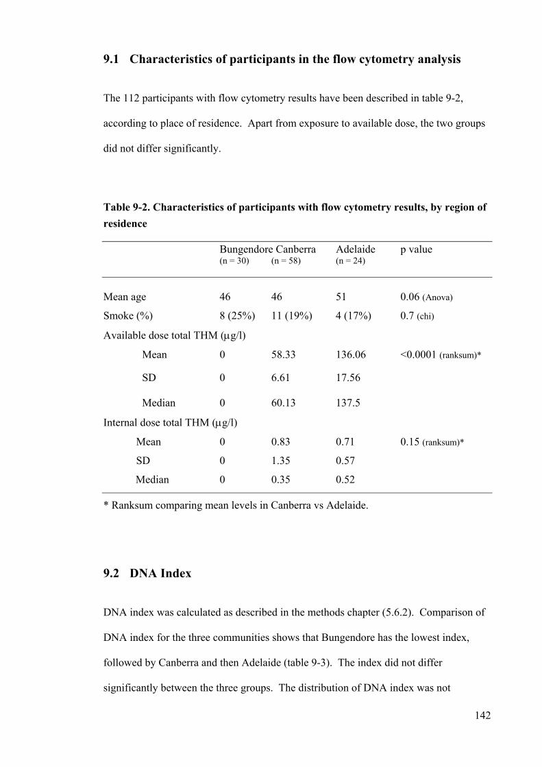
9.1 Characteristics of participants in the flow cytometry analysis

The 112 participants with flow cytometry results have been described in table 9-2,

according to place of residence. Apart from exposure to available dose, the two groups

did not differ significantly.

Table 9-2. Characteristics of participants with flow cytometry results, by region of residence

Bungendore Canberra Adelaide p value (n = 30) (n = 58) (n = 24) Mean age 46 46 51 0.06 (Anova)

Smoke (%) 8 (25%) 11 (19%) 4 (17%) 0.7 (chi)

Available dose total THM (µg/l)

Mean 0 58.33 136.06 <0.0001 (ranksum)*

SD 0 6.61 17.56

Median 0 60.13 137.5

Internal dose total THM (µg/l)

Mean 0 0.83 0.71 0.15 (ranksum)*

SD 0 1.35 0.57

Median 0 0.35 0.52

* Ranksum comparing mean levels in Canberra vs Adelaide.

9.2 DNA Index

DNA index was calculated as described in the methods chapter (5.6.2). Comparison of

DNA index for the three communities shows that Bungendore has the lowest index,

followed by Canberra and then Adelaide (table 9-3). The index did not differ

significantly between the three groups. The distribution of DNA index was not

142

normally distributed, and was transformed to a normal distribution by log

transformation. All analysis undertaken with DNA index utilises log-transformed

values.

Table 9-3. DNA index (untransformed) by region of residence

Mean SD Median Range

Bungendore (n=30) 4.40 3.89 3.70 0.68 to 18.66

Canberra (n=58) 8.61 19.58 3.59 0.50 to 138.6

Adelaide (n=24) 8.81 8.36 5.92 0.92 to 36.78

p = 0.06*/ 0.07**

* anova of log transformed DNA index, comparing the three groups

** ttest comparing Bungendore (unexposed) vs Canberra/Adelaide (exposed)

Examining the relationship between exposure and DNA index from flow cytometry was

undertaken using multiple regression models. The steps in identifying interaction terms

and confounding variables for inclusion in the models were the same as for the Poisson

regression model described in the previous chapter.

9.3 Association between THM and DNA index

Exposure levels in terms of available dose and internal dose were plotted against DNA

index to examine for linear or non-linear patterns of relationship. No obvious

relationship was visible (appendices 1a and 3a).

The association between exposure and outcome was assessed using a multiple

regression model, adjusting for interaction and confounding. Identifying highly

143

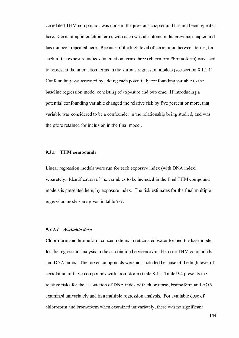
correlated THM compounds was done in the previous chapter and has not been repeated

here. Correlating interaction terms with each was also done in the previous chapter and

has not been repeated here. Because of the high level of correlation between terms, for

each of the exposure indices, interaction terms three (chloroform*bromoform) was used

to represent the interaction terms in the various regression models (see section 8.1.1.1).

Confounding was assessed by adding each potentially confounding variable to the

baseline regression model consisting of exposure and outcome. If introducing a

potential confounding variable changed the relative risk by five percent or more, that

variable was considered to be a confounder in the relationship being studied, and was

therefore retained for inclusion in the final model.

9.3.1 THM compounds

Linear regression models were run for each exposure index (with DNA index)

separately. Identification of the variables to be included in the final THM compound

models is presented here, by exposure index. The risk estimates for the final multiple

regression models are given in table 9-9.

9.3.1.1 Available dose

Chloroform and bromoform concentrations in reticulated water formed the base model

for the regression analysis in the association between available dose THM compounds

and DNA index. The mixed compounds were not included because of the high level of

correlation of these compounds with bromoform (table 8-1). Table 9-4 presents the

relative risks for the association of DNA index with chloroform, bromoform and AOX

examined univariately and in a multiple regression analysis. For available dose of

chloroform and bromoform when examined univariately, there was no significant

144

increase in DNA damage, as estimated by DNA index. AOX when examined

univariately indicates a significant association with DNA index, however when included

with chloroform and bromoform in a multiple regression model, this significance is lost.

Table 9-4. Unadjusted relative risks for the association between available dose of

THMs (exposure) and DNA index from flow cytometry

Exposure variable(s) Crude (unadjusted) (n=112) Relative risk 95% confidence interval

* Chloroform 1.003 0.996 to 1.011

* Bromoform 1.031 0.999 to 1.065

* AOX 1.002 1.0002 to 1.007

** Chloroform, 0.9996 0.982 to 1.017

Bromoform, and 1.01 0.94 to 1.09

AOX 1.001 0.997 to 1.006


** multiple regression with three exposure variables

Interaction term three did not demonstrate a significant effect (p=0.57, likelihood-ratio

test), and was therefore not retained for the final model. Introducing the potentially

confounding variables did not alter the relative risk estimates by more than 1% as

shown in appendix 17. Therefore, only age and smoking were included in the multiple

regression models, for reasons explained in section 5.11. Adjusted relative risks are

presented in table 9-9.

145

9.3.1.2 Intake dose estimated by fluid intake diary

When exposure was measured as intake dose (estimated by fluid intake diary), the

relative risk for DNA damage by DNA index was not significant whether examined

univariately or in a multiple regression model (table 9-5). Introducing interaction term

three did not demonstrate a significant effect (p=0.9), and was therefore not retained for

the final model. The potential confounders contributed very little (less than one

percent) towards the association (appendix 18). None of these variables were therefore

retained for the model, and once again, only age and smoking were included in the final

regression model. The adjusted relative risks are presented in table 9-9.

Table 9-5. Unadjusted relative risks for the association between intake dose of

THMs as estimated by fluid intake diary (exposure), and DNA index from flow

cytometry

Exposure variable(s) Crude (unadjusted)

(n=112) Relative risk 95% confidence interval

* Chloroform 1.002 0.999 to 1.005

* Bromoform 1.006 0.832 to 1.031

** Chloroform and 1.002 0.999 to 1.005

Bromoform 1.006 0.998 to 1.030


** Complex mixture model with two or more compounds

9.3.1.3 Intake dose estimated by questionnaire

Table 9-6 below presents relative risk estimates for DNA index examined against

available dose of chloroform and bromoform estimated by questionnaire. As with the

above exposure indices, the relative risk estimates does not support increased DNA

146

damage to bladder cells. The interaction effect did not demonstrate a significant effect

(likelihood-ratio test p=0.4). Introducing the potentially confounding variables made

minimal contribution to the association (appendix 19.).

Table 9-6. Unadjusted relative risks for the association between intake dose of

THMs as estimated by questionnaire (exposure) and DNA index from flow

cytometry



* Chloroform 1.002 0.997 to 1.004

* Bromoform 0.999 0.960 to 1.040

** Chloroform and 1.000 0.997 to 1.004

Bromoform 0.999 0.960 to 1.040



9.3.1.4 Internal dose

The baseline model for internal dose of THMs included concentrations of chloroform,

bromodichloromethane, and bromoform in urine (see section 8.1.1.4 and table 8-10).

Examining these compounds univariately or as a complex mixture did not support

evidence of increased DNA damage (measured by DNA index) with exposure to THMs

(table 9-7). However, similar to the picture seen when micronuclei frequency was used

as the outcome measure, the confidence intervals were somewhat wider than what was

obtained with other exposure measures.

147

Table 9-7. Unadjusted relative risks for the association between internal dose of

THMs (exposure) and DNA index from flow cytometry



* Chloroform 1.06 0.55 to 2.05

* Bromodichloromethane 1.13 0.50 to 2.55

* Bromoform 1.04 0.81 to 1.34

** Chloroform, 1.04 0.53 to 2.04

bromodichloromethane, and 1.11 0.48 to 2.54

Bromoform 1.04 0.80 to 1.34



The interaction term did not result in a change to the association of 5% or more, and

was therefore not retained for the final regression model. Several of the potential

confounders however resulted in changing the association by 5% or more (appendix

20). These variables (Family history of bladder cancer, ever worked with dyes,

chemicals, and truck driver, lifetime history of using dyes in hobbies, or using dyes in a

hobby in the last year, ever working with leather as part of a hobby, Using paint in non-

work related activity in the last fortnight, ever smoked tobacco, exposure to passive

smoking in home environment, swimming in chlorinated water during the study period,

and plasma folate level) were retained for inclusion in the multiple regression model.

148

9.3.2 Total THM

The following table summarises the relative risks, unadjusted for interaction terms or

confounders, for the four exposure indices (table 9-8). Although the relative risk for

exposure measured as available dose total THM was small, this association appeared

significant, while none of the other exposure measures showed a significant increase in

DNA damage to bladder cells with exposure to total THM.

Table 9-8. Unadjusted relative risks for the association between total THM and

DNA index from flow cytometry, by exposure index

Exposure measure Crude (unadjusted) (n=112) Relative risk 95% confidence interval

Available dose 1.004 1.0004 to 1.0079 Intake dose by diary 1.001 0.999 to 1.003 Intake dose by questionnaire 1.00007 0.997 to 1.003 Internal dose 1.03 0.86 to 1.22

Introducing potentially confounding variables to the various baseline models did not

result in a change in the association by five percent or more for any of the exposure

indices of total THM, and were therefore not retained for the final regression models

(appendix 21). Having identified the variables for inclusion in the final models, a

multiple regression analysis was undertaken to quantify the association between THMs

and DNA index from flow cytometry. In all models, smoking during study period and

age were included as potential confounders. Table 9-9 below presents the findings from

these analyses.

149

Table 9-9. Relative risk for DNA damage to bladder cells (estimated by DNA

index from flow cytometry), with exposure to THMs in community water supplies,

by exposure index, adjusted for interaction and confounding

n=112 Relative risk* 95% confidence interval

Available dose

Chloroform, 0.999 0.982 to 1.017

Bromoform, and 1.01 0.94 to 1.09

AOX 1.01 0.997 to 1.006

Total THM 1.0042 1.0003 to 1.0081

Intake dose by diary

Chloroform and 1.002 0.999 to 1.005

Bromoform 1.003 0.978 to 1.029

Total THM 1.001 0.999 to 1.003

Intake dose by questionnaire

Chloroform and 1.0005 0.997 to 1.004

Bromoform 0.994 0.953 to 1.037

Total THM 1.00008 0.997 to 1.003

Internal dose (n=107)

Chloroform, 1.38 ** 0.64 to 2.97

Bromodichloromethane, and 1.81 ** 0.71 to 4.65

Bromoform 0.97 ** 0.74 to 1.25

Total THM 1.03 0.87 to 1.23

*Adjusted for age and smoking during the study period ** Also adjusted for family history of bladder cancer, ever worked with dyes, chemicals, ever worked as a truck driver, lifetime history of using dyes in hobbies, ever worked with leather as part of a hobby, worked using paint in non-work related activity in the last fortnight, ever smoked tobacco, exposure to passive smoking in home environment, swimming in chlorinated water during the study period and plasma folate level. 150

Chapter 10. Discussion

The risk of developing cancer with exposure to by-products of chlorination is of

significant public health concern because of the large numbers of people the world over

who use chlorinated water for drinking and domestic purposes. This study examines the

association between exposure to DBPs (indicated by THMs levels), and DNA damage

to bladder cells. It overcomes some of the limitations of the earlier studies by obtaining

individual measures of exposure prospectively. It also overcomes the difficulty of

measuring long-term (chronic) exposure by using a pre-clinical biomarker of

genotoxicity to predict the carcinogenic potential of THMs.

The results from this study do not demonstrate a significant association between

exposure to THMs from community water supplies, and DNA damage to bladder

epithelial cells. Of the twenty regression models undertaken to examine the association

between the various exposure measures and DNA damage (estimated by prevalence of

micronuclei or DNA index from flow cytometry), one model (examining available dose

of total THM with DNA index) revealed a significant risk estimate, while all others

were insignificant. A one in twenty significant finding is likely to be a chance

occurrence, and is unlikely to demonstrate a true association. It must be emphasised

that the null findings in this study are for THM levels that were within the Australian

guideline levels for drinking water. The findings cannot be therefore generalised to

THM levels that exceed guideline levels.

151

10.1 Precision and validity of study

Selection of study groups and sampling are important factors that contribute to precision

of a study. This, being a prospective cohort study, is less subject to sampling errors

commonly associated with case-control studies. However, cohort studies are not free of

random error. This cohort study was composed of three communities, and although the

groups did not differ in many of the attributes examined, there may be differences

between the groups that could distort the association under study. All attempts were

made to identify and adjust for factors (such as relevant medical history, occupational

and recreational exposure to chemicals, dyes etc.) that are known to confound the

association.

One important difference between the communities was the water source. Bungendore

water was from a groundwater source whereas water supplies in Canberra and Adelaide

were derived from surface water. Surface water is more susceptible to contamination by

organic matter or potentially carcinogenic pollutants compared to groundwater, and may

therefore exhibit more mutagenic properties. Such an effect, if present, would have

resulted in a bias away from the null, and is therefore unlikely to have been a significant

source of bias in this study.

152

Sample size is another factor that contributes to precision of a study of this kind. The

sample size for this study was based on prevalence of micronuclei in exfoliated bladder

epithelial cells with exposure to arsenic [103]. The desired sample size was achieved

and we can be confident that there was adequate power to detect an association with the

estimates for available dose (i.e. concentration of THM in reticulated water) and intake

dose (which is derived from available dose). The wide confidence intervals around the

risk estimates for internal dose suggest lack of power. This is possibly due to the much

lower concentrations at which THMs occur in urine compared to water. At such low

concentrations, detecting an effect would require larger numbers. Lack of power for the

internal dose analysis would also explain the widening of confidence intervals when

outliers were excluded from the analysis. Excluding outliers reduced the number of

observations in the multiple regression analysis from 577 (n=214) to 512 (n=190)

observations. The risk estimates for internal dose are less robust.

Sampling within the groups is also a potential source of bias that needs to be considered.

In Bungendore, no sampling was done, and all eligible persons in Bungendore were

asked to participate. In Canberra and Adelaide, areas with higher THMs levels in

reticulated water were identified, and within each area, a strict random sample was

selected. In all three communities, households were identified from telephone

directories. This would lead to exclusion of people at the two extremes of the socio-

economic scale because of the exclusion of those without telephone connections and

those with silent numbers. The selection enables us to broadly generalise about the

issue on which the cohort was chosen – level of exposure to THMs in community water.

Selection bias results from the sample completing the study not being representative of

the population under study. No information is available on persons who were eligible

but not willing to participate, and a comparison of this group with those who

participated cannot be made to determine if the two groups differed.

A strength of this study was the detailed exposure measures obtained at an individual

level. In addition, three indices of exposure were obtained for each participant, and

exposure from ingestion, dermal and inhalation was considered. It is recognised that

dermal and inhalation exposure was computed using estimated shower air concentration

153

(based on experimental models). It is unlikely that a resulting error in the estimated

dermal or inhalation exposure would make a significant difference to the final risk

estimate. This is the first study (to our knowledge) that has even attempted to estimate

dermal and inhalation exposure.

Contributing to the precision of exposure measure were the standards associated with

THM testing. THM assays for this study were carried out by two laboratories that were

accredited by the National Association of Testing Authorities, Australia (NATA), and

are therefore required to comply with national standards.

The study presented here is limited to exploring the suitability of non-invasive exposure

measures (i.e. in water and urine) to assess genotoxicity of chlorine disinfected water

supplies. Blood concentrations of THMs may have provided a more accurate measure

of internal dose, although assay of volatile compounds in blood is also prone to loss of

compounds during collection and analysis. This was not however investigated in this

study. When measuring volatile organic compounds, the loss of compounds through

evaporation must be considered. Due to the semi volatile nature of THMs, it is

recognised that there could be a non-measurable loss of compound on collection and

handling of urine samples, resulting in lower than actual readings. However, urinary

concentration of chloroform has been shown to increase following exposure from

swimming in chlorinated pools, with at least 3-7% of chloroform being secreted via

urine [104].

The failure to adjust the urine THM concentrations in this study for urine volume and

urinary creatinine may have affected the validity of urinary THM concentration as a

measure of internal dose.

154

Non-differential misclassification of outcome also needs to be considered as a possible

explanation for the null findings, as it can produce a bias towards the null. This raises

the matter of validity of the outcome measure, micronuclei.

Micronuclei prevalence has been used successfully to assess genotoxicity of potential

carcinogens such as arsenic, benzene, radiation and smoking [64], [66], [105], [88],

[106], [103], [63], [107], [75]. Micronuclei are a pre-clinical stage in the pathway to

cancer development and it is therefore a biologically plausible outcome measure to

predict carcinogenic potential of a substance.

Preparation of urothelial cells for scoring requires basic laboratory skills with some

specific training. Any effects of the preparation technique for this study would be

randomised across the three study groups as the cells were prepared by the one person,

and is therefore unlikely to result in differential error. Scoring of micronuclei is a

tedious activity and is a subjective process leaving room for error. If specimens from

the various exposure groups are randomly assigned to scorers, or if one scorer does all

the scoring, this error would not contribute to a systematic misclassification. In this

study, there were two scorers, and each scorer kept a record of the position of cells with

micronuclei. An experienced scorer verified a ten percent sample. It is therefore

unlikely that a differential error would result from scoring. Scorers were blind to the

exposure status of participants. Therefore, a diagnostic bias (resulting in differential

misclassification of outcome) was unlikely.

The accuracy of micronuclei assay can be influenced by the number of cells scored,

with random variation having a significant effect if less than 500 cells per participant

155

are scored. Accuracy is said to increase and stabilise when 1500 – 2000 cells per

participant are scored [61]. In this study, the unexposed group had on average 929 cells

per participant, scored. In the two exposed groups, the average number of cells scored

was 463. This is likely to lead to a bias towards the null, and therefore constitutes a

major weakness of this study. However, the fact that flow cytometry analysis, which

is an automated process that was set to pick up 50,000 particles, also revealed similar

results adds confirmatory strength to the null findings of this study.

Flow cytometry technique is less subject to measurement bias compared to the

micronuclei assay. When assessed at an ecological level (comparing results between

study sites), the borderline significantly higher DNA index from flow cytometry among

the exposed group compared to the unexposed group, provides weak evidence that

exposure to chlorinated water may be associated with increased DNA damage to

bladder cells (table 9-3). Given that an association with THM levels was not

demonstrated, it is possible that one of the other potentially carcinogenic substances in

chlorinated water (such as MX Furanone or any of the other DBPs) may be contributing

to this suggestion of increased DNA damage observed by flow cytometry. This

assessment is however subject to the considerable weaknesses of ecological

comparisons.

Flow cytometry was used as an additional outcome measure because it was automated

and fast. There is little or no literature on the use of flow cytometry to quantify DNA

damage in exfoliated epithelial cells, as was used in this study. Exfoliated cells are cells

that have been shed from the epithelium, and are no longer healthy living cells. The fact

that the results obtained were very similar to those obtained with micronuclei possibly

suggests that flow cytometry may prove a suitable option for assessing DNA damage

156

even in exfoliated epithelial cells. A decision on the suitability of the test cannot be

based on a single study, and further investigation of this approach is desirable.

Adding to the strengths of the study was that unlike with animal experimental studies,

participants were exposed to the complex mixture of compounds present in chlorinated

water. Therefore, although the analysis was undertaken in relation to THM levels in the

water, the measured DNA damage to bladder cells was the effect of exposure to the

complex mixture. This effect will be well observed in a follow-up study that was

undertaken in October / November 1999 after chlorination of Bungendore water supply

in May 1999, in which Canberra was the control group. Water samples were obtained

from the reticulation system in Bungendore and Canberra, and participants were asked

to provide urine samples for THM assay and scoring of micronuclei cells. The results

of the follow up study are pending. If this follow-up study demonstrates that the

(unadjusted) prevalence of micronuclei in Bungendore has risen compared to Canberra,

this would indicate that by-products of chlorination have had a genotoxic effect on

bladder cells.

10.2 Implications for the water industry

This study utilised THM concentrations (in water and urine) as the exposure measure.

THMs are routinely monitored DBPs in chlorinated water supplies the world over, and

in the case of smaller water utilities are the only DBP to be monitored. Keeping in mind

the limitations identified, the failure to demonstrate a genotoxic effect on bladder cells

with exposure to THMs, supports recent suggestions that THMs (chloroform in

particular) are not genotoxic, and that the mode of action is cell death from mechanisms

other than DNA damage [4], [108], [48], [109].

157

It is known that THMs are not the most mutagenic compound, and that there are

compounds such as MX Furanone that account for a large proportion of the

mutagenicity of chlorinated water. Given the null findings from this study for an

association between exposure to THMs and genotoxic changes to bladder cells, the next

step in assessing carcinogenicity of DBP in chlorinated waters should be to examine the

relationship between THMs and the more mutagenic compounds. If THM levels

correlate well with the mutagenic compounds in water, THMs may serve as a surrogate

marker for cancer risk from DBP, and the null findings of this study are reassuring for

the water industry. However, no published information was accessible to determine the

correlation. From discussions with experts in the water industry, it appears that water

rich in dissolved organic matter that have been shown to have relatively higher levels of

MX Furanone, tend to have higher levels of THMs. But the correlation between MX

and THM is not established and at this stage, it is not possible to determine the

occurrence of MX based on THM levels alone.

If it is demonstrated that THM levels in treated water do not correlate well with the

more mutagenic compounds, the next step would be to assess the association between

MX Furanone and DNA damage to bladder cells. Although it is recognised that such a

study would be rather costly, it would be of great benefit to the water industry. If an

association is demonstrated between exposure to MX Furanone and genotoxic changes

to bladder cells, this would suggest the need to identify more appropriate predictors of

carcinogenic potential to be monitored in chlorinated water. It is worth noting at this

stage that it was originally intended to measure MX Furanone levels in this study, but

the associated cost made this not feasible.

158

Identifying a suitable indicator for assessing health risks associated with chemicals in

water is important to obtain a balance between microbial and chemical risks. The lack

of consensus on guideline levels or maximum admissible concentrations, compounded

by the fear of cancer with chemical use, has led to much uncertainty, and a trend

towards decreasing chemical standards by regulatory authorities. Alterations in

treatment processes need to be judged carefully to ensure continued microbial safety of

drinking water. The continuing occurrence of water borne disease outbreaks in the

industrial countries as illustrated by a few recent reports, are a constant reminder of the

possible public health consequences of transient water supply contamination [110],

[111], [112], [113], [114]. It is therefore essential that the water treatment process be

carefully monitored, and an appropriate indicator for health risk assessment from

chemical disinfection be identified.

Whatever the final conclusion is in regard to the cancer risk associated with DBP in

chlorinated water, we need to recognise that at the present time, chlorine is the most

cost-effective method of disinfecting large community water supplies. This measure

had an enormous public health impact by reducing water-borne disease transmission.

Alternative disinfection methods have their own problems. Ozone provides no residual

disinfection and generates different by-products (such as aldehydes, glyoxals,

formaldehydes, and brominated compounds) that are also toxic. It is also costly to

implement, and by itself does not provide residual disinfection [5]. Chlorine dioxide is

a powerful disinfectant with no THM formation [115], [116]. It is by itself toxic, and

generates toxic by-products similar to those of ozone. Chloramination is a less powerful

biocide than chlorine, ozone or chlorine dioxide, but it retains activity for longer periods

of time, and therefore ideal for situations where low residual levels are require. Ultra

violet radiation disinfects by disrupting the chemical bonds of many molecules. It has

159

been found to be effective in water treatment, especially when used in conjunction with

activated carbon filtration, but it provides no residual disinfection effect [117].

Therefore, it is important that all effort be put in to maximising the benefits from

chlorination.

10.3 Conclusion

This study has not demonstrated an association between exposure to THMs from

chlorinated water and DNA damage to bladder epithelial cells. While this is reassuring

to the water industry, this study needs to be supplemented by studies correlating THM

levels with the other more mutagenic compounds such as MX Furanone in chlorinated

drinking water. If there is no strong correlation between THMs and these compounds,

studies will then be needed to examine the association between exposure to these

mutagenic compounds and DNA damage to bladder cells. Such information is

important for the development of drinking water guidelines that are currently focused on

THMs.

The possibility of an association between THMs and DNA damage to bladder cells

should be further explored in populations with exposure to higher THM levels.

160

Documents

Chapter 6. Results - ANU · Chapter 6. Results A total of 1233 recruitment letters were mailed, and 529 persons were identified as being eligible to participate. Of these, 348 (65.8%)