Embed Size (px)
Citation preview

Chapter 6
Propagation
Al Penney
VO1NO
1

ObjectivesTo become familiar with:
– Classification of waves wrt propagation;
– Factors that affect radio wave propagation; and
– Propagation characteristics of Amateur bands.
Propagation
– How signals get from Point A to Point B.
Al Penney
VO1NO
2

Waves• Transverse
– Vibration is at right angles to direction of propagation, e.g.: guitar string
• Longitudinal
– Vibration is parallel to direction of propagation, e.g.: sound waves
Al Penney
VO1NO
3

Electromagnetic (EM) Waves
• Transverse waves
• Consist of Electric and Magnetic components:
– In phase with each other; and
– At right angles to each other.
• Orientation of Electric field determines Polarization.
Al Penney
VO1NO
4
Al Penney
VO1NO
5

Classification of Waves
Direct
(VHF, UHF)
ReflectedSurface or Ground Wave
(VLF, LF, MF, HF)
Skywave (HF)
AKA Ionospheric Wave
Ionosphere
Al Penney
VO1NO
6

Classification of WavesRadio Waves
Space Waves Ground Waves
Skywave Reflected Direct Surface
Al Penney
VO1NO
space waves are the radio waves of very high frequency (i.e. between 30
MHz to 300 MHz or more). The space waves can travel through atmosphere
from transmitter antenna to receiver antenna either directly or after reflection from ground in the earth's stratosphere region.
In radio communication, skywave or skip refers to the propagation of radio
waves reflected or refracted back toward Earth from the ionosphere,
an electrically charged layer of the upper atmosphere. Since it is not limited by
the curvature of the Earth, skywave propagation can be used to communicate beyond the horizon, at intercontinental distances. It is mostly used in
the shortwave frequency bands.
As a result of skywave propagation, a signal from a distant AM
broadcasting station, a shortwave station, or – during sporadic E
propagation conditions (principally during the summer months in both
hemispheres) a distant VHF FM or TV station – can sometimes be received as
clearly as local stations. Most long-distance shortwave (high frequency) radio communication – between 3 and 30 MHz – is a result of skywave propagation.
Since the early 1920s amateur radio operators (or "hams"), limited to lower
transmitter power than broadcast stations, have taken advantage of skywave
for long-distance (or "DX") communication.

Skywaves also called Ionospheric Waves.
Reflected waves are those reflected off terrain.
The term ground wave has had several meanings in antenna literature, but it has come
to be applied to any wave that stays close to the Earth, reaching the receiving point
without leaving the Earth’s lower atmosphere. This distinguishes the ground wave
from a sky wave, which utilizes the ionosphere for propagation between the
transmitting and receiving antennas. The ground wave could be traveling in actual
contact with the ground, as in Fig 1, where it is called the surface wave. Or it could
travel directly between the transmitting and receiving antennas, when they are high
enough so they can “see” each other—this is commonly called the direct wave. The
ground wave also travels between the transmitting and receiving antennas by
reflections or diffractions off intervening terrain between them. The ground-
influenced wave may interact with the direct wave to create a vector-summed
resultant at the receiver antenna.
THE SURFACE WAVE
The surface wave travels in contact with the Earth’s surface. It can provide coverage
up to about 100 miles in the standard AM broadcast band during
the daytime, but attenuation is high. The attenuation increases with frequency.
The surface wave is of little value in amateur communication, except possibly at 1.8
MHz and the 630 Meter Band. Vertically polarized antennas must be used, which
tends to limit amateur surface-wave communication to where large vertical systems
can be erected.
Ground wave refers to the propagation of radio waves parallel to and adjacent
to the surface of the Earth.
Surface Wave propagation works because lower-frequency waves are more strongly diffracted around obstacles due to their long wavelengths, allowing
them to follow the Earth's curvature. Ground waves propagate in vertical
polarization, with their magnetic field horizontal and electric field (close to)
vertical. With VLF waves, the ionosphere and earth's surface act as
a waveguide.
Conductivity of the surface affects the propagation of surface waves, with more
conductive surfaces such as sea water providing better
7

propagation. Increasing the conductivity in a surface results in less
dissipation. The refractive indices are subject to spatial and temporal changes.
Since the ground is not a perfect electrical conductor, ground waves are
attenuated as they follow the earth's surface. The wavefronts initially are
vertical, but the ground, acting as a lossy dielectric, causes the wave to tilt
forward as it travels. This directs some of the energy into the earth where it is dissipated,[15] so that the signal decreases exponentially.
Most long-distance LF "longwave" radio communication (between 30 kHz and
300 kHz) is a result of groundwave propagation. Mediumwave radio
transmissions (frequencies between 300 kHz and 3000 kHz), including AM
broadcast band, travel both as groundwaves and, for longer distances at night,
as skywaves. Ground losses become lower at lower frequencies, greatly
increasing the coverage of AM stations using the lower end of the band.
The VLF and LF frequencies are mostly used for military communications,
especially with ships and submarines. The lower the frequency the better the waves penetrate sea water. ELF waves (below 3 kHz) have even been used to
communicate with deeply submerged submarines.
Ground waves have been used in over-the-horizon radar, which operates
mainly at frequencies between 2–20 MHz over the sea, which has a sufficiently
high conductivity to convey them to and from a reasonable distance (up to 100 km or more; over-horizon radar also uses skywave propagation at much
greater distances). In the development of radio, ground waves were used
extensively. Early commercial and professional radio services relied exclusively on long wave, low frequencies and ground-wave propagation. To
prevent interference with these services, amateur and experimental
transmitters were restricted to the high frequencies (HF), felt to be useless
since their ground-wave range was limited. Upon discovery of the other propagation modes possible at medium wave and short wave frequencies, the
advantages of HF for commercial and military purposes became apparent.
Amateur experimentation was then confined only to authorized frequencies in
the range.
Direct modes (line-of-sight)Line-of-sight refers to radio waves which
travel directly in a line from the transmitting antenna to the receiving antenna.
It does not necessarily require a cleared sight path; at lower frequencies radio
waves can pass through buildings, foliage and other obstructions.
7

Surface or Ground Waves
• Wave front slows near Earth, bending it down.
• Signal “hugs” the Earth.
• For lower frequency bands – 630, 160, and 80M.
• Good for ~ 200 km by day.
• Range rapidly decreases for higher frequency bands.
• Best over high conductivity terrain – sea water best.Al Penney
VO1NO
Ground wave propagation is particularly important on the LF and MF portionof the radio spectrum. Ground wave radio propagation is used to provide
relatively local radio communications coverage, especially by radio broadcast
stations that require to cover a particular locality.
Ground wave propagation of radio signal is ideal for relatively short distance
propagation on these frequencies during the daytime. Sky-wave ionospheric
propagation is not possible during the day because of the attenuation of the
signals on these frequencies caused by the D region in the ionosphere. In view
of this, radio communications stations need to rely on the ground-wave
propagation to achieve their coverage.
The surface wave is also very dependent upon the nature of the ground over
which the signal travels. Ground conductivity, terrain roughness and the
dielectric constant all affect the signal attenuation. In addition to this the
ground penetration varies, becoming greater at lower frequencies, and this
means that it is not just the surface conductivity that is of interest. At the
higher frequencies this is not of great importance, but at lower frequencies
penetration means that ground strata down to 100 meters may have an effect.
Despite all these variables, it is found that terrain with good conductivity gives
the best result. Thus soil type and the moisture content are of importance.
Salty sea water is the best, and rich agricultural, or marshy land is also good.Dry sandy terrain and city centers are by far the worst. This means sea paths

are optimum, although even these are subject to variations due to the
roughness of the sea, resulting on path losses being slightly dependent upon
the weather. It should also be noted that in view of the fact that signal
penetration has an effect, the water table may have an effect dependent upon
the frequency in use.
8

Al Penney
VO1NO
Marconi believed that radio waves would follow the earth's curvature, making communication to ships at sea feasible, and designed an experiment to prove his contention.
In December 1901 Marconi assembled his receiver at Signal Hill, St. John's, nearly the closest point to Europe in North America. He set up his receiving apparatus in an abandoned hospital that straddled the cliff facing Europe on the top of Signal Hill. After unsuccessful attempts to keep an antenna aloft with balloons and kites, because of the high winds, he eventually managed to raise an antenna with a kite for a short period of time for each of a few days. Accounts vary, but Marconi's notes indicate that the transatlantic message was received via this antenna.
At the appointed time each day his staff in Poldhu transmitted the Morse code letter "s" - three dots. This signal had been chosen as the most easily distinguished. On the 12 December Marconi pressed his ear to the telephone headset of his rudimentary receiver and successfully heard "pip, pip, pip" - slightly more than 2100 miles from the transmitter. This demonstrated that transatlantic wireless communication was possible. While "ground waves" followed the curvature of the earth for only a short distance over the horizon, "sky waves" also bounced off the ionosphere in the upper atmosphere and returned to earth, which although unknown at the time, had allowed Marconi to demonstrate that radio communication over great distances was possible.
Although Marconi had proved that radio transmissions could be received well beyond line of sight, he was not aware of the mechanism that permitted it – the Ionosphere.
9

Ionosphere• 50 to 600 km above Earth’s surface.
• Atmosphere very thin.
• Ultraviolet (UV) light, X-rays and cosmic radiation from Sun ionize molecules and atoms, a process called Ionization.
• Ionized particles concentrate into 4 distinct layers – D, E, F1 and F2.
• Layers change density and height due to Recombination.
Al Penney
VO1NO
The ionosphere is the ionized part of Earth's upper atmosphere, from about
60 km (37 mi) to 1,000 km (620 mi) altitude, a region that includes
the thermosphere and parts of the mesosphere and exosphere. The
ionosphere is ionized by solar radiation. It plays an important role
in atmospheric electricity and forms the inner edge of the magnetosphere. It
has practical importance because, among other functions, it influences radio
propagation to distant places on the Earth

Ionization
Recombination
Al Penney
VO1NO
Ionization or ionisation, is the process by which an atom or a molecule
acquires a negative or positive charge by gaining or losing electrons, often in
conjunction with other chemical changes. The resulting electrically charged atom or molecule is called an ion. Ionization can result from the loss of an
electron after collisions with subatomic particles, collisions with other atoms,
molecules and ions, or through the interaction with electromagnetic radiation.

Al Penney
VO1NO
Due to the ability of ionized atmospheric gases to refract high frequency (HF,
or shortwave) radio waves, the ionosphere can reflect radio waves directed
into the sky back toward the Earth. Radio waves directed at an angle into the
sky can return to Earth beyond the horizon. This technique, called "skip" or
"skywave" propagation, has been used since the 1920s to communicate at
international or intercontinental distances. The returning radio waves can
reflect off the Earth's surface into the sky again, allowing greater ranges to be achieved with multiple hops. This communication method is variable and
unreliable, with reception over a given path depending on time of day or night, the seasons, weather, and the 11-year sunspot cycle. During the first half of
the 20th century it was widely used for transoceanic telephone and telegraph
service, and business and diplomatic communication. Due to its relative
unreliability, shortwave radio communication has been mostly abandoned by
the telecommunications industry, though it remains important for high-latitude
communication where satellite-based radio communication is not possible. Some broadcasting stations and automated services still use shortwave
radio frequencies, as do radio amateur hobbyists for private recreational
contacts.

D Layer• Innermost layer.
• Approximately 50 – 80km altitude.
• Dense in daylight, disappears at night.
• Not useful for long-distance propagation.
• Absorbs signals below approximately 10 MHz.
Al Penney
VO1NO
D layerThe D layer is the innermost layer, 60 km (37 mi) to 90 km (56 mi) above the surface of the Earth. Ionization here is due to Lyman series-alpha hydrogen radiation at a wavelength of 121.5 nanometre (nm) ionizing nitric oxide (NO). In addition, with high Solar activity hard X-rays (wavelength < 1 nm) may ionize (N₂, O₂). During the night cosmic rays produce a residual amount of ionization. Recombination is high in the D layer, the net ionization effect is low, but loss of wave energy is great due to frequent collisions of the electrons (about ten collisions every msec). As a result high-frequency (HF) radio waves are not reflected by the D layer but suffer loss of energy therein. This is the main reason for absorption of HF radio waves, particularly at 10 MHz and below, with progressively smaller absorption as the frequency gets higher. The absorption is small at night and greatest about midday. The layer reduces greatly after sunset; a small part remains due to galactic cosmic rays. A common example of the D layer in action is the disappearance of distant AM broadcast band stations in the daytime.During solar proton events, ionization can reach unusually high levels in the D-region over high and polar latitudes. Such very rare events are known as Polar Cap Absorption (or PCA) events, because the increased ionization significantly enhances the absorption of radio signals passing through the region. In fact, absorption levels can increase by many tens of dB during intense events, which is enough to absorb most (if not all) transpolar HF radio signal transmissions. Such events typically last less than 24 to 48 hours.
13
E Layer• First to be discovered.
• Approximately 90 to 120 km altitude.
• Almost disappears at night.
• Usually does not play a part in long distance propagation.
• Sporadic E can reflect signals on 6M and 2M however.
• Auroral activity takes place here.
Al Penney
VO1NO
E layerThe E layer is the middle layer, 90 km (56 mi) to 120 km (75 mi) above the surface of the Earth. Ionization is due to soft X-ray (1-10 nm) and far ultraviolet (UV) solar radiation ionization of molecular oxygen (O₂). Normally, at oblique incidence, this layer can only reflect radio waves having frequencies lower than about 10 MHz and may contribute a bit to absorption on frequencies above. However, during intense Sporadic E events, the Es layer can reflect frequencies up to 50 MHz and higher. The vertical structure of the E layer is primarily determined by the competing effects of ionization and recombination. At night the E layer rapidly disappears because the primary source of ionization is no longer present. After sunset an increase in the height of the E layer maximum increases the range to which radio waves can travel by reflection from the layer.This region is also known as the Kennelly–Heaviside layer or simply the Heaviside layer. Its existence was predicted in 1902 independently and almost simultaneously by the American electrical engineer Arthur Edwin Kennelly (1861–1939) and the British physicist Oliver Heaviside (1850–1925). However, it was not until 1924 that its existence was detected by Edward V. Appleton.
14

F Layer• Highest layer.
• Approximately 150 to 600 km altitude.
• Responsible for most long-distance propagation on HF.
• Often 1 layer at night, breaking into 2 in daylight (F1 and F2).
Al Penney
VO1NO
F layerThe F layer or region, also known as the Appleton layer, extends from about 200 km (120 mi) to more than 500 km (310 mi) above the surface of Earth. It is the densest point of the ionosphere, which implies signals penetrating this layer will escape into space. At higher altitudes, the number of oxygen ions decreases and lighter ions such as hydrogen and helium become dominant; this layer is the topside ionosphere. There, extreme ultraviolet (UV, 10–100 nm) solar radiation ionizes atomic oxygen. The F layer consists of one layer at night, but during the day, a deformation often forms in the profile that is labeled F₁. The F₂ layer remains by day and night responsible for most skywave propagation of radio waves, facilitating high frequency (HF, or shortwave) radio communications over long distances.From 1972 to 1975 NASA launched the AEROS and AEROS B satellites to study the F region.
15

Al Penney
VO1NO
16

Al Penney
VO1NO
Refraction is the bending of a ray as it passes from one medium to another at an angle.
The appearance of bending of a straight stick, where it enters water at an angle, is an
example of light refraction known to us all.
Mechanism of refraction
When a radio wave reaches the ionosphere, the electric field in the wave
forces the electrons in the ionosphere into oscillation at the same frequency as
the radio wave. Some of the radio-frequency energy is given up to this
resonant oscillation. The oscillating electrons will then either be lost to
recombination or will re-radiate the original wave energy. Total refraction can
occur when the collision frequency of the ionosphere is less than the radio
frequency, and if the electron density in the ionosphere is great enough.
A qualitative understanding of how an electromagnetic wave propagates through the ionosphere can be obtained by recalling geometric optics. Since
the ionosphere is a plasma, it can be shown that the refractive index is less
than unity. Hence, the electromagnetic "ray" is bent away from the normal
rather than toward the normal as would be indicated when the refractive index
is greater than unity. It can also be shown that the refractive index of a plasma,
and hence the ionosphere, is frequency-dependent,

Al Penney
VO1NO
The degree of bending of a wave path in an ionized layer depends on the density of
the ionization and the frequency.
The bending at any given frequency or wavelength will increase with increased
ionization density. For a given ionization density, bending will decreases with
frequency. Two extremes are thus possible. If the intensity of the ionization is
sufficient and the frequency low enough, even a wave entering the layer
perpendicularly will be reflected back to Earth. Conversely, if the frequency is high
enough or the ionization decreases to a low enough density, a condition is reached
where the wave angle is not affected enough by the ionosphere to cause a useful
portion of the wave energy to return to the Earth. This basic principle has been used
for many years to “sound” the ionosphere to determine its communication potential at
various wave angles and frequencies.

Al Penney
VO1NO
Because the skywave can be refracted back to Earth a long distance from the transmit antenna, the may be a region between the extent of the ground wave from the antenna to the point where the skywave is first refracted back to Earth where there is no signal.
Skip Zone – The area between the furthest reach of the Ground Wave and the point where the Sky Wave is first refracted back to Earth. No signal is heard in the Skip Zone.
Skip Distance – The minimum distance reached by a signal after refraction or reflection by the Ionosphere.

Skip Zone and Skip Distance
• Skip Zone – The area between the furthest reach of the Ground Wave and the point where the Sky Wave is first refracted back to Earth. No signal is heard in the Skip Zone.
• Skip Distance – The minimum distance reached by a signal after refraction or reflection by the Ionosphere.
Al Penney
VO1NO
Skip Distance
When the critical angle is less than 90 there will always be a region around the
transmitting site where the ionospherically propagated signal cannot be heard, or is
heard weakly. This area lies between the outer limit of the ground-wave range and the
inner edge of energy return from the ionosphere. It is called the skip zone, and the
distance between the originating site and the beginning of the ionospheric return is
called the skip distance. This terminology should not to be confused with ham jargon
such as “the skip is in,” referring to the fact that a band is open for sky-wave
propagation.
The signal may often be heard to some extent within the skip zone, through various
forms of scattering, but it will ordinarily be marginal in strength. When the skip
distance is short, both groundwave and sky-wave signals may be received near the
transmitter. In such instances the sky wave frequently is stronger than the ground
wave, even as close as a few miles from the transmitter. The ionosphere is an efficient
communication medium under favorable conditions. Comparatively, the ground wave
is not.

Al Penney
VO1NO
A
B
Signals that have been refracted back to Earth can also be reflected back up to the ionosphere and be refracted back to earth again. Under the right conditions, this can take place several times, permitting signals to travel completely around the globe.
A radio signal will often be reflected from the reception point on the Earth into the
ionosphere again, reaching the Earth a second time at a still more distant point. As in
the case of light waves, the angle of reflection is the same as the angle of incidence, so
a wave striking the surface of the Earth at an angle of, say, 15 is reflected upward
from the surface at approximately the same angle. Thus, the distance to the second
point of reception will be about twice the distance of the first. Under some conditions
it is possible for as many
as four or five signal hops to occur over a radio path, but no more than two or three
hops is the norm. In this way, HF communication can be conducted over thousands of
miles.
An important point should be recognized with regard to signal hopping. A significant
loss of signal occurs with each hop. The D and E layers of the ionosphere absorb
energy from the signals as they pass through, and the ionosphere tends to scatter the
radio energy in various directions, rather than confining it in a tight bundle. The
roughness of the Earth’s surface also scatters the energy at a reflection point. at greater
distances. It is because of these losses that no more than four or five propagation hops
are useful; the received signal becomes too weak to be usable over more hops.
Although modes other than signal hopping also account for the propagation of radio
waves over thousands of miles, backscatter studies of actual radio propagation have
displayed signals with as many as 5 hops. So the hopping mode is one distinct
possibility for long-distance communication.
21

Ground Wave
Skip Zone
No Signal
First Bounce
Signal Heard
Signal Heard
No Signal
Second Bounce
Skip Distance
2nd Skip Zone
Al Penney
VO1NO
Perfect case – it never actually happens this way because the ionosphere is not uniform around a transmitter, and because of scatter propagation.

Al Penney
VO1NO
It is possible for a signal to take more than one route to get to the receiver. In the
diagram above, lower angle signals will reach the receiver after only one refraction
through the ionosphere. Higher angle signals (assuming they are less than the Critical
angle – the angle above which signals are refracted into space and do not reach Earth)
can be reflected back into the ionosphere and then refracted back to Earth again.
Assuming that both waves do reach point B in the figure above, the low-angle wave
will contain more energy at point B. This wave passes through the lower layers just
twice, compared to the higher-angle route, which must pass through these layers four
times, plus encountering an Earth reflection. Measurements indicate that although
there can be great variation in the relative strengths of the two signals— the one-hop
signal will generally be from 7 to 10 dB stronger. The nature of the terrain at the mid-
path reflection point for the two-hop wave, the angle at which the wave is reflected
from the Earth, and the condition of the ionosphere in the vicinity of all the refraction
points are the primary factors in determining the signal-strength ratio. The loss per
hop becomes significant.

Al Penney
VO1NO
Actual example of propagation ray paths, between Hawaii and West coast. Note refraction from both the E and F layers. The first Skip Zone is distinct, but the next one is not as definite, with some level of signal present. Note also the Critical Angle, above which signals escape into space.

Backscatter• Signals scattered back into Skip Zone.
• Usually associated with operating near the MUF.
• Generally weak and fluttery signals.
• Characteristic “hollow” sounding signals.
• Side- and Forward Scatter are a similar phenomena.Al Penney
VO1NO
F-Layer Backscatter and Sidescatter
Special forms of F-layer scattering can create unusual paths within the skip zone.
Backscatter and sidescatter signals are usually observed just below the MUF for the
direct path and allow communications not normally possible by other means. Stations
using backscatter point their antennas toward a common scattering region at the one-
hop distance, rather than toward each other. Backscattered signals are generally weak
and have a characteristic hollow sound. Useful communication distances range from
100 km (60 mi) to the normal one-hop distance of 4000 km (2500 mi).
Backscatter and sidescatter are closely related and the terminology does not precisely
distinguish between the two. Backscatter usually refers to single-hop signals that have
been scattered by the Earth or the ocean at some distant point back toward the
transmitting station. Two stations spaced a few hundred km apart can often
communicate via a backscatter path near the MUF.
Sidescatter usually refers to a circuit that is oblique to the normal great-circle path.
Two stations can make use of a common side-scattering region well off the direct
path, often toward the south. European and North American stations sometimes
complete 28-MHz contacts via a scattering region over Africa. US and Finnish 50-
MHz operators observed a similar effect early one morning in November 1989 when
they made contact by beaming off the coast of West Africa.

Al Penney
VO1NO
4000 km
2500 Miles
Maximum Distances
Maximum 1-hop distance a signal can reach off F2 layer is 4000 km / 2500 miles (For exam – in reality it can go to ~ 4800 km).
Maximum 1-hop distance a signal can reach off E layer is 2000 km / 1250 miles.
The lower the angle of radiation of the EM wave from the transmit antenna, the further away the signal will travel (assuming it is refracted back to earth).
The higher the refracting layer, the further away the signal will travel (assuming it is refracted back to earth).

28 MHz
3.5 MHz
Al Penney
VO1NO
Lower frequency signals are refracted more for a given level of ionization, meaning the Critical Angle is greater for lower frequencies than higher frequencies. The lower frequency signals return to the ground at closer distances however, meaning that multiple “hops” may be required to reach the target area. This results in weaker signal strength.
Because the lower frequencies are refracted more, the skip distance is less, meaning communications can be established with stations closer to the transmitter than would be possible with higher frequencies.

Skywave Polarization
• Orientation of Electric component of EM Wave.
• Ordinarily TX and RX antennas should have same polarization.
• Faraday Rotation, Refraction and Reflectionchanges polarity of skywaves randomly, so antenna polarization not critical.
• Can cause Fading.
Al Penney
VO1NO
Radio waves passing through the Earth's ionosphere are likewise subject to
the Faraday effect. In conjunction with the earth's magnetic field, rotation of
the polarization of radio waves occurs. Since the density of electrons in the ionosphere varies greatly on a daily basis, as well as over the sunspot cycle,
the magnitude of the effect varies. However the effect is always proportional
to the square of the wavelength, so even at the UHF television frequency of 500 MHz (λ = 60 cm), there can be more than a complete rotation of the axis of
polarization. A consequence is that although most radio transmitting antennas
are either vertically or horizontally polarized, the polarization of a medium or short wave signal after reflection by the ionosphere is rather unpredictable.
However the Faraday effect due to free electrons diminishes rapidly at higher frequencies (shorter wavelengths) so that at microwave frequencies, used
by satellite communications, the transmitted polarization is maintained
between the satellite and the ground.

Solar Cycles
Al Penney
VO1NO
29

Solar Cycle• Periodic change in Sun’s activity and appearance.
• Includes:
– Number of sunspots;
– Level of solar radiation; and
– Ejection of solar material.
• 11 year cycle.
Al Penney
VO1NO
The solar cycle or solar magnetic activity cycle is a nearly periodic 11-year
change in the Sun's activity measured in terms of variations in the number of
observed sunspots on the solar surface. Sunspots have been observed since
the early 17th century and the sunspot time series is the longest, continuously
observed (recorded) time series of any natural phenomena. Accompanying
the 11 year quasi-periodicity in sunspots, the large-scale dipolar (north-south)
magnetic field component of the Sun also flips every 11 years, however, the
peak in the dipolar field lags the peak in the sunspot number, with the former occurring at the minimum between two cycles. Levels of solar radiation and
ejection of solar material, the number and size of sunspots, solar flares,
and coronal loops all exhibit a synchronized fluctuation, from active to quiet to
active again, with a period of 11 years. This cycle has been observed for
centuries by changes in the Sun's appearance and by terrestrial phenomena such as auroras. Solar activity, driven both by the sunspot cycle and transient
aperiodic processes govern the environment of the Solar System planets by
creating space weather and impact space- and ground-based technologies as
well as the Earth's atmosphere and also possibly climate fluctuations on scales
of centuries and longer.
Understanding and predicting the sunspot cycle remains one of the grand
challenges in astrophysics with major ramifications for space science and the understanding of magnetohydrodynamic phenomena elsewhere in the

Universe.
Solar cycles have an average duration of about 11 years. Solar
maximum and solar minimum refer to periods of maximum and minimum
sunspot counts. Cycles span from one minimum to the next.
30

Sunspots• Dark spots on the Sun’s surface.
• Caused by intense magnetic activity that inhibits convection flow of Sun’s interior.
• They host secondary phenomena such as Solar Flares and Coronal Mass Ejections.
Al Penney
VO1NO
Sunspots are temporary phenomena on the photosphere of the Sun that appear visibly as dark spots compared to surrounding regions. They are caused by intense magnetic activity, which inhibits convection by an effect comparable to the eddy current brake, forming areas of reduced surface temperature. They usually appear as pairs, with each sunspot having the opposite magnetic pole to the other.
Although they are at temperatures of roughly 3000–4500 K (2700–4200 °C), the contrast with the surrounding material at about 5,780 K (5,500 °C) leaves them clearly visible as dark spots, as the luminous intensity of a heated black body (closely approximated by the photosphere) is a function of temperature to the fourth power. If the sunspot were isolated from the surrounding photosphere it would be brighter than the Moon. Sunspots expand and contract as they move across the surface of the Sun and can be as small as 16 kilometers (10 mi) and as large as 160,000 kilometers (100,000 mi) in diameter, making the larger ones visible from Earth without the aid of a telescope. They may also travel at relative speeds ("proper motions") of a few hundred meters per second when they first emerge onto the solar photosphere.Manifesting intense magnetic activity, sunspots host secondary phenomena such as coronal loops (prominences) and reconnection events. Most solar flares and coronal mass ejections originate in magnetically active regions around visible sunspot groupings. Similar phenomena indirectly observed on stars are commonly called starspots and both light and dark spots have been measured.[
31

Al Penney
VO1NO
Detailed observations of sunspots have been obtained by the Royal Greenwich
Observatory since 1874. These observations include information on the sizes and
positions of sunspots as well as their numbers. These data show that sunspots do not
appear at random over the surface of the sun but are concentrated in two latitude
bands on either side of the equator. A butterfly diagram (142 kb GIF image) (184 kb
pdf-file) (updated monthly) showing the positions of the spots for each rotation of the
sun since May 1874 shows that these bands first form at mid-latitudes, widen, and
then move toward the equator as each cycle progresses.

33

Solar Cycle 24 has been one of the quietest, weakest cycles in a century. (The prior cycle 23 also had an extended period of very few sunspots.)
SOLAR CYCLE 25 PREDICTIONS
According to NOAA/NASA experts: “Cycle 25 will be similar in size to cycle 24, preceded by a long, deep minimum. Solar Cycle 25 may have a slow start, but is anticipated to peak with solar maximum occurring between 2023 and 2026, and a sunspot range of 95 to 130. This is well below the average number of sunspots, which typically ranges from 140 to 220 sunspots per solar cycle.”
In other words, Solar Cycle

Effect on Propagation• Low solar activity = less ionization;
– Higher frequencies pass through ionosphere into space.
• High solar activity = more ionization;
– Higher frequencies refracted back to earth, and at greater distances.
Al Penney
VO1NO
35

Maximum Usable Frequency
• Known as MUF
• The highest frequency that will be refracted back to Earth by ionized layers over a specified path at a specified time.
• Above this frequency the signals land beyond the station, or travel into space.
• Depends on solar activity, time of day, time of year, and the location of the two stations.
Al Penney
VO1NO
In radio transmission maximum usable frequency (MUF) is the highest radio frequency that can be used for transmission between two points via reflection from the ionosphere ( skywave or "skip" propagation) at a specified time, independent of transmitter power.
MUF and LUF stand respectively for Maximum and Lowest Usable Frequency. These two values define the maximum usable spectrum range in which propagation is open, allowing HF communications, what could be the other perturbations or conditions. It doesn't tell thus all the story as many other "system" factors affect the propagation of sky waves (all parameters that characterize a communication circuit between two stations like the emission power, antenna gain, takeoff angle, QRM, S/N ratio, etc).
The MUF represents the statistical frequency during which a 3000 km-single hop refraction via the F2-layer is generally open 50% of the time. This is thus a median value. That means that you have a 50-50 chance to work in the specified conditions. That means also that sometimes you will only have 1% of chance to work up to that frequency, at another occasion 100% of chance to work it, but nobody can tell you what days are the best. The MUF only tells you that in average 15 days per month the higher frequency will be open as predicted.
Frequencies well below the MUF are affected by the D-layer that shows a strong absorption while the E-layer reflect shortwaves back to earth more often than expected. Above the MUF your chance to make contacts are almost null. Due to their high frequency, sky waves are not more reflected by the F-layers (F2 or F) and escape into space.
Using sky waves it is thus impossible to work on frequencies too away below or above the MUF. The Highest Possible Frequency, HPF, is the upper usable limit exceeded 10% of the time, or 3 days per month, or say in other words, in exceptional conditions. During the 90% of time we use the Frequency of Optimal Transmission (after the French words), aka FOT. It is defined as the statistical frequency during which the MUF can be exceeded of 85% (see below). This range of frequencies spreading between the FOT and the HPF is 4 MHz wide or larger, sometimes so wide that it include two ham bands. To know the probability to use such exceptional conditions, there is only parameter to check in propagation prediction programs : the "required reliability"of the signal-to-noise ratio (SNRxx or SN-Rel) for the specified circuit.
36

Al Penney
VO1NO
37

Al Penney
VO1NO
Example of an online propagation calculator. http://www.spacew.com/www/realtime.php
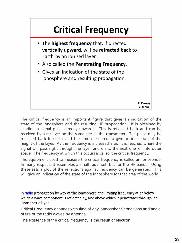
Critical Frequency• The highest frequency that, if directed
vertically upward, will be refracted back to Earth by an ionized layer.
• Also called the Penetrating Frequency.
• Gives an indication of the state of the ionosphere and resulting propagation.
Al Penney
VO1NO
The critical frequency is an important figure that gives an indication of the
state of the ionosphere and the resulting HF propagation. It is obtained by
sending a signal pulse directly upwards. This is reflected back and can be
received by a receiver on the same site as the transmitter. The pulse may be
reflected back to earth, and the time measured to give an indication of the
height of the layer. As the frequency is increased a point is reached where the
signal will pass right through the layer, and on to the next one, or into outer
space. The frequency at which this occurs is called the critical frequency.
The equipment used to measure the critical frequency is called an ionosonde.
In many respects it resembles a small radar set, but for the HF bands. Using
these sets a plot of the reflections against frequency can be generated. This
will give an indication of the state of the ionosphere for that area of the world
In radio propagation by way of the ionosphere, the limiting frequency at or below which a wave component is reflected by, and above which it penetrates through, an ionospheric layer.
Critical Frequency changes with time of day, atmospheric conditions and angle
of fire of the radio waves by antenna.
The existence of the critical frequency is the result of electron
39
limitation, i.e., the inadequacy of the existing number of free electrons to
support reflection at higher frequencies.
39

Critical Frequency
Critical Frequency and
below are reflected
back to Earth
Ionosphere
Frequencies > Critical
pass through Ionosphere
Al Penney
VO1NO
40

4000 km
• For E layer distances of 2000km, MUF = 5 x Critical Frequency
• For F layer distances of 4000km, MUF = 3 x Critical Frequency
Al Penney
VO1NO
The Critical Frequency can be used to calculate the MUF.

Lowest Usable Frequency
• Known as LUF.
• The lowest frequency at which communications are possible over a given path at a specified time 90% of the undisturbed days of the month.
• The amount of energy absorbed by the D layer directly impacts the LUF.
• Based on signal to noise ratio, so exact frequency depends on mode, power, antenna gain etc.
Al Penney
VO1NO
The lowest usable high frequency (LUF), in radio transmission, is
that frequency in the HF band at which the received field intensity is sufficient
to provide the required signal-to-noise ratio for a specified time period, e.g.,
0100 to 0200 UTC, on 90% of the undisturbed days of the month. The amount of energy absorbed by the lower regions of the ionosphere (D region, primarily)
directly impacts the LUF.
42

Al Penney
VO1NO
MUF/LUF taking into consideration the communication circuit (path from Belgium to Turkey with 100 W PEP). The propagation looks open on low bands with signals at night 40 dB stronger than at daytime.
43

Optimum Working Frequency
• A frequency approximately 15% less than the MUF that provides usable communications 90% of the time.
• Abbreviated FOT
Al Penney
VO1NO
Frequency of optimum transmission, in the transmission of radio waves via ionospheric reflection, is the highest effective (i.e. working) frequency that is predicted to be usable for a specified path and time for 90% of the days of the month. It is often abbreviated as FOT. The FOT is normally just below the value of the maximum usable frequency (MUF). In the prediction of usable frequencies, the FOT is commonly taken as 15% below the monthly median value of the MUF for the specified time and path.
The FOT is usually the most effective frequency for ionospheric reflection of radio waves between two specified points on Earth.
44

Solar Flux• A measure of radio energy emitted by the Sun.
• Considered to be one of the best ways to relate solar activity to propagation.
• Measured at 2800 MHz (bandwith 100 MHz) at the Dominion Radio Astrophysical Observatory in Penticton, BC.
• At solar min, SF = 50 to 60
• At solar max, SF = 200 or more
Al Penney
VO1NO
Emission from the Sun at centimetric (radio) wavelength is due primarily to coronal plasma trapped in the magnetic fields overlying active regions. The F10.7 index is a measure of the solar radio flux per unit frequency at a wavelength of 10.7 cm, near the peak of the observed solar radio emission. F10.7 is often expressed in SFU or solar flux units (1 SFU = 10-22 W m-2 Hz-1). It represents a measure of diffuse, nonradiative heating of the coronal plasma trapped by magnetic fields over active regions. It is an excellent indicator of overall solar activity levels and correlates well with solar UV emissions.
The solar F10.7 index is measured daily at local noon in a bandwidth of 100 MHz centered on 2800 MHz at the Penticton site of the Dominion Radio Astrophysical Observatory (DRAO), Canada. The solar F10.7 cm record extends back to 1947, and is the longest direct record of solar activity available, other than sunspot-related quantities.
Sunspot activity has a major effect on long distance radio communications particularly on the shortwave bands although medium wave and low VHF frequencies are also affected. High levels of sunspot activity lead to improved signal propagation on higher frequency bands, although they also increase the levels of solar noise and ionospheric disturbances. These effects are caused by impact of the increased level of solar radiation on the ionosphere.
45

Al Penney
VO1NO
The Dominion Radio Astrophysical Observatory is a research facility founded in 1960 and located south-west of Okanagan Falls, British Columbia, Canada. The site houses three instruments – an interferometric radio telescope, a 26-m single-dish antenna, and a solar flux monitor – and supports engineering laboratories. The DRAO is operated by the Herzberg Institute of Astrophysics of the National Research Council of the Canadian government.
46

Al Penney
VO1NO
Just what we need when propagation is poor!
47

International Space Environment Services

Fading• Variations in received signal strength.
• Some reasons for these variations in signal strength:
– Daily changes in ionosphere’s structure;
– Variations in shape/density of the ionosphere;
– Loss of signal due to multipath propagation; and
– Ionospheric disturbances.
Al Penney
VO1NO

Daily ChangesAl Penney
VO1NO
As the ionosphere changes over time, signals will fade or increase in strength. Example – European stations on 80M will gradually fade as the sun begins to rise in Europe and over the Atlantic. The increased ionization will cause the D layer to reconstitute, absorbing signals. On the other hand, as that is beginning, it will be time to look for stations towards the West. North Americans can start listening for Asia and Oceania before sunrise.
-Reduction in ionization levels near sunset.
-Increased absorption as D layer builds up.
-Differences in path length as ionization level changes in the refracting layer.
-Signals being reflected by different levels as ionization changes e.g.: E layer weakens and signal refracted off the F layer, meaning signal passes over the listener.

Shape/Density VariationsAl Penney
VO1NO
Random and time-varying differences in the shape and density of the ionosphere can result in fading as the signal path alternately increases and decreases in efficiency.

MultipathAl Penney
VO1NO
Selective fading or frequency selective fading is a radio
propagation anomaly caused by partial cancellation of a radio signal by itself —the signal arrives at the receiver by two different paths, and at least one of the
paths is changing (lengthening or shortening). This typically happens in the early evening or early morning as the various layers in the ionosphere move,
separate, and combine. The two paths can both be skywave or one
be groundwave.
Selective fading manifests as a slow, cyclic disturbance; the cancellation
effect, or "null", is deepest at one particular frequency, which changes constantly, sweeping through the received audio.
As the carrier frequency of a signal is varied, the magnitude of the change in
amplitude will vary. The coherence bandwidth measures the separation in
frequency after which two signals will experience uncorrelated fading.
•In flat fading, the coherence bandwidth of the channel is larger than the
bandwidth of the signal. Therefore, all frequency components of the signal will
experience the same magnitude of fading.
•In frequency-selective fading, the coherence bandwidth of the channel is
smaller than the bandwidth of the signal. Different frequency components of
the signal therefore experience uncorrelated fading.

•In general, the wider the signal bandwidth, the more susceptible it is to
selective fading.
52

Selective Fading• Signal cancels itself through Multipath.
• Can have different amount of phase changes/fading within the signal bandwidth.
• Gives AM voice signals a “hollow” sound.
• The narrower the signal bandwidth, the less susceptible it is.
Al Penney
VO1NO
Selective fading or frequency selective fading is a radio propagation
anomaly caused by partial cancellation of a radio signal by itself — the signal
arrives at the receiver by two different paths, and at least one of the paths is changing (lengthening or shortening).

Earth’s Geomagnetic Field
• The magnetic field that extends from the Earth's interior to where it meets the solar wind, a stream of charged particles emanating from the Sun.
• Interaction with charged particles in the solar wind can affect propagation.
Al Penney
VO1NO
Some of the charged particles from the solar wind are trapped in the Van Allen radiation belt. A smaller number of particles from the solar wind manage to travel, as though on an electromagnetic energy transmission line, to the Earth's upper atmosphere and ionosphere in the auroral zones. The only time the solar wind is observable on the Earth is when it is strong enough to produce phenomena such as the aurora and geomagnetic storms. Bright auroras strongly heat the ionosphere, causing its plasma to expand into the magnetosphere, increasing the size of the plasma geosphere, and causing escape of atmospheric matter into the solar wind. Geomagnetic storms result when the pressure of plasmas contained inside the magnetosphere is sufficiently large to inflate and thereby distort the geomagnetic field.
The solar wind is responsible for the overall shape of Earth's magnetosphere, and fluctuations in its speed, density, direction, and entrained magnetic field strongly affect Earth's local space environment. For example, the levels of ionizing radiation and radio interference can vary by factors of hundreds to thousands; and the shape and location of the magnetopause and bow shock wave upstream of it can change by several Earth radii, exposing geosynchronous satellites to the direct solar wind. These phenomena are collectively called space weather. The mechanism of atmospheric stripping is caused by gas being caught in bubbles of magnetic field, which are ripped off by solar winds. Variations in the magnetic field strength have been correlated to rainfall variation within the tropics.
54

Al Penney
VO1NO
55
Ionospheric Disturbances• Characterized by:
– Increased ionization in D Layer;
– Weakening or decomposition of F Layer; or
– Both.
Al Penney
VO1NO
56

Al Penney
VO1NO
A solar flare is a sudden flash of increased brightness on the Sun, usually
observed near its surface and in close proximity to a sunspot group. Powerful
flares are often, but not always, accompanied by a coronal mass ejection.
Even the most powerful flares are barely detectable in the total solar
irradiance (the "solar constant").
Solar flares occur in a power-law spectrum of magnitudes; an energy release
of typically 1020 joules of energy suffices to produce a clearly observable event,
while a major event can emit up to 1025 joules.
Flares are closely associated with the ejection of plasmas and particles
through the Sun's corona into outer space; flares also copiously emit radio
waves. If the ejection is in the direction of the Earth, particles associated with this disturbance can penetrate into the upper atmosphere (the ionosphere) and
cause bright auroras, and may even disrupt long range radio communication. It
usually takes days for the solar plasma ejecta to reach Earth. Flares also
occur on other stars, where the term stellar flare applies. High-energy
particles, which may be relativistic, can arrive almost simultaneously with the
electromagnetic radiations.
On July 23, 2012, a massive, potentially damaging, solar storm (solar flare,
coronal mass ejection and electromagnetic radiation) barely missed Earth. In
2014, Pete Riley of Predictive Science Inc. published a paper in which he attempted to calculate the odds of a similar solar storm hitting Earth within the

next 10 years, by extrapolating records of past solar storms from the 1960s to
the present day. He concluded that there may be as much as a 12% chance of
such an event occurring.
57

58

Al Penney
VO1NO
Solar flares strongly influence the local space weather in the vicinity of the
Earth. They can produce streams of highly energetic particles in the solar
wind or stellar wind, known as a solar proton event. These particles can impact
the Earth's magnetosphere, and present radiation hazards to spacecraft and
astronauts. Additionally, massive solar flares are sometimes accompanied by coronal mass ejections (CMEs) which can trigger geomagnetic
storms that have been known to disable satellites and knock out terrestrial
electric power grids for extended periods of time.
The soft X-ray flux of X class flares increases the ionization of the upper
atmosphere, which can interfere with short-wave radio communication and can
heat the outer atmosphere and thus increase the drag on low orbiting
satellites, leading to orbital decay. Energetic particles in the magnetosphere contribute to the aurora borealis and aurora australis. Energy in the form of
hard x-rays can be damaging to spacecraft electronics and are generally the
result of large plasma ejection in the upper chromosphere.
The radiation risks posed by solar flares are a major concern in discussions of a manned mission to Mars, the Moon, or other planets. Energetic protons can
pass through the human body, causing biochemical damage, presenting a
hazard to astronauts during interplanetary travel. Some kind of physical or
magnetic shielding would be required to protect the astronauts. Most proton storms take at least two hours from the time of visual detection to reach

Earth's orbit. A solar flare on January 20, 2005 released the highest concentration of protons ever directly measured, giving astronauts as little as
15 minutes to reach shelter.
59

Ionospheric Disturbances
Al Penney
VO1NO
60
Al Penney
VO1NO
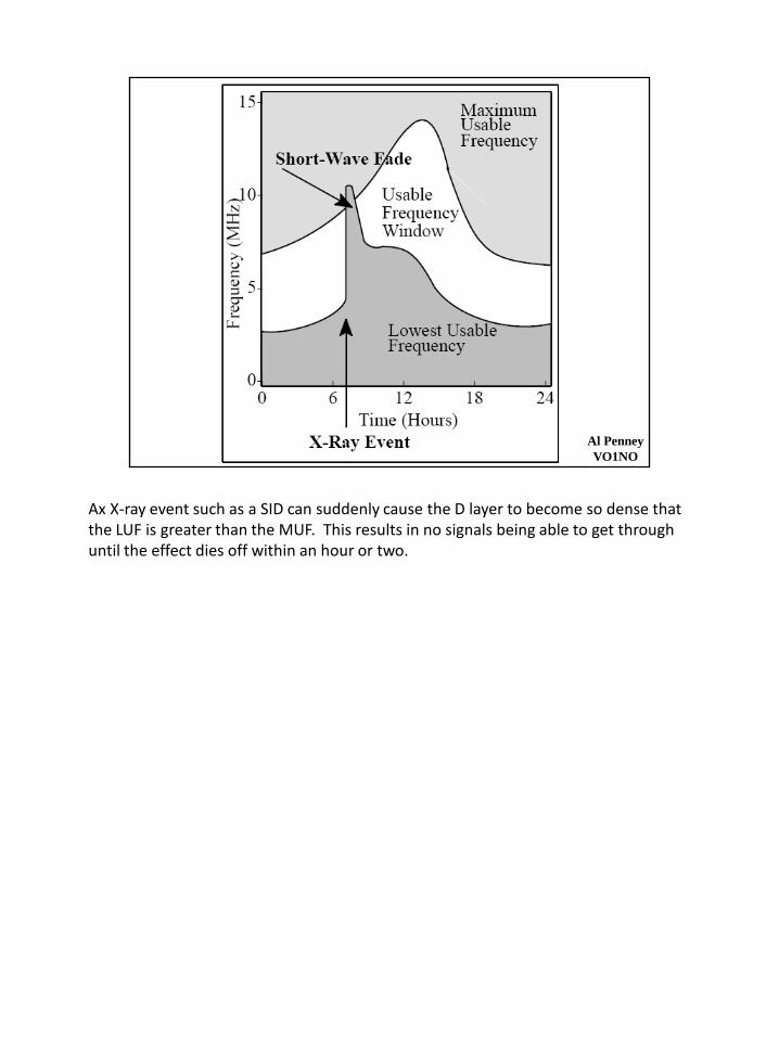
Ax X-ray event such as a SID can suddenly cause the D layer to become so dense that the LUF is greater than the MUF. This results in no signals being able to get through until the effect dies off within an hour or two.

K Index• Quantifies disturbances in Earth’s magnetic field.
• Quasi-logarithmic scale 0 to 9
• 1 = calm
• 5 or higher = geomagnetic storm
• Updated every 3 hours (8 measurements per day)
• Planet’s K Index (Kp) is average of all observatories’ K Index around the world.
Al Penney
VO1NO
The K-index quantifies disturbances in the horizontal component of earth's magnetic field with an integer in the range 0-9 with 1 being calm and 5 or more indicating a geomagnetic storm. It is derived from the maximum fluctuations of horizontal components observed on a magnetometer during a three-hour interval. The label 'K' comes from the German word 'Kennziffer' meaning 'characteristic digit.‘ The K-index was introduced by Julius Bartels in 1938.
There are two indices that are used to determine the level of geomagnetic acitivity: the A index and the
K index. These give indications of the severity of the magnetic fluctuations and hence the dis-turbance to the ionosphere. The first of the two indices used to measure geomagnetic activity is the K index. Each magnetic observatory calibrates its magnetometer so that its K index describes the same level of magnetic disturbance, no matter whether the observatory is located in the auroral regions or at the Earth’s equator. At three hourly intervals starting at 0000 UTC each day, the maximum deviations from the quiet day curve at a particular observatory are determined and the largest value is selected. This value is then manipulated mathematically and the K index is calculated for that location
The K-scale is quasi-logarithmic. The conversion table from maximum fluctuation R (nT) to K-index, varies from observatory to observatory in such a way that the historical rate of occurrence of certain levels of K are about the same at all observatories. In practice this means that observatories at higher geomagnetic latitude require higher levels of fluctuation for a given K-index. For example, at Godhaven, Greenland, a value of K equal to 9 is derived with R=1500 nT, while in Honolulu, HI, a fluctuation of only 300 nT is recorded as K=9. In Kiel, Germany, K=9 corresponds to R=500 nT or greater.[3] The real-time K-index is determined
62

after the end of prescribed three-hour intervals (0000-0300, 0300-0600, ..., 2100-2400). The maximum positive and negative deviations during the 3-hour period are added together to determine the total maximum fluctuation. These maximum deviations may occur any time during the 3-hour period.
The Kp index and estimated Kp index
The official planetary Kp index is derived by calculating a weighted average of K-indices from a network of geomagnetic observatories. Since these observatories do not report their data in real-time, various operations centers around the globe estimate the index based on data available from their local network of observatories. The Kp-index was introduced by Bartels in 1949.[1]
The Kp index is used for the study and prediction of ionospheric propagation of high frequency radio signals. Geomagnetic storms, indicated by a Kp of 5 or higher, have no direct effect on propagation. However they disturb the F-layer of the ionosphere, especially at middle and high geographical latitudes, causing a so-called ionospheric storm which degrades radio propagation. The degradation mainly consists of a reduction of the maximum usable frequency (MUF) by as much as 50%.[6] Sometimes the E-layer may be affected as well. In contrast with sudden ionospheric disturbances (SID), which affect high frequency radio paths near the Equator, the effects of ionospheric storms are more intense in the polar regions
62

A Index• Measure of daily level of geomagnetic activity.
• Values of 8 daily K indices at observatories around the world are used to calculate daily A Index for each observatory.
• Can range in value from 0 to 400 or so.
• 0 = very calm, while 400 = Very major magnetic storm!
• Planet’s overall A Index (Ap) is average of A indices for all observatories around the world.
Al Penney
VO1NO
The A-index provides a daily average level for geomagnetic activity. Because of the non-linear relationship of the K-scale to magnetometer fluctuations, it is not meaningful to take averages of a set of K indices. What is done instead is to convert each K back into a linear scale called the "equivalent three hourly range" a-index (note the lower case).
The K index is a “quasi logarithmic” number and as such cannot be averaged to give a longer-term view of the state of the Earth’s magnetic field. Thus was born the A index, a daily average. At each 3-hour increment the K index at an observatory is converted to an equivalent “a”
index using a Table, and the 8 a-index values are averaged to produce the A index for that day. It can vary up to values around 100. During very severe geomagnetic storms it can reach values of up to 200 and very occasionally more. The A index reading varies from one observatory to the next, since magnetic disturbances can be local. To overcome this, the indices are averaged over the globe to provide the Ap index, the planetary value
A Index
The A index is a linear measure of the Earth's field. As a result of this, its values extend over amuch wider range. It is derived from the K index by scaling it to give a linear value which istermed the "a" index. This is then averaged over the period of a day to give the A index. Likethe K index, values are averaged around the globe to give the planetary Ap index.
Values for the A index range up to 100 during a storm and may rise as far as 400 in a severegeomagnetic storm.
A index & Kp index relationship
Although the A index and K index are different values it is possible to relate these indicestogether. A summary of this relationship is given int he table below.
RELATIONSHIP BETWEEN KP INDEX AND A INDEX
AP INDEX
KP INDEX
DESCRIPTION
63

0
0
Quiet
4
1
Quiet
7
2
Unsettled
15
3
Unsettled
27
4
Active
48
5
Minor storm
80
6
Major storm
132
7
Severe storm
208
8
Very major storm
400
9
Very major storm
63

NVIS Propagation• Near Vertical Incidence Skywave
• Skywave propagation 0 – 650 km.
• Signals travel vertically or near verticallybefore being refracted back to Earth.
• Used on 160, 80, 60 and 40M bands.
• Suitable for emergency communications, regional communications and mountainous regions.
Al Penney
VO1NO
Near vertical incidence skywave, or NVIS, is a skywave radio-wave
propagation path that provides usable signals in the distances range —usually 0–650 km (0–400 miles). It is used for military
and paramilitary communications, broadcasting, especially in the
tropics, and by radio amateurs for nearby contacts circumventing line-
of-sight barriers. The radio waves travel near-vertically upwards into the ionosphere, where they are refracted back down and can be
received within a circular region up to 650 km (400 miles) from the transmitter. If the frequency is too high (that is, above the critical
frequency of the ionospheric F layer), refraction fails to occur and if it is
too low, absorption in the ionospheric D layer may reduce the signal
strength.
There is no fundamental difference between NVIS and conventional
skywave propagation; the practical distinction arises solely from
different desirable radiation patterns of the antennas (near vertical for
NVIS, near horizontal for conventional long-range skywave
propagation).

NVIS Propagation
Al Penney
VO1NO
Near vertical incidence skywave, or NVIS, is a skywave radio-wave
propagation path that provides usable signals in the distances range —usually 0–650 km (0–400 miles). It is used for military
and paramilitary communications, broadcasting, especially in the
tropics, and by radio amateurs for nearby contacts circumventing line-
of-sight barriers. The radio waves travel near-vertically upwards into the ionosphere, where they are refracted back down and can be
received within a circular region up to 650 km (400 miles) from the transmitter. If the frequency is too high (that is, above the critical
frequency of the ionospheric F layer), refraction fails to occur and if it is
too low, absorption in the ionospheric D layer may reduce the signal
strength.
There is no fundamental difference between NVIS and conventional
skywave propagation; the practical distinction arises solely from
different desirable radiation patterns of the antennas (near vertical for
NVIS, near horizontal for conventional long-range skywave
propagation).
The most reliable frequencies for NVIS communications are between 1.8 MHz and 8 MHz. Above 8 MHz, the probability of success begins to
decrease, dropping to near zero at 30 MHz. Usable frequencies are
dictated by local ionospheric conditions, which have a strong systematic
dependence on geographical location. Common bands used in amateur radio at mid-latitudes are 3.5 MHz at night and 7 MHz during daylight, with
experimental use of 5 MHz (60 meters) frequencies. During winter nights at the
bottom of the sunspot cycle, the 1.8 MHz band may be required. Broadcasting
uses the tropical broadcast bands between 2.3 and 5.06 MHz, and
the international broadcast bands between 3.9 and 6.2 MHz. Military NVIS
communications mostly take place on 2–4 MHz at night and on 5–7 MHz
during daylight.
Optimum NVIS frequencies tend to be higher towards the tropics and lower
towards the arctic regions. They are also higher during high sunspot activity
years. The usable frequencies change from day to night, because sunlight causes the lowest layer of the ionosphere, called the D layer, to increase,
causing attenuation of low frequencies during the day while the maximum
usable frequency (MUF) which is the critical frequency of the F layer rises with
greater sunlight. Real time maps of the critical frequency are available. Use
of a frequency about 15% below the critical frequency should provide reliable NVIS service. This is sometimes referred to as the optimum working
frequency or FOT.
NVIS is most useful in mountainous areas where line-of-sight propagation is
ineffective, or when the communication distance is beyond the 50 mile (80 km)
range of groundwave (or the terrain is so rugged and barren that groundwave
is not effective), and less than the 300–1500 mile (500–2500 km) range of
lower-angle sky-wave propagation. Another interesting aspect of NVIS
communication is that direction finding of the sender is more difficult than for
ground-wave communication (i.e. VHF or UHF). For broadcasters, NVIS
allows coverage of an entire medium-sized country at much lower cost than with VHF (FM), and daytime coverage, similar to mediumwave (AM
broadcast) nighttime coverage at lower cost and often with less interference.
65

NVIS Frequency• Generally in the range 1.8 – 8 MHz.
• Must be less than Critical Frequency of F2 layer.
• Main criteria is local ionospheric conditions:– D-layer absorption attenuates low frequencies during day;
– F2 Critical Frequency higher during day, lower at night;
– Optimum frequencies higher in tropics, lower in Arctic; and
– Optimum frequencies lower during solar minimum.
• Will usually need daytime and nighttime frequencies.
• Optimum frequency generally 10-15% below F2 Critical Frequency (foF2).
Al Penney
VO1NO
The selection of an appropiated working frequency is essential for a successful operation in NVIS. As a general rule, we will choose a
frequency 10% to 15% below the ionosphere's F2 layer critical frequency (foF2) at a given time.
It is of particular importance not to confuse the foF2 with the MUF. The critical frequency foF2 is the maximum frequency that a radio wave can have in order to be reflected in the F2 layer when arriving at this layer with an angle of incidence of 90 degrees (perpendicular). In the MUF, angles of incidence different of 90 degrees are considered, which practically means that a different MUF will exist for each distance of a HF radio link.
Our goal now is to get foF2 forecasts or, much better, real time measurements of the foF2 made with an ionosonde nearby our transmitter station at a close time. Let's not forget that the foF2 has significant changes over the day and also that it will be different depending on the transmitter location.
In order to get this data, we can check the web site of the Mass Lowel University Center for Atmospheric Research (Massachussetts, USA), where there is a record of foF2 values (among other parameters) measured by ionosondes all around the world.

http://ulcar.uml.edu/stationmap.html
Near vertical incidence skywave, or NVIS, is a skywave radio-wave
propagation path that provides usable signals in the distances range — usually
0–650 km (0–400 miles). It is used for military
and paramilitary communications, broadcasting, especially in the tropics, and
by radio amateurs for nearby contacts circumventing line-of-sight barriers. The
radio waves travel near-vertically upwards into the ionosphere, where they
are refracted back down and can be received within a circular region up to 650
km (400 miles) from the transmitter. If the frequency is too high (that is, above
the critical frequency of the ionospheric F layer), refraction fails to occur and if
it is too low, absorption in the ionospheric D layer may reduce the signal
strength.
There is no fundamental difference between NVIS and conventional skywave
propagation; the practical distinction arises solely from different desirable
radiation patterns of the antennas (near vertical for NVIS, near horizontal for
conventional long-range skywave propagation).
The most reliable frequencies for NVIS communications are between 1.8 MHz
and 8 MHz. Above 8 MHz, the probability of success begins to decrease,
dropping to near zero at 30 MHz. Usable frequencies are dictated by local
ionospheric conditions, which have a strong systematic dependence on
geographical location. Common bands used in amateur radio at mid-latitudes are 3.5 MHz at night and 7 MHz during daylight, with experimental use of
5 MHz (60 meters) frequencies. During winter nights at the bottom of the
sunspot cycle, the 1.8 MHz band may be required. Broadcasting uses
the tropical broadcast bands between 2.3 and 5.06 MHz, and the international
broadcast bands between 3.9 and 6.2 MHz. Military NVIS communications
mostly take place on 2–4 MHz at night and on 5–7 MHz during daylight.
Optimum NVIS frequencies tend to be higher towards the tropics and lower
towards the arctic regions. They are also higher during high sunspot activity
years. The usable frequencies change from day to night, because sunlight causes the lowest layer of the ionosphere, called the D layer, to increase,
causing attenuation of low frequencies during the day while the maximum
usable frequency (MUF) which is the critical frequency of the F layer rises with
greater sunlight. Real time maps of the critical frequency are available. Use
of a frequency about 15% below the critical frequency should provide reliable NVIS service. This is sometimes referred to as the optimum working
frequency or FOT.
66

NVIS is most useful in mountainous areas where line-of-sight propagation is
ineffective, or when the communication distance is beyond the 50 mile (80 km)
range of groundwave (or the terrain is so rugged and barren that groundwave
is not effective), and less than the 300–1500 mile (500–2500 km) range of
lower-angle sky-wave propagation. Another interesting aspect of NVIS
communication is that direction finding of the sender is more difficult than for
ground-wave communication (i.e. VHF or UHF). For broadcasters, NVIS
allows coverage of an entire medium-sized country at much lower cost than with VHF (FM), and daytime coverage, similar to mediumwave (AM
broadcast) nighttime coverage at lower cost and often with less interference.
66

F2 Critical Frequency foF2
• Measured with Ionosondes or Chirpsounders:
– Upward pointing radar sweeps through 1.6 – 12 MHz;
– Echos indicate height of ionosphere reflecting layers;
– Results displayed on an Ionogram.
• Measurements taken throughout world:
An ionosonde, or chirpsounder, is a special radar for the examination of
the ionosphere. The basic ionosonde technology was invented in 1925
by Gregory Breit and Merle A. Tuve [1] and further developed in the late 1920s
by a number of prominent physicists, including Edward Victor Appleton. The
term ionosphere and hence, the etymology of its derivatives, was proposed
by Robert Watson-Watt.
An ionosonde consists of:
•A high frequency (HF) radio transmitter, automatically tunable over a wide
range. Typically the frequency coverage is 0.5–23 MHz or 1–40 MHz, though
normally sweeps are confined to approximately 1.6–12 MHz.
•A tracking HF receiver which can automatically track the frequency of the
transmitter.
•An antenna with a suitable radiation pattern, which transmits well vertically
upwards and is efficient over the whole frequency range used.
•Digital control and data analysis circuits.
The transmitter sweeps all or part of the HF frequency range, transmitting
short pulses. These pulses are reflected at various layers of the ionosphere, at heights of 100–400 km, and their echos are received by the receiver and
analyzed by the control system. The result is displayed in the form of an ionogram, a graph of reflection height (actually time between transmission

and reception of pulse) versus carrier frequency.
An ionosonde is used for finding the optimum operation frequencies for
broadcasts or two-way communications in the high frequency range.
67

Ionogram
•Digisonde ionogram presents signals reflected from the ionosphere in the
frequency vs travel time frame, with signal strength indicated by the pixel
intensity, and wave polarization, angle of arrival, and Doppler frequency
indicated by colors
•Individual reflected signals (echoes) observed on each sounding frequency
form traces in the ionogram image
•Red (green) colors indicate vertical echoes with O-polarization (X-polarization)
•ARTIST software scales the ionogram and calculates the vertical Electron
Density Profile (EDP) in real time
•Thin black lines show the ARTIST-identified O-traces
•The black line with uncertainty bars shows the calculated bottomside EDP
•Extraction and interpretation of the signal traces in ionogram images is an
intelligent, machine-hard problem of feature recognition
Extraordinary Frequency - As a wave approaches the reflection point, its group velocity approaches zero and this increases the time-of-flight of the signal. Eventually, a frequency is reached that enables the wave to penetrate the layer without being reflected. For ordinary mode waves, this occurs when the transmitted frequency

just exceeds the peak plasma frequency of the layer. In the case of the extraordinary wave, the magnetic field has an additional effect, and reflection occurs at a frequency that is higher than the ordinary wave by half the electron gyrofrequency.
In order to gain a view of the state of the ionosphere for various forms of radio
communication, a test instrument known as an ionosonde is used.
The test instrument is sometimes also known as a vertical incidence sounder,
VIS, and this name gives an indication of the operation of the ionosonde.
Ionosondes, and the ionograms they produce are essential test instruments
used for investigating the state of the ionosphere. The outputs they produce
are able to give an indication of the state of the ionosphere above them that
can be used to create a picture of what the ionospheric conditions are like at
that moment.
By detecting the state of the ionosphere using an ionosonde it is possible to
build up a picture of the actual state of the ionosphere at that moment and
also at that point on the globe. Using a network of these test instruments
around the globe a more accurate picture can be built up and this data can be
used to determine the optimum frequencies for HF broadcasting and radio
communication links, both short range and long distance radio
communication.
The concept of the ionosonde is that it is a form of test instrument that
transmits pulses of RF power vertically upwards. It then receives the signal that
is reflected and this shows many details about the ionosphere above it.
The signal is directed upwards towards the ionosphere. The signal rises and at
some point it is possible that it is reflected back to Earth and received by a
receiving antenna and system.
The signal is normally pulsed, like that of a conventional radar, and using the
time delay for the returned signal, it is possible to determine the height of
reflection.
Accordingly, it can be seen that the ionosonde is effectively a specialised form
of pulsed radar that is used to detect the ionisation in the ionosphere.
The plot of the ionosonde output is called an ionograph and in early days this
would have been printed out on paper, but modern systems will obviously use
computer technology, storing the data for processing and display as required.
The signal from the ionosonde starts at a low frequency and is stepped up infrequency. Initially the signal is reflected back by the ionosphere, but as the
68

frequency is increased it penetrates deeper into the relevant region and
eventually passes on to the next ionised region where the same process occurs
as the frequency is swept upwards. Eventually a point is reached where the
signal passes though all the regions of the ionosphere and it is not reflected.
There is a time delay between when the signal is transmitted and the reflected
signal is received. Knowing the speed that the signals travel, it is possible to
convert this into a distance or height figure.
There is a variety of instruments that have been used over the years from
different manufacturers and with different specifications but in essence they all
provide the same function.
There have been many developments in ionosonde technology. Analogue
systems were used up until the 1970s. These systems all swept through the
relevant parts of the spectrum, normally from about 1 MHz up to between 15
and 25 MHz.
They generally used a relatively high power level, often up to 25 kW. Sweeps
could take anywhere between about 30 seconds and 2 minutes which gave
them the ability to look at relatively short term variations in the ionosphere.
Since the 1970s digital systems have been used. These provide essentially the
same as the analogue ones, but provide considerably more facilities and they
are able to manipulate the data far more easily as they use computing and
digital signal processing technology.
What is an Ionogram
An ionogram is the form of plot that is produced by an ionosonde. It is
essentially a plot of the altitude against frequency.
The vertical axis shows the height and the horizontal axis shows the frequency.
From the ionogram it is possible to see the critical frequencies for each of theionospheric regions or layers. These are labelled as f0 for each layer or region.
In other words f0 E is the critical frequency for the E region, etc.
From the diagram, it can be seen that the signal is sent upwards and initially it
is absorbed by the D layer and no reflection is seen.
As the signal moves up in frequency, it starts to be reflected back to the
ground by the E region and the delay in receiving the pulse enables the
approximate height to be determined.
As the frequency increases, the height of the reflection increases as the signal
penetrates further into the E region. Ultimately the rate at which the signal
penetrates the region for a given increase in frequency increases as the signal
reaches the point at which it passes through the region. The actual frequencyat which it passes through the E region is called the critical frequency, f0 E.
68

Above f0 E, the signal reaches the F1 region (assuming the F region has split
into two) and the process repeats. Again the same process repeats for the F2,
until the signal passes through all the different regions and travels on into
outer space.
In reality the actual ionograms are less distinct than the diagrammatic ones,
but the same basic patters can be made out.
68

Optimum NVIS Frequency
• On previous page, foF2 = 4.838 MHz.
• Optimum NVIS frequency is foF2 – 10 to 15%:4.838 – 10% = 4.354 MHz
4.838 – 15% = 4.112 MHz
• Therefore, Optimum NVIS frequency range at that location and time is 4.112 to 4.354 MHz.
• Amateurs can use 80M band, Military can select a frequency closest to that range, but always belowCritical Frequency foF2.
• Remember – you may need day/night frequencies.
An ionogram is a display of the data produced by an ionosonde. It is a graph
of the virtual height of the ionosphere plotted against frequency. Ionograms
are often converted into electron density profiles. Data from ionograms may be used to measure changes in the Earth's ionosphere due to space
weather events.
Chirp transmitter
A chirp transmitter is a shortwave radio transmitter that sweeps the HF radio
spectrum on a regular schedule. If one is monitoring a specific frequency, then
a chirp is heard (in CW or SSB mode) when the signal passes through. In
addition to their use in probing ionospheric properties, these transmitters are
also used for over-the-horizon radar systems.

Ionosonde Data
• Canadian data available at (account required):
– http://chain.physics.unb.ca/chain/pages/rules
• Other data at Global Ionosphere Radio Observatory:
– http://giro.uml.edu/ionogram-data.html
– Select closest location: https://ulcar.uml.edu/stationlist.htmlhttp://giro.uml.edu/IonogramMovies/
– One Canadian location – Argentia
– Millstone Hill, Massachussetts may be closest for Ontario
The Canadian High Arctic Ionospheric Network (CHAIN) is an array of
ground-based radio instruments deployed in the Canadian Arctic and operated
by the University of New Brunswick. The CHAIN instruments include high data-
rate GPS receivers and digital ionosondes. After passing through the
Earth's ionosphere, microwave GPS signals carry information about the total
electron content (TEC). This information is commonly used to improve the
precision of GPS and to study ionospheric morphology. Ionosondes transmit
pulses of radio signals in the Medium Frequency (MF) and High
Frequency (HF) ranges, whose echos are analyzed to measure height and
density of the ionosphere. Advanced digital ionosondes used in the CHAIN
network are also able to measure the bulk motion of ionospheric plasma.
Most of the CHAIN instruments are located within the polar cap defined as a region of open magnetic field lines. The polar cap ionosphere is directly linked
to the interplanetary magnetic field carried by the solar wind. Polar cap thus
provides a vantage point for the study of energy exchange between the solar
wind, magnetosphere and ionosphere.
CHAIN is an integral part of the Canadian Geospace Monitoring (CGSM)
programme. It provides ground support for Canadian and international scientific space missions such as THEMIS and CASSIOPE.
In January 2012, the Canada Foundation for Innovation announced funding for the Expanded Canadian High-Arctic Ionospheric Network (ECHAIN). This
funding was used to add 15 Global Positioning System (GPS) receivers to the
existing network of GPS receivers and radars of the Canadian High Arctic
Ionospheric Network (CHAIN). The data will contribute significantly to the
progress of space research by providing a better understanding of the
processes in the Sun-Earth system.
70
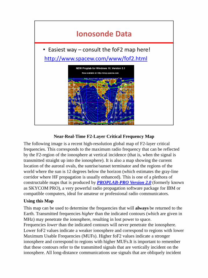
Ionosonde Data
• Easiest way – consult the foF2 map here!
http://www.spacew.com/www/fof2.html
Near-Real-Time F2-Layer Critical Frequency Map
The following image is a recent high-resolution global map of F2-layer critical
frequencies. This corresponds to the maximum radio frequency that can be reflected
by the F2-region of the ionosphere at vertical incidence (that is, when the signal is
transmitted straight up into the ionosphere). It is also a map showing the current
location of the auroral ovals, the sunrise/sunset terminator and the regions of the
world where the sun is 12 degrees below the horizon (which estimates the gray-line
corridor where HF propagation is usually enhanced). This is one of a plethora of
constructable maps that is produced by PROPLAB-PRO Version 2.0 (formerly known
as SKYCOM PRO), a very powerful radio propagation software package for IBM or
compatible computers, ideal for amateur or professional radio communicators.
Using this Map
This map can be used to determine the frequencies that will always be returned to the
Earth. Transmitted frequencies higher than the indicated contours (which are given in
MHz) may penetrate the ionosphere, resulting in lost power to space.
Frequencies lower than the indicated contours will never penetrate the ionosphere.
Lower foF2 values indicate a weaker ionosphere and correspond to regions with lower
Maximum Usable Frequencies (MUFs). Higher foF2 values indicate a stronger
ionosphere and correspond to regions with higher MUFs.It is important to remember
that these contours refer to the transmitted signals that are vertically incident on the
ionosphere. All long-distance communications use signals that are obliquely incident

on the ionosphere (that is, the radio signals are passing through the ionosphere at an
angle instead of head-on).
The purpose of this map is to help illustrate regions of the ionosphere that are weak
and strong. Critical F2 layer frequencies in excess of about 8 MHz correspond to
regions of the ionosphere that are relatively strong and capable of reflecting high-
frequency signals over longer distances. Critical frequencies below about 4 MHz are
weaker and will result in greater signal loss to space, lower MUFs and greater signal
instability.
The map shows the radio auroral zones as green bands near the northern and southern
poles. The area within the green bands is known as the auroral zone. Radio signals
passing through these auroral zones will experience increased signal degradation in
the form of fading, multipathing and absorption.
The radio auroral zones are typically displaced equatorward from the optical auroral
zones (or the regions where visible auroral activity can be seen with the eye).
The great-circle signal path from the Eastern United States to Tokyo is shown along
with the distance of the path (in km) and the bearing from the U.S. to Tokyo (in
degrees from north).
If this signal path crosses through the green lines indicating the position and width of
the radio auroral zones, propagation will be less stable and degraded compared to if
the signal never crossed through the auroral zones. Using your mouse, PROPLAB-
PRO will let you plot the great-circle paths and azimuths between any two
points while this display is continually updated.
The yellow Sun symbol near the equator indicates the location where the Sun is
directly overhead. The regions of the world where the Sun is exactly rising or
setting is known as the Grayline and is shown as the solid gray-colored line that is
closest to the Sun symbol. The second solid gray-colored line defines the regions of
the world where the Sun is exactly 12 degrees below the horizon. This line defines the
end of evening twilight. Everything inside of this second line is experiencing night-
time conditions. The area between the two lines (shaded a lighter shade than the night-
time sector) is known as the grayline and has special significance to radio
communicators. Signals which travel inside the grayline region often experience
significant improvements in propagation because of the loss of ionization in the D-
region as the Sun sets. However, because the higher F-regions of the ionosphere
remain strongly ionized for longer periods of time, signals with higher frequencies are
able to travel to greater distances with less attenuation when they are within the
grayline. The great-circle path from the eastern U.S. to Japan is also shown with the
accompanying distance (in kilometers) and bearing (clockwise from north). Notice
how this path may occassionally pass into the influential auroral zones if geomagnetic
activity increases or during the night-times.
71

NVIS Antenna Pattern
Al Penney
VO1NO
We’ll look at NVIS antennas in more detail in Ch 8.

Greyline Propagation• Greyline or Terminator is line that separates
sunlight from darkness around Earth.
• Enhanced propagation along Greyline (sunrise and sunset).
• D layer disappears,
but F layer still there.
• Used primarily on low
bands (160M and 80M).
Grey line or gray line propagation is a form of radio signal propagation that
provides surprisingly long distance radio communications at dawn and dusk
sometimes when other forms of ionospheric propagation may not be expected
to provide signal paths of these distances.
Grey line propagation is only present around dawn and dusk and therefore it
cannot be used to support global radio communications at any time.
Accordingly it tends to be used chiefly by radio amateurs and a few other users
who can accommodate the timing and other limitations of its availability.
For grey line propagation signals travel along the grey or twilight zone
between night and day. This is area where night and day meet and it is also
known as the terminator. In this region signals on some frequencies are
attenuated much less than might normally be experienced and as a result
signals can be received at surprisingly high levels over very long distances -
even from the other side of the globe.
The improved propagation conditions around the grey line are most noticeable
primarily on the lower frequency bands in the HF portion of the spectrum
where the level of ionisation in the D layer has a much greater effect on signals
that on those frequencies higher up.
The diagram below shows how the illumination remains on the F region much
longer than on the D region, and this creates a situation where the D region

has faded away, but the F region remains intact.
In reality, the D region fades before dusk as the illumination from the sun
reduces around dusk at the Earths surface. The level of ionisation in the D
region drops very quickly around dusk and after dark because the air density is
high and recombination of the free electrons and positive ions occurs
comparatively quickly.
This occurs while the level of ionisation is still high within the F layer, which
gives most of the radio propagation for long distance radio communications.
This occurs because the F region is much higher in altitude, and as the Sun sets
it remains illuminated by the Sun's radiation for longer than the D region,
which is lower down. Also recombination of the ions takes longer because the
air is very much thinner at the altitude of the F region compared to that of the
D region.
The same occurs in the morning as the Sun rises. The F region receives
radiation from the Sun before the D region and its ionisation level starts to rise
before that of the D region. As the level of the D region ionisation is low, this
means that the degree of attenuation to which the lower frequency signals are
subjected to is very much less than in the day. This also occurs at a time when
the F region ionisation is still very high, and good reflections are still
achievable. Accordingly this results in much lower overall path losses around the grey line than are normally seen.
In fact, when looking at the region of the radio terminator it should be
remembered that there are a variety of variables that mean that it does not
exactly follow the day time / night time terminator as seen on the Earth's
surface. The ionised regions are well above the Earth's surface and are
accordingly illuminated for longer, although against this the Sun is low in the
sky and the level of ionisation is low. Furthermore there is a finite time required
for the level of ionisation to rise and decay. As there are many variables
associated with the "radio signal propagation" terminator, the ordinary
terminator should only be taken as a rough guide for radio signal propagation
conditions.
Although it may be obvious to mention, grey line propagation can only exist
for stations at locations that fall along the grey line or terminator. This
significantly limits the number of areas for a given station at a particular
location to set up long distance communication, although there will be slight
changes over the course of the year for many stations.
73

Frequencies that are affected by this form of propagation are generally limited
to frequencies up to about 10 MHz. Frequencies higher in frequency than 10
MHz tend to be attenuated to only a minor degree by the D region and
therefore there is little or no enhancement around dusk and dawn by this
mechanism.
Grey line propagation is particularly noticeable on lower frequencies, for
example the 3.5 MHz amateur radio band. Normally signals may be heard over
distances of a few hundred kilometres in the day, and possibly up to or two
thousand kilometres at night for those stations with good antennas.
Grey line propagation regularly enables long distance radio communication
contacts to be made with stations the other side of the globe at very good
strength levels.
The optimum times are normally around the spring and autumn equinoxes as
neither end of the link is subject to the propagation extremes of summer and
winter. It is at these times of year that long distance radio communication can
be established with stations onth e other side of the globe at remarkably good
signal strength levels.
Grey line enhancements over the course of the year
The path of the grey line changes during the course of the year. As the angle
subtended by the Sun's rays changes with the seasons, so the line taken by the
terminator changes. This results from the fact that during the winter months,
the Northern Hemisphere of the earth is titled away from the Sun, and towards
it during the summer months.
The converse is obviously true for the southern hemisphere. In addition to this
the width of the grey line also changes. It is much wider towards the poles
because the line between dark and light is less will defined as a result of the
fact that the Sun never rises high in the sky at the poles. It is also much
narrower at the equator. This results in grey line propagation being active for
longer at the poles than at the equator.
Grey line propagation provides an opportunity for long distance radio
communication contacts and links to be made, often with stations the other
side of the globe. Signals travel along the grey line, or terminator and suffer
comparatively little attenuation. An opening via grey line propagation may only
last for half an hour, but it gives the opportunity for radio communication to
be established between stations as far away as the other side of the globe.
The gray line, sometimes called the twilight zone, is a band around the Earth between
73

the sunlit portion and
darkness. Astronomers call this the terminator. The terminator is a somewhat diffused
region because the Earth’s
atmosphere tends to scatter the light into the darkness. Fig 34 illustrates the gray line.
Notice that on one side of
the Earth, the gray line is coming into daylight (sunrise), and on the other side it is
coming into darkness (sunset).
Propagation along the gray line is very efficient, so greater distances can be covered
than might be
expected for the frequency in use. One major reason for this is that the D layer, which
absorbs HF signals,
disappears rapidly on the sunset side of the gray line, and has not yet built up on the
sunrise side.
The gray line runs generally north and south, but varies as much as 23 either side of
the north-south
line. This variation is caused by the tilt of the Earth’s axis relative to its orbital plane
around the Sun. The
gray line will be exactly north and south at the equinoxes (March 21 and September
21). On the first day of
Northern Hemisphere summer, June 21, it is tilted to the maximum of 23 one way,
and on December 21,
the first day of winter, it is tilted 23 the other way.
To an observer on the Earth, the direction of the terminator is always at right angles to
the direction of the
Sun at sunrise or sunset. It is important to note that, except at the equinoxes, the gray-
line direction will be
different at sunrise from that at sunset. This means you can work different areas of the
world in the evening
than you worked in the morning.
It isn’t necessary to be located inside the twilight
zone in order to take advantage of gray-line
propagation. The effects can be used to advantage
before sunrise and after sunset. This is because the
Sun “rises” earlier and “sets” later on the ionospheric
layers than it does on the Earth below.
73

Greyline Propagation• Position of greyline changes throughout year
because of 23 degree tilt of Earth’s axis.
• Also changes dawn to dusk of same day.
74

Propagation – 630M• 472 – 479 kHz
• Relatively new Amateur band – low activity
• Both Surface Wave and Sky Wave propagation
• Surface Wave very reliable out to several hundred km
• Sky Wave at night, especially when solar cycle is at a low point
• Several thousand km possible via Sky Wave
• Sky Wave uses mostly E Layer, not F layer
Propagation on the 630m band is different in many respects from that in the HF
spectrum. Because propagation will have an impact on how the band will be used, a
quick description is in order.
Propagation at MF wavelengths is via both ground waves and skywaves. Ground waves, also know as surface waves, spread out from the transmitter along the surface of the Earth but instead of travelling in a straight line however, the radio signals tend to follow the curvature of the Earth. This is because currents are induced in the surface of the Earth, slowing the wave-front in this region, and causing the wave-front to tilt downwards. With the wave-front tilted in this direction it is able to curve around the Earth and be received well beyond the horizon.
Medium Wave (MW) broadcasting stations use ground waves to cover their listening areas. At MW wavelengths they can diffract over hills, and cover a radius of several hundred kilometers from the transmitter. Terrain with good conductivity gives the best result. Thus soil type and the moisture content are of importance. Sea water is by far the best, and rich agricultural, or marshy land is also good. Dry sandy terrain and city centres are much worse. This means sea paths are optimum, although even these are subject to variations due to the roughness of the sea, resulting on path losses being slightly dependent upon the weather.
As the wavefront of the ground wave travels along the Earth's surface it is attenuated. While the degree of attenuation is dependent upon a variety of factors, the frequency of the radio signal is the major determining factor. Losses rise with increasing

frequency. As a result it makes this form of propagation impracticable above the bottom end of the HF portion of the spectrum. Typically a signal at 3.0 MHz will suffer an attenuation that may be in the region of 20 to 60 dB more than one at 0.5 MHz over typical ground wave paths. In view of this it can be seen why even high power HF radio broadcast stations may only be audible for a few kilometers from the transmitting site via the ground wave. The ability for a MW signal to be reliably received hundreds of kilometers away via ground wave is a prime difference between MF and HF propagation.
MF can also travel longer distances via skywave propagation, in which radio waves radiated at an angle into the sky are refracted back to Earth by the ionosphere’s E and F layers. The D layer absorbs rather than refracts MF waves, interfering with skywave propagation. This happens when the ionosphere is heavily ionized, such as during the day, in summer and especially at times of high solar activity.
At night, especially in winter months and at times of low solar activity, the ionospheric D layer can virtually disappear. When this happens, MF radio waves can easily be received hundreds or even thousands of kilometers away as the signal will be refracted by the remaining E and F layers. Note that skywave propagation at MF is primarily due to the E layer however, so conventional HF propagation forecast software is often not suitable.
Latitude is also a very significant factor in determining the received strength of a sky-wave signal. MW skywave field strength decreases with increasing geomagnetic latitude. There is not much that Canadian Amateurs can do about that. The good news is that European broadcast band and MW DX’ers (listeners) at higher latitudes than most Canadians have still had much success copying weak signals.
The MF Amateur band is characterized by relatively stable carrier phase on received signals, accompanied by low Doppler shift. The band has very strong lightning interference, but this is mostly local, not the background of random impulse noise typical of the lower HF spectrum. There can also be considerable man-made interference. While there is multi-path reception, the path changes are slow. The slow fades can be very deep, and signals can be quite weak, so in order to have a conversation at typing speed on 630m, what is needed is a mode that is very sensitive, narrow band, has excellent impulse noise tolerance, but need not have strong phase or Doppler tolerance.
75

Propagation – 160M• 1.8 to 2.0 MHz
• Formerly the only Amateur band in MF region.
• Generally noisy, especially in summer.
• Daytime:
– D layer absorption
– local comms only, 100 km max.
• Nighttime:
– Several thousand km possible
– Greyline propagation Al Penney
VO1NO
During the day propagation is limited to local contacts, but long
distance contacts are possible at night, especially around sunrise and sunset
and during periods of sunspot minima.
Much about ionospheric and propagation on 160 meters is still not completely
understood. Phenomena such as "chordal hop" propagation are frequently
observed, as well as other unexplained long-distance propagation
mechanisms
Not much shorter than medium waves, at daytime the "top band" is deeply affected by
the D-layer absorption and only waves entering the
ionosphere at very high angle can be reflected to the ground. At daytime this band is
thus mainly dedicated to local QSOs by ground waves up
to distances reaching about 120 km. It is thus relatively quiet compared to the other
HF bands. Checking my logs, I worked on this band most of
the time after the sunset. Indeed, at night the D-layer disappearing, low-angle signals
reflect easier on the F-layer, and DX contacts are possible
at several thousands kilometers at the condition to use a suited antenna system. So this
is a band to mainly use at night, and if you can, in winter
especially during the cycles of weak solar activities to reduce atmospheric noises. It is
affected by the sunrise/sunset, weather conditions (noise
of thunderstorm) and the electron gyro-frequency.
76

Propagation – 80M• 3.5 to 4.0 MHz
• Very popular band.
• D layer absorption in daylight, max 400 km.
• Several thousand km possible at night.
• Many regional nets in early evening.
Al Penney
VO1NO
As the maximum usable frequency for long distance communication seldom
dips below 3.5 MHz anywhere on the planet, the main propagation barrier to
long distance communication is heavy D-layer absorption during the daytime,
ensuring that DX paths must be largely, although not entirely, in darkness. At
times, there is pronounced dark-side gray-line propagation, which is most
useful on polar routes, away from equatorial thunderstorm activity.
At higher latitudes, a noticeable skip zone sometimes appears on the band
during nighttime hours in midwinter, which can be as much as 300 miles/500 km, rendering communication with closer stations impossible. This
is not generally a problem at middle or equatorial latitudes, or for large parts of
the year anywhere, but it does occasionally limit local wintertime traffic on the band in areas such as Northern Europe, the northern tier of the United States
and Canada.
During spring and summer (year-round in the tropics), lightning from distant
storms creates significantly higher background noise levels, often becoming an
insurmountable obstacle to maintaining normal communications. Nearby convective weather activity during the summer months can make the
band completely unusable, even for local communications. In the winter months during the peak years of the sunspot cycle, auroral effects can also
render the band useless for hours at a time.

This band is similar to the 160m but the frequency increasing, the D-layer absorption
begin to decrease as it is proportional to the inverse
square of the frequency. At daytime most contacts are worked with near countries, up
to about 2000 km from your QTH. At night or using the
gray line it is possible to exceed 9000 km (e.g. Europe to W, UA or JA). If you wake
up in winter a few hours before the sunrise to avoid
atmospheric noises you can work most DX stations (e.g. VK, ZL from Europe). In
Region 1 the frequencies ranging between 3790-3800 kHz
are usually dedicated to DX hunters.
77

Propagation – 40M• 7.0 to 7.3 MHz
• Similar to 80M, but overall greater distances possible.
• Worldwide communications at night.
Al Penney
VO1NO
This band supports both long distance (DX) communications between late afternoon and a few hours after sunrise, and short distance NVIS contacts
during most daylight hours.
With its unique combination of intra- and intercontinental communications
possibilities, 40 meters is considered a key band in building a winning HF contesting score during any part of the sunspot cycle.
This band is still under the influence of the D-layer and is the lowest band showing an
appreciable skip distance, up to 500 km at night. At
noon it is hard to work station located over 800 km away, while working with the gray
line or at night, this band is open to DX contacts. This
band is slightly influenced by 11-year solar cycle. Atmospheric noises are still present
but not as strong as on the lower bands. QSOs can
however be difficult to confirm during the summer months but signals are not
completely overriden by static. This is also one of the most
crowded band and do not be surprised to find in Europe and during weekends each
station within 1 kHz or so from each another.

Propagation – 30M• 10.1 to 10.15 MHz
• CW and digital modes only.
• “WARC band”.
• 1500 km during day.
• Worldwide distances at night.
• Less static than 160, 80 and 40M.
• Look for WWV and WWVH on 10 MHz.
Al Penney
VO1NO
Conditions are similar to the 40m band but it works better in summer showing some
of the properties of the 20m band. As communications reach 1600 km at daytime and
12000 km or more at night, this band is considered as open 24 hours a day. It is also
band the least affected by variations of the solar cycle. However this band is affected
by the ionization level of E and F-layers and at night, during the minimum of the solar
cycle, it is regularly above the MUF for most DX paths, becoming thus the higher
workable frequency for daytime communications. With very few exceptions this band
is reserved for digimodes and CW.

Propagation – 20M• 14.0 to 14.35 MHz
• Most popular DX band!
• Worldwide communications.
• Open around the clock at solar max.
• Open in daytime at solar minimum.
• Look to east in morning, and west later in day.
Al Penney
VO1NO
If you ask to active amateurs, including listeners, what is the band they use the most,
taking all modes together and over a full solar cycle, without hesitation all will place
the 20 meter band first for its "overall performance". Indeed, the 20m band is the DX
band per excellence and is considered by many hams as the most reliable band for
hunting DX stations because atmospheric noises are weak.
With some rare exceptions (blackouts) whatever your position in the 11-year solar
cycle, world-wide communications are open at daytime on the 20m band. It is
practically usable all the day long as soon as there is propagation, and mainly in
summer, and all the more during periods of high solar activity. This is only during the
winter months in condition of low solar activity that this band closes down in the late
afternoon and is unusable at night.
The 20m band shows an appreciable skip distance reaching about 700 km at daytime
and exceeding 1600 km at night. It is thus not suited to local QSOs. This can partly be
solved placing the antenna at low height to get a high takeoff angle.

Propagation – 17M• 18.068 to 18.168 MHz
• “WARC Band”.
• Good DX band.
• Generally similar to 20M.
• No contesting allowed.
Al Penney
VO1NO
This band is similar to the 15m band in many respects although its activity is affected
by the 11-year solar cycle but not as pronounced. During the maximum of the solar
activity, this band is open all the day, up to well after the sunset. When the solar
activity decreases this band closes earlier, just after the sunset. At the minimum of the
solar cycle, this band opens to middle or equatorial latitudes, allowing north-south
contacts but mainly around noon. This band is this mainly open at daytime and
regularly opens before the others. The band disappears at night.

Propagation – 15M• 21.0 to 21.45 MHz
• Popular DX band.
• Open round the clock at solar maximum.
• Daytime band as solar flux declines.
• Can be dead during solar minimum.
• Can get Sporadic E in summer and December.
Al Penney
VO1NO
This band works in the same conditions as the 17m band and is considered by most
amateurs as a quieter alternative to the 20m band. It shows however a greater
sensitivity to the fluctuations of the solar cycle. It is mainly used at daytime but
during the peaks of the solar acitivity DX contacts can extend to the night. On the
contrary during the minimum of the solar cycle, this band can be closed excepted for a
few transequatorial paths. With the 12 and 10m this band is also subject to a weak E-
sporadic activity mainly in early summer and mid-winter. The band vanishes at night.

Propagation – 12M• 24.89 to 24.99 MHz
• “WARC Band”.
• Excellent DX band at solar maximum.
• Similar to 15M and 10M.
• No contesting allowed.
Al Penney
VO1NO
This band is very depending of the solar cycle and combines the best from the 15 and
10m bands. One year before the paroxysm of the solar activity and up to one year
after this peak, this band allows DX contacts until after the sunset with practically any
kind of antenna. On the contrary, when the solar activity slow down, this band is open
at mid and low latitudes but only at daytime with very few openings after the sunset.
Near the minimum of the solar cycle this band becomes unusable, excepting at
daytime for the highest latitudes with some north-south openings. This band is open
to E-sporadic traffic between the late spring and early winter. The band vanishes at
night.

Propagation – 10M• 28.0 to 29.7 MHz
• Last Amateur band in HF region.
• Has HF and VHF characteristics.
• Outstanding DX possible anytime at solar max.
• Band often dead at solar minimum.
• Sporadic E possible in summer and December.
• Monitor beacons to find openings.
Al Penney
VO1NO
This band works in the same conditions as the 12m band but is characterized by a
great variability according the solar activity. During the peaks of the solar activity
DX contacts can be established with very low power and over 12000 km away. It is
mainly a daytime band but remains open a few hours after sunset. During moderate
solar activity this band open near noon for some trans-equatorial communications but
is closed for the higher latitudes. During the minimum of the solar activity this band is
straight out dead. There are however some exceptional openings for ionoscatter,
meteor scatter and E-sporadic. This latter occurs mainly between April and early
August allowing multihop communication up to 4100 km. This band is relatively
quiet compared to the 15m band for example but it works globally very well for DX
communications throughout the solar cycle.

VHF / UHF Propagation• In general, frequencies above 30 MHz not
affected by ionosphere.
• Radio Horizon is actually ~ 1.15 x Visual Horizon.
• This is due to slight effect of refraction.
Al Penney
VO1NO
85

Al Penney
VO1NO
It might be thought that most radio communications links at VHF and above
follow a line of sight path. This is not strictly true and it is found that even
under normal conditions radio signals are able to travel or propagate over
distances that are greater than the line of sight.
The reason for the increase in distance traveled by the radio signals is that they
are refracted by small changes that exist in the Earth's atmosphere close to the
ground. It is found that the refractive index of the air close to the ground is
very slightly higher than that higher up. As a result the radio signals are bent
towards the area of higher refractive index, which is closer to the ground. It
thereby extends the range of the radio signals.
The refractive index of the atmosphere varies according to a variety of factors.
Temperature, atmospheric pressure and water vapour pressure all influence the
value. Even small changes in these variables can make a significant difference
because radio signals can be refracted over whole of the signal path and this
may extend for many kilometres.
http://www.dxinfocentre.com/propagation/tr-modes.htm

Sporadic E (Es)
Al Penney
VO1NO
Sporadic E or Es is an unusual form of radio propagation using characteristics
of the Earth's ionosphere. Whereas most forms of skywave propagation use
the normal and cyclic ionization properties of the ionosphere's F region to
refract (or "bend") radio signals back toward the Earth's surface, sporadic E
propagation bounces signals off smaller "clouds" of unusually ionized atmospheric gas in the lower E region (located at altitudes of approx. 90 to
160 km). This occasionally allows for long-distance communication at VHF
frequencies not usually well-suited to such communication.
Communication distances of 800–2200 km can occur using a single Es cloud.
This variability in distance depends on a number of factors, including cloud height and density. MUF also varies widely, but most commonly falls in the 25
– 150 MHz range, which includes the FM broadcast band (87.5–108 MHz),
Band I VHF television (American channels 2-6, Russian channels 1-3, and
European channels 2-4, the latter no longer used in Western Europe), CB
radio (27 MHz) and the amateur radio 2-meter, 6-meter, and 10-meter bands.
Strong events have allowed propagation at frequencies as high as 250 MHz.
As its name suggests, sporadic E is an abnormal event, but can happen at
almost any time; it does, however, display seasonal patterns. Sporadic E
activity peaks predictably in the summertime in both hemispheres. In North America, the peak is most noticeable in mid-to-late June, trailing off through
late July and into early August. A much smaller peak is seen around the winter
solstice. Activity usually begins in mid-December in the southern hemisphere, with the days immediately after Christmas being the most active period.
87

Meteor Scatter
Al Penney
VO1NO
Meteor burst communications (MBC), also referred to as meteor scatter
communications, is a radio propagation mode that exploits the ionized trails
of meteors during atmospheric entry to establish brief communications paths
between radio stations up to 2,250 kilometres (1,400 mi) apart.
As the earth moves along its orbital path, millions of particles known as
meteors enter the earth's atmosphere every day, a small fraction of which have properties useful for point to point communication. When these meteors begin
to burn up, they create a trail of ionized particles in the E layer of the
atmosphere that can persist for up to several seconds. The ionization trails can be very dense and thus used to reflect radio waves. The frequencies that
can be reflected by any particular ion trail are determined by the intensity of
the ionization created by the meteor, often a function of the initial size of the particle, and are generally between 30 MHz and 50 MHz.
The distance over which communications can be established is determined by
the altitude at which the ionization is created, the location over the surface of
the Earth where the meteor is falling, the angle of entry into the atmosphere,
and the relative locations of the stations attempting to establish
communications. Because these ionization trails only exist for fractions of a
second to as long as a few seconds in duration, they create only brief windows
of opportunity for communications.

Most Amateur meteor scatter communications is conducted between radio
stations that are engaged in a precise schedule of transmission and reception
periods. Because the presence of a meteor trail at a suitable location between
two stations cannot be predicted, stations attempting meteor scatter
communications must transmit the same information repeatedly until an
acknowledgement of reception from the other station is received. Established
protocols are employed to regulate the progress of information flow between
stations. While a single meteor may create an ion trail that supports several
steps of the communications protocol, often a complete exchange of
information requires several meteors and a long period of time to complete.
Any form of communications mode can be used for meteor scatter communications. Single sideband audio transmission has been popular
among amateur radio operators in North America attempting to establish
contact with other stations during meteor showers without planning a schedule
in advance with the other station. The use of Morse code has been more
popular in Europe, where amateur radio operators used modified tape
recorders, and later computer programs, to send messages at transmission
speeds as high as 800 words per minute. Stations receiving these bursts of
information record the signal and play it back at a slower speed to copy the
content of the transmission. Since 2000, several digital modes implemented by computer programs have replaced voice and Morse code communications
in popularity. The most popular mode for amateur radio operations is MSK144, which is implemented in the WSJT-X software.
88

Auroral Propagation
Al Penney
VO1NO
Auroral activity takes place in E layer.
Aurora
Radar signals as high as 3000 MHz have been scattered by the aurora borealis or
northern lights (aurora australis in the Southern Hemisphere), but amateur aurora
contacts are common only from 28 through 432 MHz. By pointing directional
antennas generally north toward the center of aurora activity, oblique paths between
stations up to 2300 km (1400 mi) apart can be completed.
High power and large antennas are not necessary. Stations with small Yagis and as
little as 10 W output have used auroras on frequencies as high as 432 MHz, but
contacts at 902 MHz and
higher are exceedingly rare. Auroral propagation works just as well in the Southern
Hemisphere, in which case antennas must be pointed south.
The appearance of auroras is closely linked to solar activity. During massive
geomagnetic storms, high-energy particles flow into the ionosphere near the polar
regions, where they ionize the gases
of the E layer and higher. This unusual ionization produces spectacular visual auroral
displays, which often spread southward into the midlatitudes. Auroral ionization in
the E layer scatters radio signals
in the VHF and UHF ranges.
Aurora-scattered signals are easy to identify. On 28- and 50-MHz SSB, signals sound
very distorted and somewhat wider than normal; at 144 MHz and above, the distortion
may be so severe that only CW is useful. Auroral CW signals have a distinctive note
variously described as a buzz, hiss or mushy sound. This characteristic auroral signal
is due to Doppler broadening, caused by the movement of electrons within the aurora.
An additional Doppler shift of 1 kHz or more may be evident at 144 MHz and several
kilohertz at 432 MHz. This second Doppler shift is the result of massive
electrical currents that sweep electrons toward the sun side of the Earth during
magnetic storms. Doppler shift and distortion increase with higher frequencies, while
signal strength dramatically decreases.
It is not necessary to see an aurora to make auroral contacts. Useful auroras may be
500-1000 km (310-620 mi) away and below the visual horizon. Antennas should be
pointed generally north and then probed east and west to peak signals, because auroral
ionization is field aligned. This means that for any pair of stations, there is an optimal
direction for aurora scatter. Offsets from north are usually greatest when the aurora is
closest and often provide the longest contacts. There may be some advantage to
antennas that can be elevated, especially when auroras are high in the sky.
89

Tropospheric Ducting / Inversion
Al Penney
VO1NO
NOTE: For the exam:Excluding enhanced propagation modes, the approximate range of normal VHFtropospheric propagation is 800 km (500 miles).
Sorry – a bit of an ambiguous question!
The troposphere is the layer of atmosphere closest to earth. It is approximately 10km deep on average but can extend to 20km in tropical areas.
“Ducting” effects occur primarily because of temperature inversions at a height of between 500m and 1500m, and occasionally up to 3000m. Such inversions are not caused by local “weather” or terrain, but rather by climatic conditions such as frontal boundaries. Temperature inversions are usually layers rather than sharp lines separating regions of different temperature.
The thickness of the inversion layer affects the LUF (Lowest usable frequency) –thinner layers only propagate higher frequencies such as microwaves, thicker layers can be used into lower frequency regions of the spectrum.
When ducting occurs, signals travel along and within the inversion layer, reflected off its boundaries.
Tropospheric ducting is a type of radio propagation that tends to happen
during periods of stable, anticyclonic weather. In this propagation method,
when the signal encounters a rise in temperature in the atmosphere instead of the normal decrease (known as a temperature inversion), the higher refractive
index of the atmosphere there will cause the signal to be bent. Tropospheric
ducting affects all frequencies, and signals enhanced this way tend to travel up to 800 miles (1,300 km) (though some people have received "tropo" beyond

1,000 miles / 1,600 km), while with tropospheric-bending, stable signals with
good signal strength from 500+ miles (800+ km) away are not uncommon
when the refractive index of the atmosphere is fairly high.
Tropospheric ducting of radio and television signals is relatively common
during the summer and autumn months, and is the result of change in the
refractive index of the atmosphere at the boundary between air masses of different temperatures and humidities. Using an analogy, it can be said that
the denser air at ground level slows the wave front a little more than does the
rare upper air, imparting a downward curve to the wave travel.
Ducting can occur on a very large scale when a large mass of cold air is overrun by warm air. This is termed a temperature inversion, and the boundary
between the two air masses may extend for 1,000 miles (1,600 km) or more
along a stationary weather front.
Temperature inversions occur most frequently along coastal areas bordering
large bodies of water. This is the result of natural onshore movement of cool,
humid air shortly after sunset when the ground air cools more quickly than the
upper air layers. The same action may take place in the morning when the
rising sun warms the upper layers.
Even though tropospheric ducting has been occasionally observed down to 40 MHz, the signal levels are usually very weak. Higher frequencies above
90 MHz are generally more favourably propagated.
High mountainous areas and undulating terrain between the transmitter and
receiver can form an effective barrier to tropospheric signals. Ideally, a
relatively flat land path between the transmitter and receiver is ideal for
tropospheric ducting. Sea paths also tend to produce superior results.
In certain parts of the world, notably the Mediterranean Sea and the Persian
Gulf, tropospheric ducting conditions can become established for many
months of the year to the extent that viewers regularly receive quality reception
of signals over distances of 1,000 miles (1,600 km). Such conditions are
normally optimum during very hot settled summer weather.
Tropospheric ducting over water, particularly between California and Hawaii, Brazil and Africa, Australia and New Zealand,
Australia and Indonesia, Strait of Florida, and Bahrain and Pakistan, has
produced VHF/UHF reception ranging from 1000 to 3,000 miles (1,600 –4,800 km). A US listening post was built in Ethiopia to exploit a common
ducting of signals from southern Russia.
Tropospheric signals exhibit a slow cycle of fading.
Weather Suitable for a Duct – Tropospheric ducting most often occurs
90
because of a dramatic increase in temperature at higher altitudes. If the
temperature inversion layer has a lower humidity than the air below or above
it, the refractive index of the layer will be enhanced further. There are several
common weather conditions that often bring about strong temperature
inversions.
While not usually the cause of strong ducting, radiation inversions can bring
about pronounced signal enhancement, extending the DX range up to a few
hundred miles. This is probably the the most common and widespread form of
inversion a DXer is likely to encounter on a regular basis.
A radiation inversion forms over land after sunset. The Earth cools by radiating
heat into space. This is a progressive process where the radiation of surface heat upwards causes further cooling at the Earth’s surface as cooler air moves
in to replace the upward moving warm air. At higher altitudes the air tends to
cool more slowly, thus setting up the inversion. This process often continues all
the way through the night until dawn, sometimes producing inversion layers at
1,000 to 2,000 feet above the ground. Radiation inversions are most common
during the summer months on clear, calm nights.
The effect is diminished by blowing winds, cloud cover and wet ground.
Radiation inversions are often more pronounced in dry climates, in valleys and
over large expanses of flat, open ground.
http://www.dxinfocentre.com/propagation/tr-modes.htm
90

Knife-Edge Diffraction
Al Penney
VO1NO
In electromagnetic wave propagation, the knife-edge effect or edge
diffraction is a redirection by diffraction of a portion of the
incident radiation that strikes a well-defined obstacle such as a mountain range
or the edge of a building.
The knife-edge effect is explained by Huygens–Fresnel principle, which states
that a well-defined obstruction to an electromagnetic wave acts as a secondary source, and creates a new wavefront. This new wavefront
propagates into the geometric shadow area of the obstacle.
Diffraction : At first sight the shadow cast by a small object under strong light is very
sharp. But examined closely, we can see that
the shadow borders are not at all sharp. In fact due to its high frequency the light
bends around the edge of the object and tends to make the borders of it shadow lighter.
That
means that some light reaches well some places that we considered as plunged into
darkness. The same effect applies to radio waves. A spot located out of sight from a
transmitter, say
behind a hill, can receive weakly its emissions because its signals are bending
gradually by diffraction and can reach the remote receiver.

This effect has practically no influence in HF because waves arrive usually to the
receiver by many other means such as refraction or reflection in the upper atmosphere,
including
sometimes ground waves if the transmitter is not too far (say 150-200 km away).
Note that if you live near the bottom of a valley, there are some chance that you had a
hill or
a montain range just behind your house. If the relief is high and the landscape very
close, in HF and upper bands this direction will be simply blocked up for Yagi's. You
are "condemned" in using a high-end vertical antenna that, thanks to its
omnidirectional pattern and vertical polarization will help you in jumping over this
obstacle.
Interfering together, all these effects tend to replace the fine straight path followed by
radio waves by a sort of large undulating and curved beam that widen as the distance
and frequency increase and scatters in the atmosphere just like the light. This is even
all benefit for radio amateurs that can receive by these means signals under conditions
as unexpected as behind hills or thanks to atmospheric ducting or auroral events, other
modes of traffic that we will review on the next pages.
91

Flat Terrain
Al Penney
VO1NO
Even flat terrain can result in multipath propagation that can cause fading.

Concrete Jungle
Al Penney
VO1NO
Reflection, diffraction and shadowing occurs frequently in cities, and its effect and extent is not readily predictable.

Moonbounce / EME
Al Penney
VO1NO
Earth–Moon–Earth communication (EME), also known as Moon bounce, is
a radio communications technique that relies on the propagation of radio
waves from an Earth-based transmitter directed via reflection from the surface
of the Moon back to an Earth-based receiver.
Amateur radio (ham) operators utilize EME for two-way communications. EME
presents significant challenges to amateur operators interested in weak signal communication. EME provides the longest communications path any
two stations on Earth can use.
Amateur frequency bands from 50 MHz to 47 GHz have been used
successfully, but most EME communications are on the 2 meter, 70-centimeter
or 23-centimeter bands. Common modulation modes are continuous
wave with Morse code, digital (JT65) and when the link budgets allow, voice.
Recent advances in digital signal processing have allowed EME contacts,
admittedly with low data rate, to take place with powers in the order of 100
Watts and a single Yagi–Uda antenna.
Echo delay and time spread
Radio waves propagate in vacuum at the speed of light c, exactly
299,792,458 m/s. Propagation time to the Moon and back ranges from 2.4 to
2.7 seconds, with an average of 2.56 seconds (distance from Earth to the

Moon is 384,400 km).
The Moon is nearly spherical, and its radius corresponds to about 5.8
milliseconds of wave travel time. The trailing parts of an echo, reflected from irregular surface features near the edge of the lunar disk, are delayed
from the leading edge by as much as twice this value.
Most of the Moon's surface appears relatively smooth at the typical microwave
wavelengths used for amateur EME. Most amateurs do EME contacts below 6 GHz, and differences in the moon's reflectivity are somewhat hard to discern
above 1 GHz.
Lunar reflections are by nature quasi-specular (like those from a shiny ball
bearing). The power useful for communication is mostly reflected from a small
region near the center of the disk. The effective time spread of an echo
amounts to no more than 0.1 ms.
Antenna polarization for EME stations must consider that reflection from a
smooth surface preserves linear polarization but reverses the sense of circular
polarizations.
At shorter wavelengths the lunar surface appears increasingly rough, so reflections at 10 GHz and above contain a significant diffuse component as
well as a quasi-specular component. The diffuse component is depolarized,
and can be viewed as a source of low level system noise. Significant portions
of the diffused component arise from regions farther out toward the lunar rim. The median time spread can then be as much as several milliseconds. In all
practical cases, however, time spreading is small enough that it does not cause significant smearing of CW keying or intersymbol interference in the
slowly keyed modulations commonly used for digital EME. The diffused
component may appear as significant noise at higher message data rates.
EME time spreading does have one very significant effect. Signal components
reflected from different parts of the lunar surface travel different distances and
arrive at Earth with random phase relationships. As the relative geometry of
the transmitting station, receiving station and reflecting lunar surface changes,
signal components may sometimes add and sometimes cancel.
The dynamic addition and cancellation will create large amplitude fluctuations.
These amplitude variations are referred to as "libration fading". These
amplitude variations will be well correlated over the coherence bandwidth (typically a few kHz). The libration fading components
are related to the time spread of reflected signals.
Other factors influencing EME communications
Doppler effect at 144 MHz band is 300 Hz at moonrise or moonset. The
94

doppler offset goes to around zero when the Moon is overhead. At other
frequencies other doppler offsets will exist. At moonrise, returned signals will be shifted approximately 300 Hz higher in frequency. As the Moon traverses
the sky to a point due south, the Doppler effect approaches zero. By Moonset, they are shifted 300 Hz lower. Doppler effects cause many problems when
tuning into, and locking onto, signals from the Moon.
Polarization effects can reduce the strength of received signals. One
component is the geometrical alignment of the transmitting and receiving
antennas. Many antennas produce a preferred plane of polarization.
Transmitting and receiving station antennas may not be aligned from the
perspective of an observer on the moon. This component is fixed by the
alignment of the antennas and stations may include a facility to rotate antennas to adjust polarization. Another component is Faraday rotation on the
Earth-Moon-Earth path. The plane of polarization of radio waves rotates as
they pass through ionized layers of the Earth's atmosphere. This effect is
more pronounced at lower VHF frequencies and becomes less significant at 1296 MHz and above. Some of the polarization mismatch loss can be reduced
by using a larger antenna array (more Yagi elements or a larger dish)
94
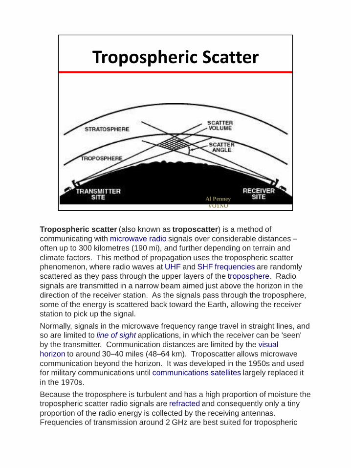
Tropospheric Scatter
Al Penney
VO1NO
Tropospheric scatter (also known as troposcatter) is a method of
communicating with microwave radio signals over considerable distances –often up to 300 kilometres (190 mi), and further depending on terrain and
climate factors. This method of propagation uses the tropospheric scatter phenomenon, where radio waves at UHF and SHF frequencies are randomly
scattered as they pass through the upper layers of the troposphere. Radio
signals are transmitted in a narrow beam aimed just above the horizon in the
direction of the receiver station. As the signals pass through the troposphere,
some of the energy is scattered back toward the Earth, allowing the receiver
station to pick up the signal.
Normally, signals in the microwave frequency range travel in straight lines, and so are limited to line of sight applications, in which the receiver can be 'seen'
by the transmitter. Communication distances are limited by the visual
horizon to around 30–40 miles (48–64 km). Troposcatter allows microwave
communication beyond the horizon. It was developed in the 1950s and used for military communications until communications satellites largely replaced it
in the 1970s.
Because the troposphere is turbulent and has a high proportion of moisture the tropospheric scatter radio signals are refracted and consequently only a tiny
proportion of the radio energy is collected by the receiving antennas. Frequencies of transmission around 2 GHz are best suited for tropospheric

scatter systems as at this frequency the wavelength of the signal interacts well with the moist, turbulent areas of the troposphere, improving signal to noise
ratios.
The basic mechanism of tropospheric scatter is shown in Figure 1. The
antennas of the two stations at the ends of the path cannot "see" each other,
but they can each "see" a common volume of the atmosphere, labeled in the
figure as the "scattering volume." Signals from one station are scattered by
atmospheric inhomogeneities in this region, and some of the scattering is in
the direction of the second station. The region of the atmosphere involved is
called the troposphere and it extends from the ground up to a height of about
15 km. It's the region in which all weather phenomena occurs, air- planes fly,
and is the region in which the "air" is found. Although this region looks clear
and uniform to the eye, it really contains a lot of turbulence and stratification.
Anyone who has had a bumpy ride in an aircraft has felt this first hand, just as
anyone who has seen a star twinkle has directly observed the optical effects of
atmospheric turbulence.
95

Propagation – 6M• 50 - 54 MHz
• Mix between HF and VHF propagation.
• Long range F2 propagation during solar peak.
• Sporadic E 1500 to 3000 km, Jun and Dec.
• Some Aurora.
• Moonbounce becoming popular.
Al Penney
VO1NO
The 6-meter band is the lowest portion of the very high frequency (VHF) radio
spectrum allocated to amateur radio use. The term refers to the average signal
wavelength of 6 meters.
Although located in the lower portion of the VHF band, it nonetheless occasionally displays propagation mechanisms characteristic of the high
frequency (HF) bands. This normally occurs close to sunspot maximum,
when solar activity increases ionization levels in the upper atmosphere. During
the last sunspot peak of 2005, worldwide 6-meter propagation occurred
making 6-meter communications as good as or in some instances and
locations, better than HF frequencies. The prevalence of HF characteristics on
this VHF band has inspired amateur operators to dub it the "magic band".
In the northern hemisphere, activity peaks from May through early August, when regular sporadic E propagation enables long-distance contacts spanning
up to 2,500 kilometres (1,600 mi) for single-hop propagation. Multiple-hop
sporadic E propagation allows intercontinental communications at distances of up to 10,000 kilometres (6,200 mi). In the southern hemisphere, sporadic E
propagation is most common from November through early February.
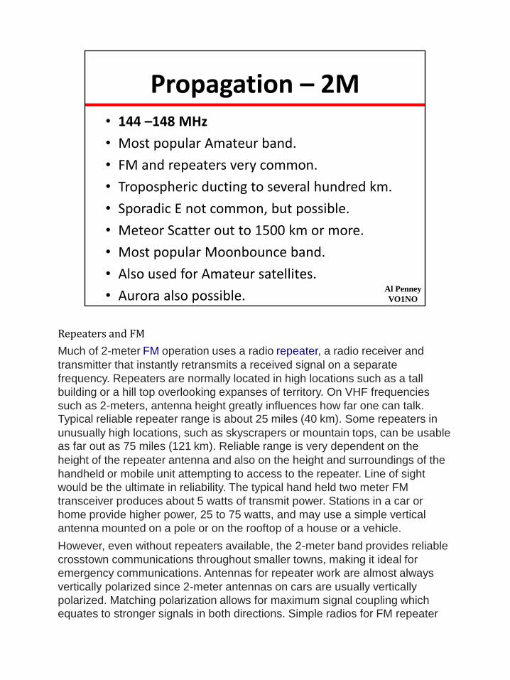
Propagation – 2M• 144 –148 MHz
• Most popular Amateur band.
• FM and repeaters very common.
• Tropospheric ducting to several hundred km.
• Sporadic E not common, but possible.
• Meteor Scatter out to 1500 km or more.
• Most popular Moonbounce band.
• Also used for Amateur satellites.
• Aurora also possible.Al Penney
VO1NO
Repeaters and FM
Much of 2-meter FM operation uses a radio repeater, a radio receiver and
transmitter that instantly retransmits a received signal on a separate
frequency. Repeaters are normally located in high locations such as a tall
building or a hill top overlooking expanses of territory. On VHF frequencies
such as 2-meters, antenna height greatly influences how far one can talk. Typical reliable repeater range is about 25 miles (40 km). Some repeaters in
unusually high locations, such as skyscrapers or mountain tops, can be usable as far out as 75 miles (121 km). Reliable range is very dependent on the
height of the repeater antenna and also on the height and surroundings of the
handheld or mobile unit attempting to access to the repeater. Line of sight
would be the ultimate in reliability. The typical hand held two meter FM
transceiver produces about 5 watts of transmit power. Stations in a car or
home provide higher power, 25 to 75 watts, and may use a simple vertical
antenna mounted on a pole or on the rooftop of a house or a vehicle.
However, even without repeaters available, the 2-meter band provides reliable
crosstown communications throughout smaller towns, making it ideal for
emergency communications. Antennas for repeater work are almost always
vertically polarized since 2-meter antennas on cars are usually vertically
polarized. Matching polarization allows for maximum signal coupling which equates to stronger signals in both directions. Simple radios for FM repeater

operation have become plentiful and inexpensive in recent years.
Communications beyond 50 miles
While the 2 meter band is best known as a local band using the FM mode,
there are many opportunities for long distance (DX) communications using
other modes. A well-placed antenna and high-power equipment can achieve
distances of up to a few hundred miles, and fortuitous propagation conditions
called "signal enhancements" can on occasion reach across oceans.
A set of two long Yagi antennas for the 2 meter band fed in phase to obtain
more gain and narrow main lobe of radiation (station WA6PY)
The typical 2 meter station using CW (Morse code) or SSB (single side band)
modes consists of a radio driving a power amplifier generating about 200–500 Watts of RF power. This extra power is usually fed to a multi-element,
compound antenna, usually a Yagi-Uda or Yagi, which can beam most of the
signal power towards the intended receiving station. "Beam antennas" provide substantial increase in signal directivity over ordinary dipole or vertical
antennas. Antennas used for distance work are usually horizontally polarized
instead of the vertical polarization customarily used for local contacts.
Stations that have antennas located in relatively high locations with views
(from the antenna) clear to the horizon have a big advantage over other stations. Such stations are able to communicate 100–300 miles (160–480 km)
consistently. It is usual for them to be heard at distances far beyond line of sight on a daily basis without help from signal enhancements. Signal
enhancements are unusual circumstances in the atmosphere and ionosphere
that bend the signal path into an arc that better follows the curve of the Earth,
instead of the radio waves traveling in the usual straight line off into space.
The best known of these are:
•tropospheric ducting
•sporadic E
•meteor scatter
These and other well-known forms of VHF signal enhancement that allow trans-oceanic and trans-continental contacts on 2 meters are described in the
subsections that follow within this section.
With the exception of sporadic E, directional antennas such as Yagis or log
periodic antennas are almost essential to take advantage of signal
enhancements. When a well-equipped station with its antenna well-located “high and in the clear” is operating during a signal enhancement, astonishing
distances can be bridged, momentarily approaching what is regularly possible
97

on shortwave and mediumwave.
Tropospheric ducting
Occasionally, signal bending in the atmosphere's troposphere known
as tropospheric ducting can allow 2 meter signals to carry hundreds or even
thousands of miles as evidenced by the occasional 2 meter contact between
the west coast of the United States and the Hawaiian Islands, the northeast
region to the Florida coast and across the Gulf of Mexico. These "Openings"
as they are known, are generally first spotted by amateurs operating SSB (Single Side Band) and CW (Continuous Wave) modes since amateurs using
these modes typically are attempting distance contacts (DX) and alert for
signal enhancement events.
Completion of contacts using these weak signal modes involves the exchange
of signal level reports and location by grid square which is known as the Maidenhead Locator System. Two way ducting contacts can have very
strong signals and are often made with moderate power, small antennas and
other types of modes. Long distance ducting contacts do occur using FM
modes as well but for the most part go unnoticed by many FM operators.
Sporadic E
Another form of VHF propagation is called Sporadic E propagation. This is a
phenomenon whereby radio signals are reflected back towards Earth by highly ionized segments of the ionosphere which can facilitate contacts in excess
of 1,000 miles (1,600 km) with very strong signals received by both parties.
Unlike some other long distance modes, high power and large antennas are often not required to make contact with distant stations via a sporadic E event.
A two-way conversation can take place over a distance of several hundred miles or more, often using low levels of RF power. Sporadic E is a rare and
completely random propagation phenomenon lasting anywhere from a matter
of minutes to several hours.
Satellite communications
Satellites are basically repeater stations in orbit. The 2 meter band is also used
in conjunction with the 70-centimeter band, or the 10-meter band and various
microwave bands via orbiting amateur radio satellites. This is known as cross
band repeating. On-board software defines what mode or band is in use at any
particular time and this is determined by amateurs at so-called earth stations
who control or instruct the satellite behavior. Amateurs know what mode is in
use via published internet schedules.
For instance, a favorite mode is Mode "B" or "V/U" which simply indicates the
uplink and downlink frequencies or bands the satellite is currently using. In this example, V/U means VHF/UHF or VHF uplink with UHF downlink. Most
97

amateur satellites are Low Earth Orbit satellites, or LEO's as they are
affectionately known, and generally are about 450 miles high (700 km). At that
height amateurs can expect reception distances of up to around 3,000 miles (4,800 km).
There are a few amateur satellites that have very high elliptical orbits. These satellites can reach altitudes of 30,000 miles (50,000 km) above the earth
where an entire hemisphere is visible providing outstanding communications
capabilities from any two points on the earth within line of sight of the satellite;
distances that are far beyond the reach of the LEO's.
Transequatorial propagation
Transequatorial propagation also known as (TEP) is a regular daytime occurrence on the 2 meter band over the equatorial regions and is common in
the temperate latitudes in late spring, early summer and, to a lesser degree, in early winter. For receiving stations located within ± 10 degrees of the
geomagnetic equator, equatorial E-skip can be expected on most days
throughout the year, peaking around midday local time.
Meteor burst
By speeding up Morse code using analog tape or digital modes such
as JT6M or FSK441, very short high-speed bursts of digital data can be
bounced off the ionized gas trail of meteor showers. The speed required to
confirm a two way contact via a short lived ionized meteor trail can only be
performed by fast computers on both ends with very little human interaction.
One computer will send a request for contact and if successfully received by a
distant station, a reply will be sent by the receiving stations computer usually
via the same ionized meteor trail to confirm the contact. If nothing is received
after the request, a new request is transmitted. This continues until a reply is
received to confirm the contact or until no contact can be made and no new
requests are sent. Using this high speed digital mode, a full two way contact,
can be completed in one second or less and can only be validated using a
computer. Depending on the intensity of the ionized meteor trail, multiple
contacts from multiple stations can be made off the same trail until it dissipates
and can no longer reflect VHF signals with sufficient strength. This mode is often called burst transmission and can yield communication distances similar
to sporadic E as described above.
Auroral propagation
Another phenomenon that produces upper atmosphere ionization suitable for 2-meter DXing are the auroras. Since the ionization persists much longer than
meteor trails, voice modulated radio signals may sometimes be used, but the constant movement of the ionized gas leads to heavy distortion of the signals
97
causing the audio to sound "ghostly" and whispered. In most instances using auroral reflections on 2 meters, audio or voice is totally unintelligible and ham
operators wishing to make contacts via aurora, must resort to CW (Morse
code).
CW signals returning from an auroral reflection have no distinct sound or tone
but simply sound like a swishing or whooshing noise. An exception to this phenomenon would be the 6 meter band which is significantly lower in
frequency than the 2 meter band by 94 MHz. In many instances 6 meter voice
modes are readable but with varying degrees of difficulty when reflected off an
aurora. Therefore, when using an auroral event as a radio signal reflector, the
reflected signal strength and signal intelligibility decreases with increasing
transmitting frequency.
Moonbounce (EME)
To communicate over the longest distances, hams use moon bounce. VHF
signals normally escape the Earth's atmosphere, so using the moon as a target
is quite practical. Due to the distance involved and the very high path loss
getting a readable signal bounced off the moon involves high power ~1,000 Watts and steerable high gain antennas. Receiving these very weak
return signals, again involves the use of high gain antennas (usually the same
ones used to transmit the signal) and a very low-noise front end RF amplifier
and a frequency stable receiver.
However, new and recent technological advances in weak signal detection has
allowed the successful reception of signals off the moon using much smaller or
less well equipped stations allowing reception of signals that are "in the noise" and not audible to the human ear. One of these modes is JT65 which is a
digital mode. Due to the delay of the signal traveling to the moon and back (travel time approx. 2.5 seconds), a person transmitting may hear the end of
their own transmission returning.
97

Propagation – 222 MHz• 222 – 225 MHz
• Somewhat neglected band.
• Becoming more popular however.
• Propagation generally similar to 2M.
• Sporadic E is rare however.
Al Penney
VO1NO

Propagation – 70cm• 430 – 450 MHz
• First Amateur band in UHF spectrum.
• Tropospheric ducting primary DX mode.
• FM, repeaters, Amateur Television.
• Sporadic E and Aurora rare.
• All Amateur bands from 70cm to 10 GHz are shared with other services.
Al Penney
VO1NO
70-centimeter propagation characteristics lie midway between 2-meter and 33-centimeter (~900 MHz) bands. Above 200 MHz, as frequency increases,
building penetration is reduced.[6] However, smaller obstacles may also block
or reflect the signal. Higher frequencies also present a lower noise floor,
making it easier to overcome both natural and artificial interference, especially
prevalent in urban environments.
Atmospheric thermal ducting is often more intense at UHF, because shorter
wavelengths have much greater refraction angles than longer ones. However,
a much stronger thermal inversion is often required than is needed for ducting
in the 2-meter band.

Questions?
Al Penney
VO1NO
100

What is the best method to tell if a band is “open” for communication with a particular distant location?
• Ask others on your local 2 metre FM repeater
• Telephone an experienced local amateur
• Look at the propagation forecasts in an amateur radio magazine
• Listen for signals from that area from an amateur beacon station or a foreign broadcast or television station on a nearby frequency
Review Question 1
Al Penney
VO1NO
101

What is the best method to tell if a band is “open” for communication with a particular distant location?
• Ask others on your local 2 metre FM repeater
• Telephone an experienced local amateur
• Look at the propagation forecasts in an amateur radio magazine
• Listen for signals from that area from an amateur beacon station or a foreign broadcast or television station on a nearby frequency
< Listen for signals from that area from an amateur beacon station or a foreign broadcast or television station on a nearby frequency >
Review Question 1
Al Penney
VO1NO
102
What type of propagation usually occurs from one hand-held VHF transceiver to another nearby?
• Auroral propagation
• Line-of-sight propagation
• Tunnel propagation
• Sky-wave propagation
Review Question 2
Al Penney
VO1NO
103

What type of propagation usually occurs from one hand-held VHF transceiver to another nearby?
• Auroral propagation
• Line-of-sight propagation
• Tunnel propagation
• Sky-wave propagation
< Line-of-sight propagation >
Review Question 2
Al Penney
VO1NO
104
How does the range of sky-wave propagation compare to ground-wave propagation?
• It is much longer
• It is much shorter
• It is about the same
• It depends on the weather
Review Question 3
Al Penney
VO1NO
105
How does the range of sky-wave propagation compare to ground-wave propagation?
• It is much longer
• It is much shorter
• It is about the same
• It depends on the weather
< It is much longer >
Review Question 3
Al Penney
VO1NO
106

When a signal is returned to Earth by the ionosphere, what is this called?
• Tropospheric propagation
• Ground-wave propagation
• Earth-Moon-Earth propagation
• Sky-wave propagation
Review Question 4
Al Penney
VO1NO
107
When a signal is returned to Earth by the ionosphere, what is this called?
• Tropospheric propagation
• Ground-wave propagation
• Earth-Moon-Earth propagation
• Sky-wave propagation
< Sky-wave propagation >
Review Question 4
Al Penney
VO1NO
108

How are VHF signals propagated within the range of the visible horizon?
• By direct wave
• By sky-wave
• By plane wave
• By geometric wave
Review Question 5
Al Penney
VO1NO
109
How are VHF signals propagated within the range of the visible horizon?
• By direct wave
• By sky-wave
• By plane wave
• By geometric wave
< By direct wave >
Review Question 5
Al Penney
VO1NO
110

Sky-wave is another name for:
• inverted wave
• ionospheric wave
• tropospheric wave
• ground wave
Review Question 6
Al Penney
VO1NO
111

Sky-wave is another name for:
• inverted wave
• ionospheric wave
• tropospheric wave
• ground wave
< ionospheric wave >
Review Question 6
Al Penney
VO1NO
112

Review Question 7
Al Penney
VO1NO
What two sub-regions of ionosphere exist only in the daytime?
• Electrostatic and electromagnetic
• D and E
• F1 and F2
• Troposphere and stratosphere
113
Review Question 7
Al Penney
VO1NO
What two sub-regions of ionosphere exist only in the daytime?
• Electrostatic and electromagnetic
• D and E
• F1 and F2
• Troposphere and stratosphere
< F1 and F2>
114

At lower HF frequencies, radiocommunication out to 200 km is made possible by:
• troposphere
• skip wave
• ionosphere
• ground wave
Review Question 8
Al Penney
VO1NO
115

At lower HF frequencies, radiocommunication out to 200 km is made possible by:
• troposphere
• skip wave
• ionosphere
• ground wave
< ground wave >
Review Question 8
Al Penney
VO1NO
116

The distance travelled by ground waves:
• is more at higher frequencies
• is the same for all frequencies
• is less at higher frequencies
• depends on the maximum usable frequency
Review Question 9
Al Penney
VO1NO
117

The distance travelled by ground waves:
• is more at higher frequencies
• is the same for all frequencies
• is less at higher frequencies
• depends on the maximum usable frequency
< is less at higher frequencies >
Review Question 9
Al Penney
VO1NO
118

What causes the ionosphere to form?
• Lightning ionizing the outer atmosphere
• Release of fluorocarbons into the atmosphere
• Temperature changes ionizing the outer atmosphere
• Solar radiation ionizing the outer atmosphere
Review Question 10
Al Penney
VO1NO
119

What causes the ionosphere to form?
• Lightning ionizing the outer atmosphere
• Release of fluorocarbons into the atmosphere
• Temperature changes ionizing the outer atmosphere
• Solar radiation ionizing the outer atmosphere
< Solar radiation ionizing the outer atmosphere >
Review Question 10
Al Penney
VO1NO
120
Reception of high frequency (HF) radio waves beyond 4000 km is generally made possible by:
• ground wave
• skip wave
• surface wave
• ionospheric wave
Review Question 11
Al Penney
VO1NO
121

Reception of high frequency (HF) radio waves beyond 4000 km is generally made possible by:
• ground wave
• skip wave
• surface wave
• ionospheric wave
< ionospheric wave >
Review Question 11
Al Penney
VO1NO
122

When is the ionosphere least ionized?
• Shortly before midnight
• Shortly before dawn
• Just after noon
• Just after dusk
Review Question 12
Al Penney
VO1NO
123

When is the ionosphere least ionized?
• Shortly before midnight
• Shortly before dawn
• Just after noon
• Just after dusk
< Shortly before dawn >
Review Question 12
Al Penney
VO1NO
124

Why is the F2 region mainly responsible for the longest distance radio-wave propagation?
• Because it is the lowest ionospheric region
• Because it does not absorb radio waves as much as other ionospheric regions
• Because it is the highest ionospheric region
• Because it exists only at night
Review Question 13
Al Penney
VO1NO
125

Why is the F2 region mainly responsible for the longest distance radio-wave propagation?
• Because it is the lowest ionospheric region
• Because it does not absorb radio waves as much as other ionospheric regions
• Because it is the highest ionospheric region
• Because it exists only at night
< Because it is the highest ionospheric region >
Review Question 13
Al Penney
VO1NO
126

What is the main reason the 160, 80 and 40 metre amateur bands tend to be useful only for
short-distance communications during daylight hours?
• Because of magnetic flux
• Because of a lack of activity
• Because of D-region absorption
• Because of auroral propagation
Review Question 14
Al Penney
VO1NO
127

What is the main reason the 160, 80 and 40 metre amateur bands tend to be useful only for
short-distance communications during daylight hours?
• Because of magnetic flux
• Because of a lack of activity
• Because of D-region absorption
• Because of auroral propagation
< Because of D-region absorption >
Review Question 14
Al Penney
VO1NO
128

What is a skip zone?
• An area which is too far away for ground-wave propagation, but too close for sky-wave propagation
• An area which is too far away for ground-wave or sky-wave propagation
• An area covered by sky-wave propagation
• An area covered by ground-wave propagation
Review Question 15
Al Penney
VO1NO
129
What is a skip zone?
• An area which is too far away for ground-wave propagation, but too close for sky-wave propagation
• An area which is too far away for ground-wave or sky-wave propagation
• An area covered by sky-wave propagation
• An area covered by ground-wave propagation
< An area which is too far away for ground-wave propagation, but too close for sky-wave propagation>
Review Question 15
Al Penney
VO1NO
130

What is the maximum distance along the Earth’s surface that is normally covered in one hop using the F2 region?
• 4000 km (2500 miles)
• None; the F2 region does not support radio-wave propagation
• 2000 km (1250 miles)
• 300 km (190 miles)
Review Question 16
Al Penney
VO1NO
131

What is the maximum distance along the Earth’s surface that is normally covered in one hop using the F2 region?
• 4000 km (2500 miles)
• None; the F2 region does not support radio-wave propagation
• 2000 km (1250 miles)
• 300 km (190 miles)
< 4000 km (2500 miles) >
Actually this value can be as high as 4800 km! But remember the answer IC wants.
Review Question 16
Al Penney
VO1NO
132

What is the maximum distance along the Earth’s surface that is normally covered in one hop using the E region?
• 2000 km (1250 miles)
• 300 km (190 miles)
• 4000 km (2500 miles)
• None; the E region does not support radio-wave propagation
Review Question 17
Al Penney
VO1NO
133

What is the maximum distance along the Earth’s surface that is normally covered in one hop using the E region?
• 2000 km (1250 miles)
• 300 km (190 miles)
• 4000 km (2500 miles)
• None; the E region does not support radio-wave propagation
< 2000 km (1250 miles) >
Review Question 17
Al Penney
VO1NO
134

The distance to Europe from your location is approximately 5000 km. What sort of propagation is the most likely to be involved?
• Back scatter
• Tropospheric scatter
• Multihop
• Sporadic “E”
Review Question 18
Al Penney
VO1NO
135

The distance to Europe from your location is approximately 5000 km. What sort of propagation is the most likely to be involved?
• Back scatter
• Tropospheric scatter
• Multihop
• Sporadic “E”
< Multihop >
Review Question 18
Al Penney
VO1NO
136
The distance from the transmitter to the nearest point where the sky wave returns to the Earth is called the:
• maximum usable frequency
• skip distance
• skip zone
• angle of radiation
Review Question 19
Al Penney
VO1NO
137

The distance from the transmitter to the nearest point where the sky wave returns to the Earth is called the:
• maximum usable frequency
• skip distance
• skip zone
• angle of radiation
< skip distance >
Review Question 19
Al Penney
VO1NO
138

The skip distance of a sky wave will be greatest when the:
• polarization is vertical
• ionosphere is most densely ionized
• signal given out is strongest
• angle between ground and radiation is smallest
Review Question 20
Al Penney
VO1NO
139

The skip distance of a sky wave will be greatest when the:
• polarization is vertical
• ionosphere is most densely ionized
• signal given out is strongest
• angle between ground and radiation is smallest
< angle between ground and radiation is smallest >
Review Question 20
Al Penney
VO1NO
140

What effect does the D region of the ionosphere have on lower frequency HF signals in the daytime?
• It refracts the radio waves back to Earth
• It has little or no effect on 80-metre radio waves
• It absorbs the signals
• It bends the radio waves out into space
Review Question 21
Al Penney
VO1NO
141

What effect does the D region of the ionosphere have on lower frequency HF signals in the daytime?
• It refracts the radio waves back to Earth
• It has little or no effect on 80-metre radio waves
• It absorbs the signals
• It bends the radio waves out into space
< It absorbs the signals >
Review Question 21
Al Penney
VO1NO
142

Two or more parts of the radio wave follow different paths during propagation and this may result in phase differences at the receiver. This “change” at the receiver is called:
• absorption
• skip
• fading
• baffling
Review Question 22
Al Penney
VO1NO
143

Two or more parts of the radio wave follow different paths during propagation and this may result in phase differences at the receiver. This “change” at the receiver is called:
• absorption
• skip
• fading
• baffling
< fading >
Review Question 22
Al Penney
VO1NO
144

The usual effect of ionospheric storms is to:
• increase the maximum usable frequency
• cause a fade-out of sky-wave signals
• produce extreme weather changes
• prevent communications by ground wave
Review Question 23
Al Penney
VO1NO
145

The usual effect of ionospheric storms is to:
• increase the maximum usable frequency
• cause a fade-out of sky-wave signals
• produce extreme weather changes
• prevent communications by ground wave
< cause a fade-out of sky-wave signals >
Review Question 23
Al Penney
VO1NO
146

On the VHF and UHF bands, polarization of the receiving antenna is very important in relation to the transmitting antenna, yet on HF bands it is relatively unimportant. Why is that so?
• Greater selectivity is possible with HF receivers making changes in polarization redundant
• The ionosphere can change the polarization of the signal from moment to moment
• The ground wave and the sky wave continually shift the polarization
• Anomalies in the Earth’s magnetic field produce a profound effect on HF polarization but not on VHF & UHF frequencies
Review Question 24
Al Penney
VO1NO
147

On the VHF and UHF bands, polarization of the receiving antenna is very important in relation to the transmitting antenna, yet on HF bands it is relatively unimportant. Why is that so?
• Greater selectivity is possible with HF receivers making changes in polarization redundant
• The ionosphere can change the polarization of the signal from moment to moment
• The ground wave and the sky wave continually shift the polarization
• Anomalies in the Earth’s magnetic field produce a profound effect on HF polarization but not on VHF & UHF frequencies
< The ionosphere can change the polarization of the signal from moment to moment >
Review Question 24
Al Penney
VO1NO
148

How does the bandwidth of a transmitted signal affect selective fading?
• It is the same for both wide and narrow bandwidths
• Only the receiver bandwidth determines the selective fading effect
• It is more pronounced at narrow bandwidths
• It is more pronounced at wide bandwidths
Review Question 25
Al Penney
VO1NO
149

How does the bandwidth of a transmitted signal affect selective fading?
• It is the same for both wide and narrow bandwidths
• Only the receiver bandwidth determines the selective fading effect
• It is more pronounced at narrow bandwidths
• It is more pronounced at wide bandwidths
< It is more pronounced at wide bandwidths >
Review Question 25
Al Penney
VO1NO
150

How do sunspots change the ionization of the atmosphere?
• The more sunspots there are, the greater the ionization
• The more sunspots there are, the less the ionization
• Unless there are sunspots, the ionization is zero
• They have no effect
Review Question 26
Al Penney
VO1NO
151

How do sunspots change the ionization of the atmosphere?
• The more sunspots there are, the greater the ionization
• The more sunspots there are, the less the ionization
• Unless there are sunspots, the ionization is zero
• They have no effect
< The more sunspots there are, the greater the ionization >
Review Question 26
Al Penney
VO1NO
152

What influences all radio communication beyond ground-wave or line-of-sight ranges?
• The F2 region of the ionosphere
• The F1 region of the ionosphere
• Lunar tidal effects
• Solar radiation
Review Question 27
Al Penney
VO1NO
153

What influences all radio communication beyond ground-wave or line-of-sight ranges?
• The F2 region of the ionosphere
• The F1 region of the ionosphere
• Lunar tidal effects
• Solar radiation
< Solar radiation >
Review Question 27
Al Penney
VO1NO
154

The ability of the ionosphere to reflect high frequency radio signals depends on:
• the receiver sensitivity
• upper atmosphere weather conditions
• the amount of solar radiation
• the power of the transmitted signal
Review Question 28
Al Penney
VO1NO
155

The ability of the ionosphere to reflect high frequency radio signals depends on:
• the receiver sensitivity
• upper atmosphere weather conditions
• the amount of solar radiation
• the power of the transmitted signal
< the amount of solar radiation >
Review Question 28
Al Penney
VO1NO
156
What does maximum usable frequency mean?
• The lowest frequency signal that will reach its intended destination
• The highest frequency signal that is most absorbed by the ionosphere
• The lowest frequency signal that is most absorbed by the ionosphere
• The highest frequency signal that will reach its intended destination
Review Question 29
Al Penney
VO1NO
157

What does maximum usable frequency mean?
• The lowest frequency signal that will reach its intended destination
• The highest frequency signal that is most absorbed by the ionosphere
• The lowest frequency signal that is most absorbed by the ionosphere
• The highest frequency signal that will reach its intended destination
< The highest frequency signal that will reach its intended destination >
Review Question 29
Al Penney
VO1NO
158

At what point in the solar cycle does the 20-metre band usually support worldwide propagation during daylight hours?
• Only at the maximum point of the solar cycle
• At the summer solstice
• At any point in the solar cycle
• Only at the minimum point of the solar cycle
Review Question 30
Al Penney
VO1NO
159

At what point in the solar cycle does the 20-metre band usually support worldwide propagation during daylight hours?
• Only at the maximum point of the solar cycle
• At the summer solstice
• At any point in the solar cycle
• Only at the minimum point of the solar cycle
< At any point in the solar cycle >
Review Question 30
Al Penney
VO1NO
160

During summer daytime, which bands are the most difficult for communications beyond ground wave?
• 20 metres
• 160 and 80 metres
• 40 metres
• 30 metres
Review Question 31
Al Penney
VO1NO
161
During summer daytime, which bands are the most difficult for communications beyond ground wave?
• 20 metres
• 160 and 80 metres
• 40 metres
• 30 metres
<160 and 80 metres >
Review Question 31
Al Penney
VO1NO
162

What causes tropospheric ducting of radio waves?
• A temperature inversion
• Lightning between the transmitting and receiving stations
• An aurora to the north
• A very low pressure area
Review Question 32
Al Penney
VO1NO
163

What causes tropospheric ducting of radio waves?
• A temperature inversion
• Lightning between the transmitting and receiving stations
• An aurora to the north
• A very low pressure area
< A temperature inversion >
Review Question 32
Al Penney
VO1NO
164

Where in the ionosphere does auroral activity occur?
• At D-region height
• At E-region height
• At F-region height
• In the equatorial band
Review Question 33
Al Penney
VO1NO
165

Where in the ionosphere does auroral activity occur?
• At D-region height
• At E-region height
• At F-region height
• In the equatorial band
< At E-region height >
Review Question 33
Al Penney
VO1NO
166

Excluding enhanced propagation modes, what is the approximate range of normal VHF tropospheric propagation?
• 1600 km (1000 miles)
• 800 km (500 miles)
• 2400 km (1500 miles)
• 3200 km (2000 miles)
Review Question 34
Al Penney
VO1NO
167

Excluding enhanced propagation modes, what is the approximate range of normal VHF tropospheric propagation?
• 1600 km (1000 miles)
• 800 km (500 miles)
• 2400 km (1500 miles)
• 3200 km (2000 miles)
< 800 km (500 miles) >
Review Question 34
Al Penney
VO1NO
168

What kind of unusual HF propagation allows weak signals from the skip zone to be heard occasionally?
• Sky-wave with low radiation angle
• Ducting
• Ground-wave
• Scatter-mode
Review Question 35
Al Penney
VO1NO
169

What kind of unusual HF propagation allows weak signals from the skip zone to be heard occasionally?
• Sky-wave with low radiation angle
• Ducting
• Ground-wave
• Scatter-mode
< Scatter-mode >
Review Question 35
Al Penney
VO1NO
170

Which of the following IS NOT a scatter mode?
• Tropospheric scatter
• Ionospheric scatter
• Absorption scatter
• Meteor scatter
Review Question 36
Al Penney
VO1NO
171
Which of the following IS NOT a scatter mode?
• Tropospheric scatter
• Ionospheric scatter
• Absorption scatter
• Meteor scatter
< Absorption scatter >
Review Question 36
Al Penney
VO1NO
172

For Next Class:
• Review Chapter 6 of Basic Study Guide;
• Read Chapter 7 of Basic Study Guide;
• Read the Question Bank – there are lots more questions on propagation; and
• Read RIC-9: https://www.ic.gc.ca/eic/site/smt-gst.nsf/eng/sf02102.html
173

174
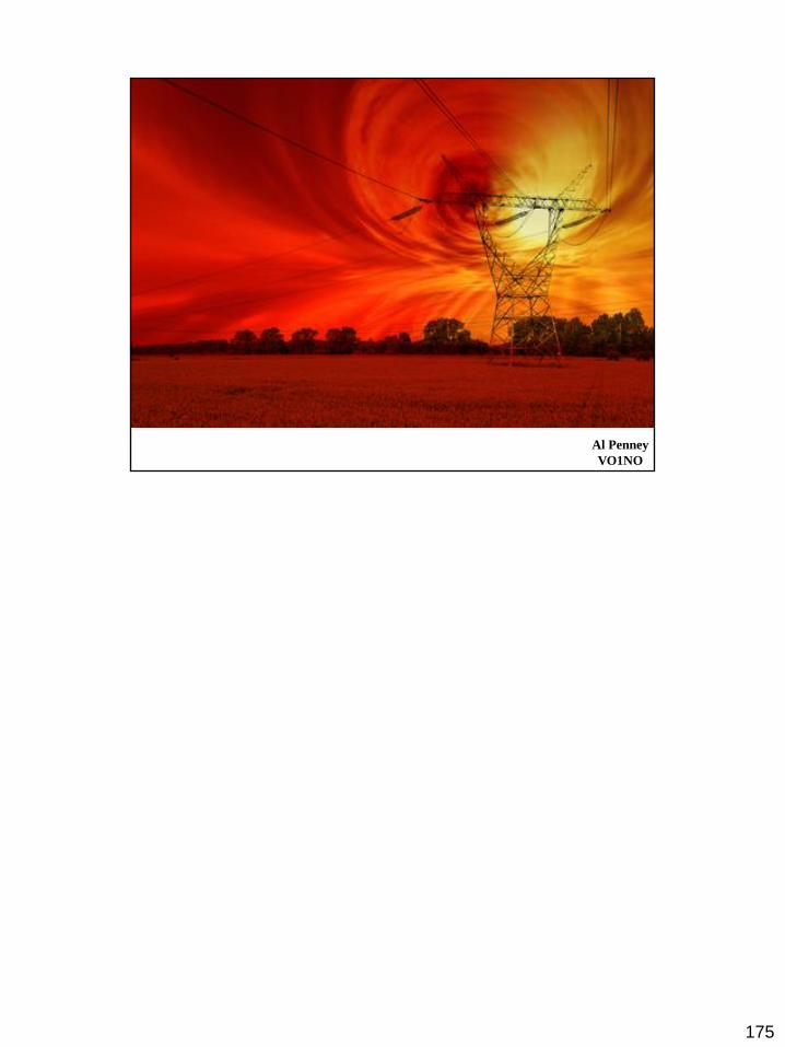
Al Penney
VO1NO
175

Al Penney
VO1NO
176

Al Penney
VO1NO
177

178

Al Penney
VO1NO
179

Al Penney
VO1NO
180

Al Penney
VO1NO
181

Al Penney
VO1NO
182

Al Penney
VO1NO
183

Al Penney
VO1NO
184

Al Penney
VO1NO
185

Al Penney
VO1NO
186
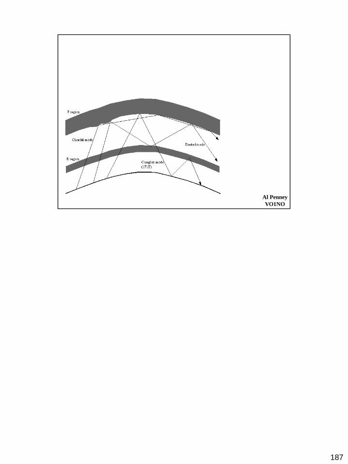
Al Penney
VO1NO
187

Al Penney
VO1NO
188