Chapter 6 Nonlinear Systems Random Processes

《Random Signal Processing》 Chapter6 Nonlinear Systems Random Processes

Chapter 6 Nonlinear Systems Random Processes

Contents

6. Nonlinear Systems: Random Processes ...........................................................................................2 6.1 Introduction.......................................................................................................................................... 2

6.2 Classification of Nonlinear Systems.................................................................................................... 2

6.2.1 Zero-memory Nonlinear Systems ............................................................................................................. 2

6.2.2 Bilinear Systems ....................................................................................................................................... 3

6.2.3 Trilinear Systems....................................................................................................................................... 8

6.2.4 Volterra Representation for General Nonlinear Systems........................................................................... 9

6.3 Random Outputs for Instantaneous Nonlinear System ...................................................................... 10

6.3.1 First-Order Density for Instantaneous Nonlinear Systems...................................................................... 11

6.3.2 Mean of the Output Process .................................................................................................................... 12

6.3.3 Second-Order Densities for Instantaneous Nonlinearities ...................................................................... 13

6.3.4 Autocorrelation Function for Instantaneous Nonlinear Systems............................................................. 14

6.3.5 Higher-Order Moments ........................................................................................................................ 17

6.3.6 Stationarity of Output Process.............................................................................................................. 17

6.4 Characterizations for Bilinear Systems.............................................................................................. 17

6.4.1 Mean of the Output of a Bilinear System................................................................................................ 18

6.4.2 Cross-correlation between Input and Output of a Bilinear System ......................................................... 18

6.4.3 Autocorrelation Function for the Output of a Bilinear System ............................................................... 18

6.5 Characterizations for Trilinear Systems............................................................................................. 19

6.5.1 Mean of the Output of a Trilinear System............................................................................................... 19

6.5.2 Cross-correlation between Input and Output of a Trilinear System ........................................................ 19

6.5.3 Autocorrelation Function for the Output of a Trilinear System............................................................... 19

6.6Characterizations for Volterra Nonlinear Systems.............................................................................. 20

6.7 Higher-order Characterizations.......................................................................................................... 21

6.7.1 Moment Function for Random Processes ............................................................................................... 21

6.7.2 Cumulant Function for Random Processes ............................................................................................. 22

6.7.3 Polyspectrum for Random Processes ...................................................................................................... 23

6.8 Summary............................................................................................................................................ 24

Xidian University Liu Congfeng E-Mail:[email protected] Page 1 of 24


6. Nonlinear Systems: Random Processes

6.1 Introduction

In Chapter 5 the input-output characteristics were explored for a linear system excited by a random process. It was

seen that the mean of the input process was sufficient to determine the mean of the output process, and

correspondingly the autocorrelation function of the input was sufficient to determine the autocorrelation function

of the output process. However, there are many elements and systems, especially in communication theory, that

are not linear, for example, devices like hard and soft limiters, rectifiers, modulators, and demodulators.

For these type of nonlinearities the autocorrelation functions are, in general, no longer sufficient to

characterize the output autocorrelation functions, so it its necessary to introduce the concepts of higher-order

correlation functions, cumulants, and higher-order spectrums. This chapter will also identify various classes of

nonlinear systems and analyze them with respect to establishing input-output statistical relationships. The

presentation will be guided more by what is mathematically tractable than what would be a complete and

thorough investigation.

6.2 Classification of Nonlinear Systems

Currently no general theory exists that can handle all types of nonlinear systems. Therefore our presentation will

contain special methods for analyzing certain classes of nonlinear systems. A hierarchical classification of

nonlinear systems has been presented in Zadeh, and although we do not specifically use his nomenclature (type 0,

type 1 etc.), the classes we present follow his lower-order classification. Our discussion will include instantaneous

nonlinearities(type 0), and various cascades of linear systems and instantaneous nonlinear systems(type 1),

including bilinear and trilinear cases. The chapter will conclude with a brief introduction to Volterra functionals

for representing general nonlinear systems. The discussion begins with memoryless or zero-memory nonlinear

systems.

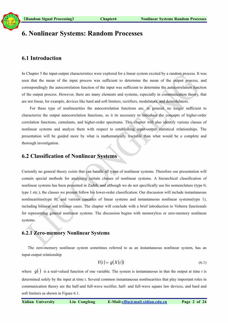
6.2.1 Zero-memory Nonlinear Systems

The zero-memory nonlinear system sometimes referred to as an instantaneous nonlinear system, has an

input-output relationship

tXgtY (6.1)

where is a real-valued function of one variable. The system is instantaneous in that the output at time t is

determined solely by the input at time t. Several common instantaneous nonlinearities that play important roles in

communication theory are the half-and full-wave rectifier, half- and full-wave square law devices, and hard and

soft limiters as shown in Figure 6.1.

g



x x

y=g(x) y=g(x) )

(a) (b)

Figure 6.1 Common instantaneous nonlinearities

x

y=g(x)

(c)

x

(d)

x x

y=g(x) y=g(x) )

(e) (f)

x

y=g(x)

(g) (h)

x

y=g(x))

y=g(x))

(a) quantizer, (b) half wave rectifier, (c) square law half wave device, (d)hard limiter, (e)saturation, (f)full wave rectifier, (g)square law full wave device, (h)soft limiter.

6.2.2 Bilinear Systems

A bilinear system as described by Bendat is a special case of a general Volterra system(to be discussed later),

and its input and output are governed by the following integral equation:

(6.2) 21212122 )()(),( ddtxtxhtxLty

The system is specified, with respect to input and output, by ),( 212 h , which is called the time domain kernel.

Notice that if 1 and 2 are interchanged in the integral, the output can be rearranged as follows:

2121212 )()(),()( ddtxtxhty

(6.3)

Since the is still the same, it is seen that the time domain darnel must be symmetrical to have a unique

output, that is,

)(ty

),(),( 212212 hh (6.4)

If the input is a sum of two inputs, txtx 21 , the output from Eq. (6.2) is )(ty

2122211211212 )]()()][()([),()( ddtxtxtxtxhty

(6.5)

By expanding out the product and using the symmetric property of ),( 212 h , we obtain an output that is the


《Random Signal Processing》 Chapter6 Nonlinear Systems Random Processes sum of responses of the system to and tx1 tx2

2

)](tax

0

each separately and another term involving the integration

of the time domain kernel and the cross product of the two signals as

212211212212 )]()(),()]()]([)( ddtxtxhttxLty

2[xL

,( 12

(6.6)

Therefore, unless the integral term is zero for all time, superposition does not hold for a bilinear system,

exemplifying the fact that the system is not a linear system.

Similarly it is easy to show that the response of the system to an input equal to a·x (t), where is a constant

is

a

(6.7) )]([[ 22

2 txLaL

The two properties are given in Eqs.(6.6) and (6.7) are sometimes used as an alternative definition for a bilinear

system.

A bilinear system is causal if )2 h for all 1 and 02 . In taking the absolute values of both

sides of (6.2), it is possible to see that the bilinear system will give a bounded output if the input is bounded. Thus

the bilinear system will be BIBO stable provided that

Bddh

()2 t

212 21 ),(

(t

where B is finite (6.8)

If the input to the bilinear system specified in Eq. (6.2) is a delta function, the output will be

),()(),()),()( 22222212112 tthdtthddhty

(6.9)

Thus the response to a delta function is not the time domain kernel but is the time domain kernel evaluated on the

line t 21 . Knowing the kernel on just that line is not sufficient information for characterizing the system

with respect to input and output, and thus a bilinear system cannot be identified by knowing only its impulse

response as was true for a linear system.


The frequency domain kernel )2,1(2 jH

1, jj

j for a bilinear system is defined as the two-dimensional Fourier

transform of the time domain kernel as follows:

21)(

212222211),()( ddehH j

(6.10)

Characterizing a bilinear system means that we specify either the time domain or frequency domain kernels.

Several examples of bilinear systems will be presented. They include a square law device, a square law device, a

square law device followed by a linear system, a linear system followed by a square law device and the cascade of

linear system, a square law device and linear system. Each of these systems will be examined and the time domain

kernels developed for their characterizations by using (6.10).

If the ) -( 1tx and ) -( 2tx are replaced in (6.10) by their inverse Fourier transforms, the output

is seen to be

)(ty

2121212212

212)(

21)(

11)212

22112211

221

),()(4

1

)(2

1(

2

1),()(

()

deeddeehjX

dddejXdjhty

jjjj

tjt

jX

X

e j

(6.11)

《Random Signal Processing》 Chapter6 Nonlinear Systems Random Processes The term in square brackets is the frequency domain kernel 212 , jjH , the first double integral gives the

two-dimensional inverse Fourier transform of the product 1jX , and 2jX but evaluated at times t1 and

t2 , both equaling t. Thus can be finally written as )(ty

tttt

jjHjXjXFty

21 ,21221

1 ),()()()( (6.12)

In this way it is seen not to be a product of the two-dimensional transforms, so the frequency domain kernel

cannot be thought of as the frequency response of the bilinear system.

If we take the one-dimensional Fourier transform directly of the output given in the basic definition (6.2), we

obtain

2121212

2121212

)()(),(

)()(),()]([

dddtettxh

dteddtxtxhtyF

tj

tj

(6.13)

The term in parentheses is the one-dimensional Fourier transform of the product of the two time-translated

versions of the input signal and thus is a function of both )(tx 1 and 2 . Since this term in parentheses cannot

be taken outside the integral signs, it is seen that the result is not the product of the transforms.

Square Law System. Let and represent the input and output, respectively, of a square law system

as shown in Figure 6.2 and governed by the following input-output relationship:

)(tx )(ty

(6.14) )()( 2 txty

A logical question at this time is: Is this system a bilinear system and if so what time domain kernel characterizes

it? To answer this question, is written in terms of a delta function as )(tx

(6.15) 111 )()()( dtxtx

Substituting this expression for into (6.14) and rearranging allows the output to be written as )(tx

(6.16)

212121

2221112

))(()()(

)()()()()()(

ddttx

dtxdtxtxty

It is seen that the nonlinear square law system is in the proper integral form,(6.2), and the product of the delta

functions can be identified as the time domain kernel

)()(),( 21212 h (6.17)

(·)2x(t) y(t)

Figure 6.2 A square law device

The two-dimensional frequency domain dernel can be obtained by taking the Fourier transform of the time

domain kernel, which for the ),( 212 h above gives


《Random Signal Processing》 Chapter6 Nonlinear Systems Random Processes 1),( 21 jjH for all 1 and 2 (6.18)

Care should be used in interpreting this result as the frequency response of the system for it doesn’t represent

the same information as the frequency response for the linear system. It is wrong to assume that it means that all

signals are passed without alteration , as is the case for an all pass linear system. This is hardly the case for, if the

Fourier transform of is taken, it becomes )(ty

)(*)()]([)]([ 22 jXjXtxFtyF (6.19)

Thus the output transform is seen as the convolution of the Fourier transform of the input with itself. This will

certainly give a different output transform, and as convolution has a tendency to broaden, the square law device

actually creates new output frequency content outside the frequency range of the input. This result is typical of

nonlinear systems in general.

Linear System Followed by a Square Law Device. Many nonlinear systems can be modeled as a nomemory

nonlinear filter followed by a linear system, and the resulting system is no longer memoryless. A special case of

this type of system is where the nonlinearity is a square law device as shown in Figure 6.3.

h(t)

y(t) (·)2x(t)

Figure 6.3 Linear system followed by a Square law device

The output for this case can be written in terms of the impulse response of the linear system as )(ty

2121212 )()()()(])()([)( ddtxtxhhdtxhty

(6.20)

Thus the linear system followed by a square law device is a bilinear system and the time domain kernel is

recognized from Eq.(6.2) as

)()(),( 2121 hhh (6.21)

The corresponding frequency domain kernel obtained by taking the two-dimensional transform of the time

domain kernel given in Eq.(6.21), is easily seen to be the product of the frequency responses of the linear portions

of the bilinear system in each of the variables as

)()(),( 21212 jHjHjjH (6.22)

This doesn’t mean that the frequency response of this particular bilinear system is a product of the frequency

response of the bilinear system; it simply gives the frequency domain kernel.

Square Law Device Followed by a Linear System. Another combination that comes up frequently is a nonlinear

system that is a no memory device followed by a linear system. The special case where the instantaneous system

is a square law device is shown in Figure 6.4.




To obtain the time domain kernel for this type of nonlinear system the output of the system above is first

written as

112

1)()( dtxhty

(6.23)

This can be put in the form of a bilinear system by rewriting tx2 in terms of a delta function as

2122112 )()()()( dtxtxtx

(6.24)

Substituting (6.24) into (6.23) and rearranging gives

2121121 )()()()()( ddtxtxhty

(6.25)

Thus the system specified above is a bilinear system and can be characterized by its time domain kernel as

)()(),( 121212 hh (6.26)

The time domain kernel is seen to be nonzero only on the line 12 , and thus is symmetric by force. By

taking the two-dimensional transform of the time domain kernel, the corresponding frequency domain kernel is

given by

)()(

)()(),(

211)(

1

21)(

121212

2211

2211

jHdeh

ddehjjH

j

j

(6.27)

Thus the frequency domain kernel for this type of nonlinear system is obtained by taking the Fourier transform of

the linear system represented by jH and replacing the by the sum 21 .

Cascade Linear System-Square Law Device-Linear System. The cascade of a linear system, square law device,

and linear system is shown in Figure 6.5. If and represent the impulse responses of the pre- and

postfilter, respectively, it is possible to show with a development similar to the two preceding sections that

)(1 th )(2 th

dhhhh

)()()(),( 22111212 (6.28)

Thus this cascade is a bilinear system as well.

h2 (t)

y(t)

Figure 6.5 Bilinear system composed of a cascade of linear system-squarer-linear system

x(t) (·)2h1(t)

h(t)

y(t)

Figure 6.4 Square law device followed by a Linear time invariant system

(·)2x(t)

《Random Signal Processing》 Chapter6 Nonlinear Systems Random Processes By taking the two-dimensional Fourier transform of (6.28), we can see that the frequency domain kernel of

this cascade system is given by

)()()(),( 2122111212 jHjHjHjjH (6.29)

6.2.3 Trilinear Systems

The input-output relationship for a trilinear system, described clearly in Bendat[1], is defined as


3213213213 )()()(),,()]([)( dddtxtxtxhtxLty

(6.30)

Where ),,( 3213 h is the third-order time domain kernel, and its specification characterizes the system with

respect to input-output relationship.

It can be shown, with developments similar to those of the previous sections, that a cuber, and a cuber

followed by a linear time-invariant system, and a linear time-invariant system followed by a cuber, and a cascade

of linear system, cuber, and linear system, are all special cases of trilinear systems. These special cases are shown

in Figure 6.6, and the resulting time domain kernels for these special cases are summarized below:

dhhhhhlinearcuberLinear

hhhhcuberLinear

hhlinearCube

hCuber

)()()()(),,(:

)()()(),,(:

)()()(),,(:

)()()(),,(:

23121113213

3322113213

3121123213

3213213

(6.31)

y(t) (·)3x(t) h1(t)

(b) Cuber-linear system

h2 (t)

(·)3

(a) Cuber

x(t) (·)3y(t)

x(t) y(t)

(d) Cascade: linear system-squarer-linear system

(c) Linear system-cuber

h2 (t)

y(t) (·)3h1(t)

x(t)

Figure 6.6 Special Trilinear systems

Their corresponding frequency domain kernels, obtained by taking the three-dimensional Fourier transform of

the time domain kernels can be determined as follows:


)()()()(),,(:

)()()(),,(:

)(),,(:

1),,(:

32123121113213

3121113213

32123213

3213

jHjHjHjHjjjHlinearcuberLinear

jHjHjHjjjHcuberLinear

jHjjjHlinearCube

jjjHCuber

(6.32)

6.2.4 Volterra Representation for General Nonlinear Systems

Volterra showed that the relationship between input tx and output ty for any nonlinear, causal,

time-invariant, finite memory, analytic system, can be written as

...)()()(),,,(

...)()(),()()()(

21210 0 0 21

21210 0 21210 1110

nnnn dddtxtxtxk

ddtxtxkdtxkkty

(6.33)

The output is an infinite sum of a constant and other terms containing one, two, and k-dimensional

integrals. The output is thus written as

ty

)()()()( 210 tytytyyty n (6.34)

and can be viewed as the sum of the responses from each kernel as shown in Figure 6.7. The first term is a

constant and can usually be subtracted off without loss of generality, the second term is a convolution integral

representing the linear portion, and the other terms are deviations from the linear at various levels. The , 0k

)( 11 k ,…, ),,,( 21 nnk are called the first, second, and nth-order time domain kernels of the system.

From Eq.(6.33) it can be seen that knowing the kernels is sufficient information for the determination of the

output for any given input.

y0

y1(t)

0k


The part of the output appears as a convolution of the input with the first-order Volterra kernel and )(1 ty

y2(t)

yn(t)

y(t)

x(t)

Figure 6.7 The Volterra representation of a general linear system

…

…

∑

0 1111 dtxk

0 21211120

, ddtxtxk

0 212122100

,, nnn dddtxtxtxk

《Random Signal Processing》 Chapter6 Nonlinear Systems Random Processes thus this part can be thought of as the linear part. The , taken alone can be shown to be a bilinear system.

The word bilinear is used and has a precise mathematical definition as given in Section 6.2.2.

)(2 ty

1The Fourier transforms of the time domain kernels )( 1k ,…, ),,,( 21 nnk are called frequency

domain kernels, and the first three of them are sometimes called linear, bilinear, and trilinear frequency response

functions.

The kernels are symmetric in all the tau variables, for example,

),,(),,,,(),,(

),(),(

12332331233213

122212


() 13

kkk

kk

(6.35) k

This property of symmetry is a direct result of the fact that in the integral operation given in Eq (6.33), the

)( ktx can be easily reordered (associativity). Thus ),,2 n,( 1nk must be symmetrical in all its variables.

A time domain kernel is called separable if

)()...),,,( 2121 nnnn ggk ()( 21 g (6.36)

Symmetry does not necessarily imply separability.

It is important to note that the impulse response of bilinear and higher-order nonlinear systems is no

longer sufficient information to determine the response to any input as was the case for a linear system. Now, if

)()( ttx in (6.33), the output is )(ty

),...,,()()( 210 tttkktkkty n),( tt (6.37)

Therefore each of the kernels has a contribution to the impulse response so that the total impulse response does

not allow the determination of the kernels but only the sum of the kernels, and only then for the equal time values

or tn ...21 .

A nonlinear system represented by its kernels can be symbolized by the simple block diagram shown in Figure

6.8 which conveys the same structure as that shown in Figure 6.7.

k0 k1(τ1)

k3(τ τ2) 1,. . .

y(t)

Volterra Kernels

Figure 6.8 Symbolic representations of Volterra system by block diagram

x(t)

6.3 Random Outputs for Instantaneous Nonlinear System

If the input to an instantaneous nonlinear system is a random process , the output is most often a

random process as well. If we know the statistical properties of of the input, a logical question is: What

)(tX )(tY

)(tX

《Random Signal Processing》 Chapter6 Nonlinear Systems Random Processes are the statistical properties of the output process ? We will partially answer this question by finding out

what statistical information about the input process is necessary to determine the fisr-order density, mean, and

autocorrelation function for the output process and give the output expressions that can be analytically obtained.

)(tY

)(t

6.3.1 First-Order Density for Instantaneous Nonlinear Systems

Let the and be the input and output processes, respectively, of an instantaneous nonlinear

system governed by the equation

)(tX )(tY

Y ))(( tXg (6.38)

Assume that the first-order density, , of the input process is known, and we desire the first-order

density, , of the output process . This problem is equivalent to the single function of a single random

variable defined at a given time t that was presented in Chapter 2. Thus the solution can be obtained by using any

of the techniques described in that chapter. These techniques include the fundamental theorem, the distribution

function approach, the auxiliary random variable method, and the Monte Carlo method. In the following example

the first-order density functions for the output processes of a full-wave and half-wave square devices are

presented.

),( tyf

)(tY

)(tX

),( tyf

Example 6.1

The full-wave and half-wave square law device are characterized by the input-output relationships

and , respectively, and shown in Figure 6.1c and g. If the first-order density of the input

process is a Gaussian random process with first-order density function as

)()( 2 tXtY

)()()( 2 tutXtZ

)( txf

2

2

2exp

2

1

t

Z

)(t

tt

xxf

Find the first order density for out processes and . )(tY )(t

Solution

For the full-wave square law device the first-order density for the random output process can be

determined using the fundamental theorem for each . If represents the random variable at time of the

output process and represents the random variable of the input process evaluated at a particular time we

have

)(tY

tt tY

tX t


)(2

exp2

1)(

2

)(

2

)()( 2 t

t

t

tt

t

xt

t

yxt

t yuy

yyu

xf

y

xfyf ttt

t

y

y

t

For the half-wave square law device the flat spot for negative x gives a delta function at the origin, and

the first-order density of the output process becomes


)(2

1)(

2exp

2

1)()()(

2

)()( 2

0

ttt

t

tt

tttt

t

zxt

t zzuz

zzdxxfzu

z

xfzf tt

The result above, although specific for the nonlinearities given, indicate that if a Gaussian process is the

input to an instantaneous nonlinearity, the output process will not be a Gaussian random process. This is in

contrast to the result for a linear system where a Gaussian random process as an input produces a Gaussian

random process on the output.

6.3.2 Mean of the Output Process

Let represent the input and the output of an instantaneous nonlinear system characterized by

. The mean of the output process can be calculated by a number of different methods, but in

many problems it can be found conveniently by using one of the following two methods:

)(tX

g)

)(tY

tXtY (

Method 1.

ttXtY dxxfxgtXgEtYEtt

)()())](([)]([)(

(6.39a)

Method 2.

ttY

tY dyyfytYEtt

)()]([)(

(6.39b)

From both methods it is seen that the determination of the mean of the output process requires knowing the

first-order density of either the input process or the output process. This means that a higher-order characterization

of the input process than just the mean is required. So this result is in sharp contrast to that previously determined

for linear systems where the mean of the input process was sufficient to determine the mean of the output process.

Example 6.2

Assume that the input to a square law device described by is a random process characterized by its

first-order density . Determine the mean of the output process defined by

by both methods described above in Eqs.(6.39).

2xy

tx

tX xexf t

t )(tY

)()( 2 tXtY

Solution

Let be defined as the random variable tY )(tYYt at time t , thus giving . In using method 1, we

have

2tt XY

1222

tx

tttXttt dxexdxxfxXEYE t

t

In using method 2, we must obtain the first-order density for the output process . This density can be

found by applying the transformation theorem as follows:

)(tY



ty

tyxt

txtY ye

yx

xfyf t

tt

t

t

2

1

2

We can use this density to obtain the mean of the output process as

12

1)(

ty

t

tttYtt dyey

ydyyfyYE t

t

If the density of the output process is not needed, the second method does involve an unnecessary step of first

finding the density, since the integral is not made any easier to evaluate.

6.3.3 Second-Order Densities for Instantaneous Nonlinearities

Let the random process be the input to an instantaneous nonlinear system with output process

. For the two times, t1 and t2, the corresponding random variables for the output are given as

)(tX

tXgtY )( ))(()()),(()( 2211 tXgtYtXgtY (6.40)

If the random variables and are characterized by their joint probability density function, the basic

problem of finding the second-order density of the output process can be solved by applying one of many

available problem is actually a simplified application, since there is no coupling for the solution of

)( 1tX )( 2tX

x in terms of

. y

Example 6.3

Let the random process , characterized by its second-order densities , be the input to a

square law nonlinearity given by . Find the second-order densities for the output process .

)(tX ),,,( 2121 ttxxf

2)( xxgy tY

Solution

For convenience, the following notation will be used: 112211 )(,)(,)( YtYXtXXtX , and 22 )( YtY .

The output random variables can then be written as

222

211 , XYXY

If and are continuous random variables and is a continuous function, the two-dimensional form

of the transformation theorem can be used. For and or

1X 2X 2xy

1y 02 y , there are no real roots, so the joint density

function is 0. For and , there are four possible pairs of solutions: 01 y 02 y

22112211

22112211

,,,

,,,

yxyxyxyx

yxyxyxyx

The joint density from the transformational theorem is



rootreal

XXYY

x

x

xxfyyf

2

1

21,21,

20

02

,, 21

21

Substituting in real roots gives the joint density as

21,21,

21,21,

21

21,

,,

,,4

1,

2121

212121

yyfyyf

yyfyyfyy

yyf

XXXX

XXXXYY

The second-order density of the output process of an instantaneous nonlinear system is a function of only the

second-order density of the input process. Thus a second0order density characterization of the input process is all

that is required to get the second-order characterization of the output process.

6.3.4 Autocorrelation Function for Instantaneous Nonlinear Systems

The output autocorrelation function can be calculated by using the second-order density

of the input process as follows:

),( 21 ttRYY

),;,( 2121 ttxxf

Method 1.

21212121

212121

),;,()()(

))](())(([)]()([),(

dxdxttxxfxgxg

tXgtXgEtYtYEttRYY

(6.41)

However, if the second-order density, , of the output happens to be known, the output

autocorrelation function can be determined by

),;,( 2121 ttyyf

Method 2.

212121212121 ),;,()]()([),( dydyttyyfyytYtYEttRYY

(6.42)

As we noted in determining the mean, in general, the second-order densities of the input process are required in

order for us to get the autocorrelation function of the output process for an instantaneous nonlinearity. Thus the

autocorrelation function of the input process is often not sufficient for determining the autocorrelation of the

output. If the input process is a wide sense stationary Gaussian process, then the mean and autocorrelation

function of the input determines the second-order densities of the input and thus is sufficient information for

determining the autocorrelation function of the output random process.

In the next few examples autocorrelation functions will be found for a number of common communication

theory nonlinearities.

Example 6.4

Suppose that the input to a full-wave square law device is a zero mean wide sense stationary Gaussian

random process characterized by its autocorrelation function

)(tX

)(XXR . Find the autocorrelation function

)(YYR for the output process . )(tY




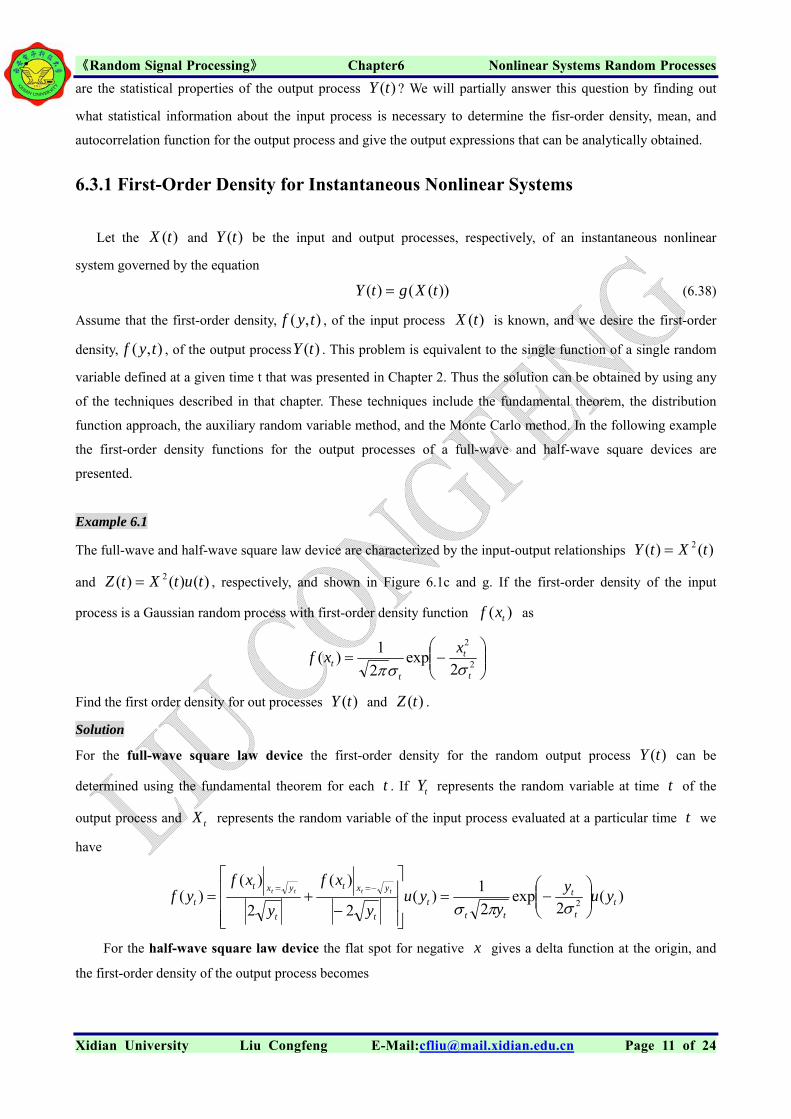
Solution

By method 1 the autocorrelation function of the output is calculated directly in terms of the input second-order

density using

212122

21

22

2121 ,),(

21dxdxxxfxxXXEttR XXYY

Since is a Gaussian random process, the random variables )(tX 11)( XtX and are jointly

Gaussian. Thus the formula above for the autocorrelation is the fourth-order moment determined in Example 2.28.

Recall that it is given by

22 )( XtX

212

22

21

22

21 1 XXE

Where

000

0,

)0(0,

)0(0,

212/12/1

21

21

212112

22222

222

11122

121

XX

XX

XXXX

XX

XXXX

XXXX

R

ttR

RR

ttRXEXEXXE

RttRXEXE

RttRXEXE

Substituting the expressions above for and 22

21 , 12 into the fourth-order moment equation gives the output

correlation function as

)()0()0())0(

)(1)(0(),( 21

221221

2 ttRRRR

ttRRttR XXXXXX

XX

XXXXXX

The second-order densities for the output of a square law device were determined in Example 6.3. The

autocorrelation function of the output process can now be determined directly from that result using method 2 as

follows:

212121212121 ),;,()]()([),( dydyttyyfyytYtYEttRYY

Substituting the density function gives

212121

0 0 212121

21

,,

,,4

,

2121

2121

dydyyyfyyf

yyfyyfyy

ttR

XXXX

XXXXYY

The joint probability density function for the random variables )( 11 tXX and , defined across

the zero mean wide sense stationary process , is Gaussian with second-order density determined from (4.133)

as

)( 22 tXX

)(tX

)0()(

)()0(,

0

0,

2

1exp

2

1),;,(

21

21

2

1

12/12121

XXXX

XXXX

T

RttR

ttRRKm

x

xxwhere

mxKmxK

ttxxf

Substituting this into the equation above for ),( 21 xxf 21, ttRYY gives a very messy integral that needs to be

《Random Signal Processing》 Chapter6 Nonlinear Systems Random Processes evaluated. In this example the first method takes an easier path to finding the solution for the autocorrelation

function of the output process.

Example 6.5

It is desired to find the output autocorrelation for a hard limiter whose nonlinearity is shown in Figure 6.1d if the

input process is zero mean wide sense stationary Gaussian random process. The process is characterized by its

autocorrelation )(XXR . For the random variables )( 11 tXX and )( 22 tXX , where 21 tt its

second-order density function, in terms of the normalized autocorrelation function is known to be ),( 21 xxf

)(1

)(2exp

)(12

1),(

2221

21

21

XX

XX

XX

xxxxxxf

Where

)0(

)()(

XX

XXXX R

R

Solution

The autocorrelation function for the output of a hard limiter will be found by using Eq.(6.41):

210

0

2121

0

0 21

21

0 0

21210 0 21

212121

212121

),()1)(1(),()1)(1(

),()1)(1(),()1)(1(

),(

)]()([),(

dxdxxxfdxdxxxf

dxdxxxfdxdxxxf

dxdxxxfxgxg

tXgtXgEtYtYEttRYY

Since is a probability density function, it is known that it integrates to one as follows: ),( 21 xxf

210

0

21

0

0 2121

21

0 0

21210 0 21

),(),(

),(),(1

dxdxxxfdxdxxxf

dxdxxxfdxdxxxf

After solving this equation for the sum of the integrals in the second and fourth quadrant and substituting the

result into the equation for autocorrelation function, we have

1),(2),(2),( 21

0 0

21210 0 2121

dxdxxxfdxdxxxfttRYY

Then, replacing by in the second integral, we find it to be equal to the first integral from the symmetry of

the . So the autocorrelation becomes

1x 1x

),( 21 xxf

1),(4),( 210 0 2121

dxdxxxfttRYY

with given in the problem statement. The procedure from here is a little messy involving a change of

rectangular to polar coordinates, integration, and a change of varivales and a final integral. Details for obtaining

this integral are given in Thomas [5], where he showed the final result to be

),( 21 xxf



)0(

)(arcsin

2)(

XX

XXYY R

RR

where 21 tt .

There are several other basic approaches that can be used to solve for the autocorrelation function of the

output of instantaneous nonlinear systems. These include the characteristic function method, Price’s theorem for

Gaussian input processes, and series expansions. Thomas [5] has excellently and thoroughly developed these

techniques as well as derived formulas for the autocorrelation functions of the outputs of instantaneous nonlinear

systems to a Guassian random process input when the nonlinearity is a full-wave odd, full-wave even, and

half-wave vth law device given by . The basic techniques he explored, however, can be applied to any

type of instantaneous nonlinearity.

vxy

6.3.5 Higher-Order Moments

Let and are the input and output processes for an instantaneous nonlinear system given by

. For a square law device we see that to get the nth-order moment of the output, we must know

the input density or know the moments of the input process of order 2n. Thus a higher-order characterization of

the input process is necessary. In general, if we consider a polynomial approximation to , we need to know

all order moments of the input process to be able to determine the nth order moments of the output process.

)(tX

(tXg

)(tY

))(tY

g

6.3.6 Stationarity of Output Process

Let and be the input and output processes for an instantaneous nonlinear system given by

. We are able to make a few general statements concerning the stationarity of the output process

with respect to the stationarity of the input process.

)(tX

(tXg

)(tY

))(tY

(1) If is stationary in the mean, the output will not necessarily be stationary in the mean. )(tX

(2) If is stationary of any order n, the output process is stationary of order n. )(tX

(3) If is wide sense stationary, then is not necessarily wide sense stationary. )(tX )(tY

6.4 Characterizations for Bilinear Systems

If the input to a bilinear system is a random process , the resulting output is also a random

process. We now explore the statistical relationships that exist between input and output processes. Specifically,

we will derive the output mean and autocorrelation function, and the cross correlation between input and output

processes. Specifically, we will derive the output mean and autocorrelation function, and the cross correlation

between input and output, for a causal bilinear system represented in (6.2) by the input-output relationship.

)(tX )(tY



21210 0 212 )()(),()( ddtXtXhtY

(6.43)

Assume that ),( 212 h

),( 21 tt

is known and that is a random process characterized by its mean and

autocorrelation function, and and , respectively. The output process can be partially

characterized by its mean and autocorrelation function , Also the cross-correlation

function , between the input and output is important. These partial characterizations are determined

for the output of a bilinear system in the following sections.

)(tX

,( 21 ttYY )(tXE

)(tYE

)R )(tY

),( 21 ttRYY

RXY

6.4.1 Mean of the Output of a Bilinear System

The mean of the output process is obtained by taking the expected value and integration to give

21210 0 212 )]()([),()]([ ddtXtXEhtyE

(6.44)

The output mean can be determined only if we know the autocorrelation function of the input. Thus a higher-order

characterization of the input, other than just the mean, is required for determining the mean of the output of a

bilinear system. This is in contrast to the result for linear system, which requires only the mean of the input

process to be known to determine the mean of the output process.

If the input process is wide sense stationary with a zero mean and autocorrelation function )(XXR , then the

from (6.44) reduces to )(tYE

21210 0 212 )(),()]([ ddRhtyE XX

(6.45)

6.4.2 Cross-correlation between Input and Output of a Bilinear System

The cross correlation between the input and output process can be written as

21210 0 212

21210 0 212

)()()(),(

)()(),()()()(),(

ddtXtXtXEh

ddtXtXhtXEtYtXEttRXY

(6.46)

The cross-correlation function for the input and output of a bilinear system is thus a function of the third-order

moments of the input process. Thus, if only the second-order moments were given, we would not have been able

to determine the ),( ttRXY .

6.4.3 Autocorrelation Function for the Output of a Bilinear System

The autocorrelation function is obtained by taking the expected value of the product of the output at time and

the output at time as

1t

2t



2121221221112120 0 0 0 212

2122120 0 212

2121110 0 212

1121

)()()()(),(),(

)()(),(

)()(),(

)]()([),(

ddddtXtXtXtXEhh

ddtXtXh

ddtXtXhE

tYtYEttRYY

(6.47)

The autocorrelation function for the output of a bilinear system is thus seen to be a function of the fourth-order

moments of the input process. Clearly, a higher-order characterization of the input process—the fourth-order

moments—is needed to determine just the output autocorrelation function . ),( 21 ttRYY

6.5 Characterizations for Trilinear Systems

We now briefly look at the characteristics of the output of a trilinear system to a random input .

In particular, the mean, cross-correlation function, and autocorrelation function are presented, and we learn that

much higher-order characterizations are required to determine them.

)(tY )(tX

6.5.1 Mean of the Output of a Trilinear System

The mean of the output process of a trilinear system is obtained by taking the expected value of both sides of (6.30)

and interchanging the order of expected value and integration to give

3213213213 )]()()([),,()]([

dddtxtxtxEhtyE (6.48)

The output mean can be determined only if we know the third-order moments of the input process. Thus a

higher-order characterization of the input, other than just the mean and autocorrelation function, is required for

determining the mean of the output of a trilinear system.

6.5.2 Cross-correlation between Input and Output of a Trilinear System

The cross correlation between the input and output process can be written by multiplying (6.30) by and

taking the expected value operator through the integral signs:

)(uY

3213213213 )]()()()([),,()]()([ ddduXuXuXtXEhuYtXE

(6.49)

The cross-correlation function for the input and output of a bilinear system is a function of the fourth-order

moments of the input process.

6.5.3 Autocorrelation Function for the Output of a Trilinear System

The autocorrelation function is obtained by taking the expected value of the product of the output at time t and the


《Random Signal Processing》 Chapter6 Nonlinear Systems Random Processes output at time u as follows:

321321321321

32133213

3213213213

3213213213

)()()()()()(

),,(),,(

)()()(),,(

)]()()(),,()]()([

dddddduXuXuXtXtXtXE

hh

ddduXuXuXh

dddtXtXtXhEuYtYE

(6.50)

The autocorrelation function for the output of a trilinear system is seen to be a function of the sixth-order

moments of the input process. Thus, unless these sixth-order moments of the input are given, we would not be

able to determine the autocorrelation function for the output process of a trilinear system to a random process

input.

6.6Characterizations for Volterra Nonlinear Systems

If the input to the nonlinear system is a random process, the resulting output is a random process. We explore

here the statistical relationships that exist between input and output processes. Specifically in the following

example the output mean and autocorrelation function, and the cross correlation between input and output, will be

derived for a system represented by a truncated Volterra expansion of the second order.

Example 6.7

A nonlinear system is known to be characterized by a second-order Volterra expansion as

0 0 21212120 10 ,)( ddtxtxkdtxkktY (6.51)

Assume that ,0k 1k , and 212 , k

XE

are known and that is a random process characterized by its mean

and autocorrelation functions by and . Find (a) the mean

)(tX

))(t ,( 21 ttRXX )(tYE of the output process,

(b) the cross correlation between the input and output, and (c) the autocorrelation function of the output process.

Solution

(a) The mean of the output process is obtained by taking the expected value of both sides of (6.51) and

interchanging the order of expected value and integration to give

0 0 21212120 11110 ,)( ddtXtXEkdtXEkktYE (6.52)

The output mean can be determined only if we know both the mean of the input process and the autocorrelation

function of the input. Thus we require a higher-order characterization of the input. This is in contrast to the result

for linear systems which requires only the mean of the input process to determine the mean of the output process.

For the special case where the input process is wide sense stationary which a zero mean and autocorrelation

function )(XXR , the first integral of (6.52) is zero. The expected value in the second integral can be written in

terms of the time difference only:



0 0 21212120 )(,)( ddRkktYE XX (6.53)

(b) The cross correlation between the input and output can be written as follows using (6.51) and the

definition of the cross-correlation function as

0 0 212121210 1101

2121

,)()()(

)()(),(

ddtXtXktXdtXktXktXE

tYtXEttRXY

(6.54)

After multiplying out and taking the expected value operator through the integral sign, we reduce (6.54) to

0 0 2122121212

0 121111021

)(,

)()(),(

ddtXtXtXEk

dtXtXEktXEkttRXY (6.55)

The cross-correlation function for the input and output of a second-order Volterra system is a function of the first,

second, and third-order moments of the input process.

(c) The autocorrelation function is obtained by taking the expected value of the product of the output at time

and the output at time as follows: 1t 2t

0 0 2122122120 112110

0 0 2121112120 111110

2121

,

,

)()(),(

ddtXtXEkdtXEkk

ddtXtXEkdtXEkkE

tYtYEttRYY

(6.56)

Multiplying out the terms in parentheses it is seen that the contains nine terms and depends on the

first-through the fourth-order moments of the input process. Thus just knowing the mean and autocorrelation

function is not sufficient for determining the autocorrelation function is not sufficient for determining the

autocorrelation function of the output process.

),( 21 ttRYY

6.7 Higher-order Characterizations

We have seen that the mean, autocorrelation function, and power spectrum are sufficient for determining the

mean, autocorrelation, and power spectrum for the output of linear systems to random processes. For nonlinear

systems we have already noted that higher-order properties than the second-order statistics must be defined in

order to determine even the output statistical properties of order two. The useful definitions of moment function,

cumulant function and higher-order spectra are now presented.

6.7.1 Moment Function for Random Processes

The moment function for a random process can be considered to be an extension of the autocorrelation function.

The autocorrelation function is the expected value of the product of the random variables defined at two different

times, whereas the moment function is the expected value of the product of the random variables defined at more


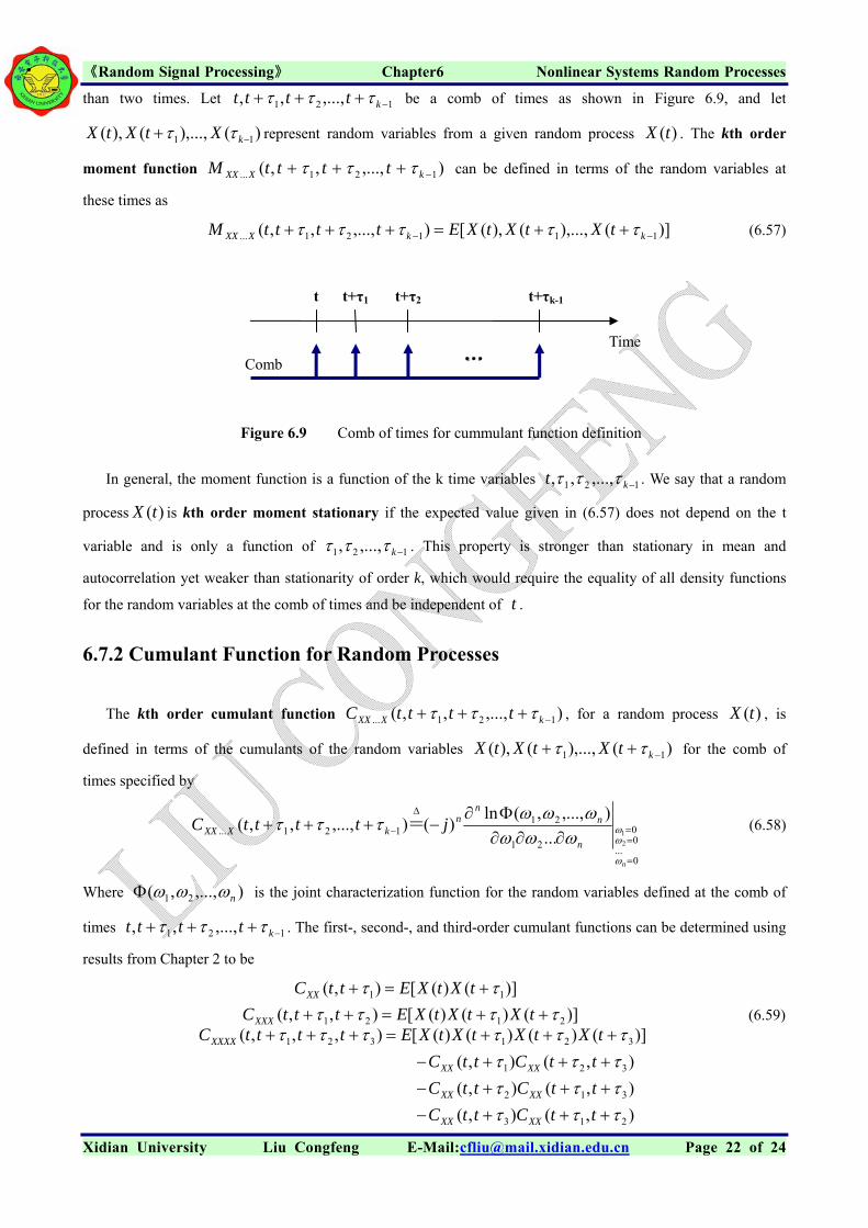
《Random Signal Processing》 Chapter6 Nonlinear Systems Random Processes than two times. Let 121 ,...,,, ktttt be a comb of times as shown in Figure 6.9, and let

)( 1k),...,(),( 1 XtXtX represent random variables from a given random process . The kth order

moment function

)(tX

)1,...,,,( 21... XXX tttt kM can be defined in terms of the random variables at

these times as

)](),...,(),([),...,,,( 11121... kkXXX tXtXtXEttttM (6.57)

t t+τ1 t+τ2 t+τk-1

Time

Comb …

Figure 6.9 Comb of times for cummulant function definition

In general, the moment function is a function of the k time variables 121 ,...,,, kt . We say that a random

process is kth order moment stationary if the expected value given in (6.57) does not depend on the t

variable and is only a function of

)(tX

121 ,...,, k . This property is stronger than stationary in mean and

autocorrelation yet weaker than stationarity of order k, which would require the equality of all density functions

for the random variables at the comb of times and be independent of . t

6.7.2 Cumulant Function for Random Processes

The kth order cumulant function ),...,,,( 121... kXXX ttttC , for a random process , is

defined in terms of the cumulants of the random variables

)(tX

)(),..., 1(),( 1 ktXtXtX for the comb of

times specified by

0...

00

21

21121...

2

1...

),...,,(ln)(),...,,,(

n

n

nn

nkXXX jttttC

＝ (6.58)

Where ),...,,( 21 n

21 ,...,,, tttt

is the joint characterization function for the random variables defined at the comb of

times 1 k . The first-, second-, and third-order cumulant functions can be determined using

results from Chapter 2 to be

),(),(

),(),(

),(),(

)]()()()([),,,()]()()([),,(

)]()([),(

213

312

321

321321

2121

11

ttCttC

ttCttC

ttCttC

tXtXtXtXEttttCtXtXtXEtttC

tXtXEttC

XXXX

XXXX

XXXX

XXXX

XXX

XX

(6.59)


《Random Signal Processing》 Chapter6 Nonlinear Systems Random Processes With the random variables defined above for the comb of times and assuming moment stationarity

of the proper order, we see that the first four cumulant functions for the process do not depend on t and

can be written as functions of the distances between the teeth of the comb as follows:

kXXX ,...,, 21

)(tX

)()(

)()(

)()(

)]()()()([),,()]()()([),(

)]()([

213

132

321

321321

2121

11

XXXX

XXXX

XXXX

XXXX

XXX

XX

CC

CC

CC

tXtXtXtXECtXtXtXEC

tXtXEC

(6.60)

6.7.3 Polyspectrum for Random Processes

The power spectral density, or power spetrum, is a partial characterization of a random process and is related

to the autocorrelation of a wide sense stationary process through the Fourier transform. In working with processes

generated as outputs from nonlinear systems, it is necessary to include higher-order characterizations. For these

problems it is useful to define the polyspectrum for a random process which is a higher-order characterization.

The kth-order polyspectrum ),...,,( 121... kXXXS of a random process , with moment stationarity

of the kth order is defined as the (k-1)-dimensional Fourier transform of its kth order cumulant function defined by

Eq.(6.58)

)(tX

Thus for and , the Tk ],...,,[ 121 T

k ],...,,[ 121 ),...,,( 121... kXXXS is defined by

djCS TXXXXXX )exp()(...)( ......

＝ (6.61)

Notice that this definition uses the Fourier transform of the cumulant function rather than the moment function.

The most commonly used polyspectra are the spectrum, bispectrum, and trispectrum. These are given as follows:

Spectrum

11111 )exp()()( djCS XXXX (6.61)

Bispectrum

2122112121 ))(exp(),(),( ddjCS XXXXXX

(6.62)

Trispectrum

321332211321321 ))(exp(),,(),,( dddjCS XXXXXXXX

(6.63)

Use of these polyspectra has led to new methods in system identification and detection algorithms. A thorough

discussion of polyspectra and the use of the cumulant spectrum is presented in Nikias and Petropuou [10], Mendel

[8], and Nikias and Mendel [6].




6.8 Summary

It is virtually impossible for our modern-day problems to not involve nonlinear systems. Therefore the main

purpose of this chapter was to present a framework for determining various characterizations of output processes

of nonlinear systems with random processes as inputs. In Chapter 5 it was shown that output mean and

autocorrelation function of a linear time-invariant system could be obtained knowing only the input mean and

autocorrelation, respectively, and that the output spectral density could be obtained in the frequency domain by

using the transfer function of the system.

It was shown in this chapter that even the simplest nonlinear system, the instantaneous nonlinear system,

requires additional statistical information other than just the mean and autocorrelation function, namely the first-

and second-order densities of the input process to determine the mean and autocorrelation function of the output

process.

A hierarchy of nonlinear systems was presented including the instantaneous nonlinear, bilinear, trilinear, and

the general Volterra system. These systems input and output relationships were described in terms of integral

equations involving various time domain kernels. This was similar to the description of a linear system in terms of

the convolution integral, but for these nonlinear systems the defining integral is represented by a higher

-dimensional integral. Analogously, frequency domain kernels were defined that could be used to obtain

higher-order spectra for the output.

The transformation theorem for random variables was the basic tool used for finding output characterizations

of instantaneous nonlinear systems to random inputs. It was used to obtain the first- and second-order density

functions and the mean and autocorrelation function of the output process. It was shown that a first-order density

of the input is required to determine just the mean of the output process and that a second-order density of the

input process is required to determine the output autocorrelation function. It was also shown that for instantaneous

nonlinear systems that an nth order stationary input process produced an nth-order stationary output process.

Solving for the output autocorrelation function was, in general, a very complex process even for Gausssian

process inputs.

The next level of nonlinearity discussed was the bilinear system. Simple bilinear systems were given as

examples and involved a linear system or systems in cascade with a square law device. It was again shown that

higher-order characterizations of the input process are required to determine just the output mean and

autocorrelation function.

Trilinear and general Volterra nonlinear systems were then presented where inputs and outputs were modeled

in terms of first-, second-, and higher-order kernels. Moment and cumulant spectra were defined and their

relationships explored.

Missing from our development is the presentation of Weiner functionals which are useful for nonlinear system

identification. Basically functionals are selected such that their outputs are orthogonal for Gaussian input

processes.

----------This is the end of Chapter06----------

Documents

Chapter 6 Nonlinear Systems Random Processes