Chapter 6: Linear Differential Equations - Penn Mathgressman/overheads_chap6.pdf · Chapter 6: Linear Di erential Equations ... Chapter 6 5/45. ... How do you know when you’ve got

Chapter 6: Linear Differential Equations

Philip Gressman

University of Pennsylvania

Philip Gressman Math 240 002 2014C: Chapter 6 1 / 45

Linear ODEs: §6.1

Definition

An n-th order linear differential equation is an equation of the form

an(x)dny

dxn+ an−1(x)

dn−1y

dxn−1+ · · ·+ a1(x)

dy

dx+ a0(x)y = g(x)

here a0(x), . . . , an(x) and g(x) are known functions, and y is(presumably) an unknown function of x .

Linear differential equations generally have more than one solution(i.e., more than one possible choice of the function y satisfies theequation). Thus there are several different ways that one mightwant to “solve” the equation.

General Solutions

The general solution of a linear differential equation is a completelisting of all possible solutions.


Initial Value Problems

If you are only care about a solution which satisfies

y(x0) = y0, y ′(x) = y1, · · · , y (n−1)(x0) = yn−1,

this is called an initial value problem. If all the coefficientfunctions aj(x) and g(x) are continuous and an never equals zeroon some interval I , then initial value problems always have exactlyone solution on that interval.

Boundary Value Problems

If you want to find solutions on some interval a ≤ x ≤ b and youhave information about the solution at both ends (for example,y(a) = y0 and y(b) = y1), this is called a boundary valueproblem. Boundary value problems are much more complicatedthan initial value problems (and may have zero, one, or manysolutions).


Notation: Differential Operators

For notational convenience, we have shorthand. If we write

L = an(x)dn

dxn+ · · ·+ a1(x)

d

dx+ a0(x)

orL = an(x)Dn + · · ·+ a1(x)D + a0(x)

Then the notation Lf is meant to refer to the function

Lf = an(x)f (n)(x) + · · ·+ a1(x)f ′(x) + a0f (x).

We call L a differential operator of order n. Linear differentialequations may always be written in shorthand Ly = g for somedifferential operator L.

Linearity

Differential operators are linear, meaning L(f + g) = Lf + Lg andL(cf ) = c(Lf ) when c is a constant.


Homogeneous Equations

Definition

The equation Ly = 0 is called homogeneous. If your equation isgiven as Ly = g for some nonzero function g , then the equationLy = 0 is called the associated homogeneous ODE.

Superposition Principle

If y1 and y2 are solutions of the homogeneous ODE Ly = 0, thenc1y1 + c2y2 will also be a solution. The same can be said for anylinear combination of any number of solutions (i.e., more than twosolutions).


Homogeneous Equations

Linear Independence

In general, we would like to avoid wasting energy on findingsolutions which can be written as a linear combination of solutionswe already know. How do you know when you’ve got “distinct”solutions? We say that functions f1, . . . , fn are linearly independenton an interval I when the only constants c1, . . . , cn such that

c1f1(x) + c2f2(x) + · · ·+ cnfn(x) ≡ 0

on the entire interval are all zeros. (Note: A previous typo has been fixed.)

Example: sin x and cos x are linearly independent on every interval.

Non-example: sin2 x , cos2 x , and 1 are linearly dependent on everyinterval.


The Wronskian

Given functions f1, . . . , fn which can be differentiated at least n− 1times, the Wronskian of f1, . . . , fn is defined to be the determinant

det

∣∣∣∣∣∣∣∣∣f1 · · · fnf ′1 · · · f ′n...

. . ....

f(n−1)

1 · · · f(n−1)n

∣∣∣∣∣∣∣∣∣ .Theorem

If f1, . . . , fn are solutions of the homogeneous ODE Ly = 0 (oforder n), then they are linearly independent solutions if and only ifthe Wronskian never equals zero. (Moreover, if it equals zerosomewhere, then it equals zero everywhere). Under theassumptions from before (the coefficients aj are continuous and annever equals zero), there will always exist a full set of n linearlyindependent solutions.


Inhomogeneous ODEs

Finding the general solution of an inhomogeneous differentialequation is only slightly more difficult than solving a homogeneousone.

1 You must first find some solution yp. It is called a particularsolution.

2 The general solution of the inhomogeneous equation willalways be of the form

y = c1y1 + · · ·+ cnyn + yp

Where y1, . . . , yn are a fundamental set of solutions (i.e., acomplete set) for the associated homogeneous differentialequation.


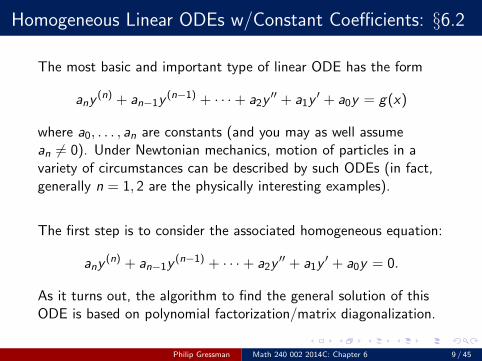
Homogeneous Linear ODEs w/Constant Coefficients: §6.2

The most basic and important type of linear ODE has the form

any(n) + an−1y

(n−1) + · · ·+ a2y′′ + a1y

′ + a0y = g(x)

where a0, . . . , an are constants (and you may as well assumean 6= 0). Under Newtonian mechanics, motion of particles in avariety of circumstances can be described by such ODEs (in fact,generally n = 1, 2 are the physically interesting examples).

The first step is to consider the associated homogeneous equation:

any(n) + an−1y

(n−1) + · · ·+ a2y′′ + a1y

′ + a0y = 0.

As it turns out, the algorithm to find the general solution of thisODE is based on polynomial factorization/matrix diagonalization.


Homogeneous Linear ODEs w/Constant Coefficients

Using our notation: Consider the linear ODE

any(n) + an−1y

(n−1) + · · ·+ a2y′′ + a1y

′ + a0y = 0.

and the polynomial

p(t) := antn + · · ·+ a1t + a0.

In our linear differential operator notation,

any(n) + an−1y

(n−1) + · · ·+ a2y′′+ a1y

′+ a0y = 0⇔ p (Dx) y = 0.

But polynomials always factor over the complex numbers:

p(t) = an(t − t1)m1 · · · (t − tk)mk

where t1, . . . , tk are the distinct roots and m1, . . . ,mk are theirmultiplicities. We know k ≤ n and m1 + · · ·+ mk = n.



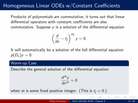
Products of polynomials are commutative; it turns out that lineardifferential operators with constant coefficients are alsocommutative. Suppose y is a solution of the differential equation(

d

dx− tj

)mj

y = 0.

It will automatically be a solution of the full differential equationp(Dx)y = 0.

Warm-up Case

Describe the general solution of the differential equation

dmy

dxm= 0

when m is some fixed positive integer. (This is tj = 0.)



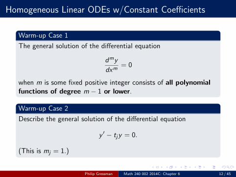
Warm-up Case 1

The general solution of the differential equation

dmy

dxm= 0

when m is some fixed positive integer consists of all polynomialfunctions of degree m − 1 or lower.

Warm-up Case 2

Describe the general solution of the differential equation

y ′ − tjy = 0.

(This is mj = 1.)


Warm-up Case 2

The general solution of the differential equation

y ′ − tjy = 0

has the form y = etjx .

Notice the similarity to the eigenvector equation. We call etjx aneigenfunction of the operator d

dx with eigenvalue tj .

About Complex Roots/Eigenvalues

You can use Euler’s formula:

e i = cos + i sin.

For example:

e(3+2i)t = e3t cos 2t + e3t i sin 2t.


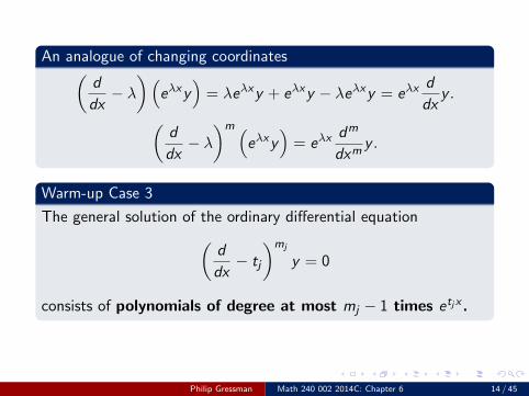
An analogue of changing coordinates(d

dx− λ

)(eλxy

)= λeλxy + eλxy − λeλxy = eλx

d

dxy .(

d

dx− λ

)m (eλxy

)= eλx

dm

dxmy .

Warm-up Case 3

The general solution of the ordinary differential equation(d

dx− tj

)mj

y = 0

consists of polynomials of degree at most mj − 1 times etjx .


General Solution of any(n) + · · ·+ a1y

′ + a0y = 0.

• Step 1: Find all solutions to the auxiliary equation

anλn + · · ·+ a1λ+ a0 = 0

and make note of their multiplicities.

• Step 2: For each root λj , if the multiplicity is mj , then therewill be solutions

c0eλjx + · · ·+ cmj−1x

mj−1eλjx .

• Step 3: The general solution will be a linear combination ofall such solutions for all possible λj . If there were complexroots, simplify into cos and sin with Euler’s formula. If therewere no complex numbers in the original statement, itwill always be possible to simplify to the point that thereare no complex numbers in the solution!!!

• Step 4: If you’ve got an IVP, solve for the appropriatecoefficients.


Inhomogeneous Eqns: Method of Undetermined Coeffs.

Objective

Find the general solution of the inhomogeneous ODE

anDny + · · ·+ a1Dy + a0y = g(x).

We only need to find a single solution, then we can infer the rest ofthe solutions by studying the homogeneous problem. When g hasa certain form, it’s possible to guess the form of the answer, putcoefficients in front of each terms and try to solve for thecoefficients.In other words, we restrict our attention to a well-chosen,finite-dimensional subspace of functions, then turn the probleminto a finite linear algebra problem.• Good idea for: polynomials, exponentials, sines, cosines, and

products of functions of this form.• Bad idea for: most other functions which are more

complicated than this.Philip Gressman Math 240 002 2014C: Chapter 6 16 / 45

Undetermined Coefficients

Example:y ′′ − 2y ′ + 2y = 4.

• We hope that there is a “simple” particular solution to thisODE. An example of something simple is a constant solution.

• Plug in y = A, we get

(A)′′ − 2(A)′ + 2(A) = 4⇒ 2A = 4⇒ A = 2.

• Not all guesses produce solutions: If we wanted a solution ofthe form y = Ax , we have

(Ax)′′ − 2(Ax)′ + 2(Ax) = 4⇒ 0− 2A + 2Ax = 4.

There is no one value of A which solves the equation for allvalues of x .


Undetermined Coefficients

Example:y ′′ + 2y ′ + y = ex + 5e2x .

We might guess that there is a solution to this equation whichbelongs to the span of ex and e2x . So we would takeyp = Aex + Be2x , substitute, and solve. We get yp = 1

4ex + 5

9e2x .

Helpful Fact #1

IfL(D)y = g1(x) + g2(x)

we can solve the equations L(D)y = g1(x) and L(D)y = g2(x) andthen add the two separate particular solutions together at the end(saves work).


Comments on Undetermined Coefficients

• To find a solution, you must be able to solve for constantswhich work simultaneously for all values of x .

• If your right-hand side is a sum of multiple terms, just makeguesses for each individual term. BUT there’s no point inmaking a guess which has terms like Aex + Bex + · · · . Eachkind of term in your guess should appear only once.

• There’s no harm in including many terms in your guess, but itdoes make more work to solve.

• The method needs to be modified in the presence ofresonance terms. A resonance term on the right-hand side isone which is actually a solution of the associatedhomogeneous ODE.


Helpful Approach: AnnihilatorsFor any given function g , we say that a differential operator P(D)annihilates f if P(D)g = 0.

(D − λ) annihilates eλx

(D − λ)k annihilates eλx , . . . , xk−1eλx

(D2 − 2aD + (a2 + b2)) annihilates eax cos bx , eax sin bx

(D2 − 2aD + (a2 + b2))k annihilates eax cos bx , eax sin bx ,

xeax cos bx , xeax sin bx ,

...

xk−1eax cos bx ,

xk−1eax sin bx

Above λ could be real or complex. Both a and b must be real andb must not equal zero. If you can find the annihilator of theright-hand side of an ODE, apply it to both sides and you’ll get ahomogeneous ODE instead.


Helpful Approach: Complex-valued Trial Solutions

When the inhomogeneous part has sines and cosines, there are afew tricks you can sometimes use to make life easier.

• Use Euler’s formula:

sin θ =e iθ − e−iθ

2icos θ =

e iθ + e−iθ

2

If you substitute this in for sine and cosine, you’ll double thenumber of terms, but each term will have a simplerannihilator (often the trade-off) is worth it.

• If all coefficients are real You can also use the fact thatcos θ is the real part of e iθ and sin θ is its imaginary parts.The point is that if the coefficients are all real, then the realpart of any solution is a solution and the imaginary part ofany solution is a different solution.


Resonances

The method of Undetermined Coefficients requires especiallyeducated guesses when the driving term (i.e., the right-hand side)includes functions which are solutions of the homogeneous ODE.Consider the example

y ′′ + y = 2 cos x .

Here’s a particular solution:


Resonances

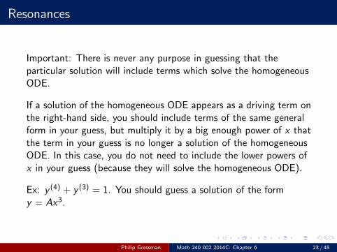
Important: There is never any purpose in guessing that theparticular solution will include terms which solve the homogeneousODE.

If a solution of the homogeneous ODE appears as a driving term onthe right-hand side, you should include terms of the same generalform in your guess, but multiply it by a big enough power of x thatthe term in your guess is no longer a solution of the homogeneousODE. In this case, you do not need to include the lower powers ofx in your guess (because they will solve the homogeneous ODE).

Ex: y (4) + y (3) = 1. You should guess a solution of the formy = Ax3.


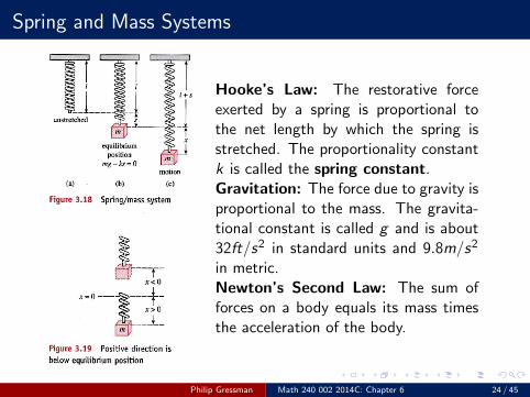
Spring and Mass Systems

Hooke’s Law: The restorative forceexerted by a spring is proportional tothe net length by which the spring isstretched. The proportionality constantk is called the spring constant.Gravitation: The force due to gravity isproportional to the mass. The gravita-tional constant is called g and is about32ft/s2 in standard units and 9.8m/s2

in metric.Newton’s Second Law: The sum offorces on a body equals its mass timesthe acceleration of the body.


Free Undamped Motion

The simplest scenario takes into account only gravity and thespring. This is called free, undamped motion. Free means thatthere is no outside driving force and undamped means there is nofriction/wind resistance/viscous forces/etc.

The Free Undamped Oscillator

The equation of a free undamped oscillator has the form

md2x

dt2+ kx = 0.

Both m and k are positive. Let ω :=√

km . The general solution

may be written as either

x(t) = c1 cosωt + c2 sinωt,

x(t) = A cos(ωt − φ).


Simple Harmonic Motion or Free Undamped Motion

md2x

dt2+ kx = 0.

There’s lots of terminology:

• ω :=√

km is called the angular frequency.

• f := ω2π is called the frequency. It equals the number of

complete cycles which occur in one unit time.

• T := 1f is the period—the time necessary for one full cycle.

x(t) = c1 cosωt + c2 sinωt,

x(t) = A cos(ωt − φ).

• A is called the amplitude.

• φ is called the phase angle.

Conversions between the two forms of general solution requiretrigonometry and trig identities.


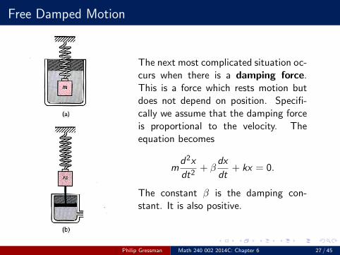
Free Damped Motion

The next most complicated situation oc-curs when there is a damping force.This is a force which rests motion butdoes not depend on position. Specifi-cally we assume that the damping forceis proportional to the velocity. Theequation becomes

md2x

dt2+ β

dx

dt+ kx = 0.

The constant β is the damping con-stant. It is also positive.


Free Damped Motion

md2x

dt2+ β

dx

dt+ kx = 0.

The auxiliary equation has roots

−β ±√β2 − 4mk

2m.

We split into three cases:

• β2 − 4mk < 0: This case is called underdamped.

• β2 − 4mk = 0: This is critically damped.

• β2 − 4mk > 0: This is called overdamped.


Underdamped Motion

Free Damped Motion

md2x

dt2+ β

dx

dt+ kx = 0.

β2 − 4mk < 0: Underdamped. General solution has form

c1e− β

2mt cos

(√4mk − β2

2mt

)+ c2e

− β2m

t sin

(√4mk − β2

2mt

)or

Ae−β

2mt cos

(√4mk − β2

2mt − φ

)The graph is a sine wave with exponentially decaying amplitude.As β gets closer and closer to

√4mk , the exponential rate of decay

increases and the period of oscillation increases without limit.


Critically Damped Motion

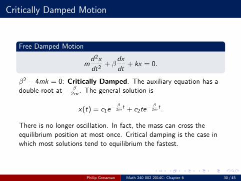
Free Damped Motion

md2x

dt2+ β

dx

dt+ kx = 0.

β2 − 4mk = 0: Critically Damped. The auxiliary equation has adouble root at − β

2m . The general solution is

x(t) = c1e− β

2mt + c2te

− β2m

t .

There is no longer oscillation. In fact, the mass can cross theequilibrium position at most once. Critical damping is the case inwhich most solutions tend to equilibrium the fastest.


Overamped Motion

Free Damped Motion

md2x

dt2+ β

dx

dt+ kx = 0.

β2 − 4mk > 0: Overdamped. The auxiliary equation has twonegative real roots. The general solution is

x(t) = c1e(− β

2m+

√β2−4mk

2m)t + c2e

(− β2m−√

β2−4mk2m

)t .

There is no oscillation. One of the two exponentials decays fasterthan the critically damped, but the other decays more slowly.


Driving Forces

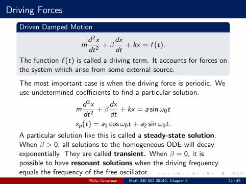
Driven Damped Motion

md2x

dt2+ β

dx

dt+ kx = f (t).

The function f (t) is called a driving term. It accounts for forces onthe system which arise from some external source.

The most important case is when the driving force is periodic. Weuse undetermined coefficients to find a particular solution.

md2x

dt2+ β

dx

dt+ kx = a sinω0t

xp(t) = a1 cosω0t + a2 sinω0t.

A particular solution like this is called a steady-state solution.When β > 0, all solutions to the homogeneous ODE will decayexponentially. They are called transient. When β = 0, it ispossible to have resonant solutions when the driving frequencyequals the frequency of the free oscillator.


Electrical Analogue

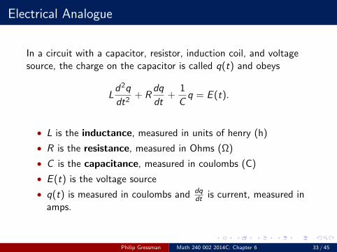
In a circuit with a capacitor, resistor, induction coil, and voltagesource, the charge on the capacitor is called q(t) and obeys

Ld2q

dt2+ R

dq

dt+

1

Cq = E (t).

• L is the inductance, measured in units of henry (h)

• R is the resistance, measured in Ohms (Ω)

• C is the capacitance, measured in coulombs (C)

• E (t) is the voltage source

• q(t) is measured in coulombs and dqdt is current, measured in

amps.


Variation of Parameters

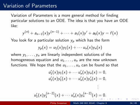
Variation of Parameters is a more general method for findingparticular solutions to an ODE. The idea is that you have an ODElike:

y (n) + an−1(x)y (n−1) + · · ·+ a1(x)y ′ + a0(x)y = f (x)

You look for a particular solution yp which has the form

yp(x) = u1(x)y1(x) + · · · un(x)yn(x)

where y1, . . . , yn are linearly independent solutions of thehomogeneous equation and u1, . . . , un are the new unknownfunctions. We hope that the u1, . . . , un can be found so that

u′1(x)y1(x) + · · · u′n(x)yn(x) = 0,

u′1(x)y ′1(x) + · · · u′n(x)y ′n(x) = 0,

...

u′1(x)y(n−2)1 (x) + · · · u′n(x)y

(n−2)n (x) = 0.


Variation of Parameters

Example 1

y ′′ + 2y ′ + y = ex

Example 2

y ′′ − 2y ′ + y =ex

x2 + 1

Example 3

xy ′′ − (x + 1)y ′ + y = x2

(Note: ex and x + 1 solve the homogeneous ODE.)


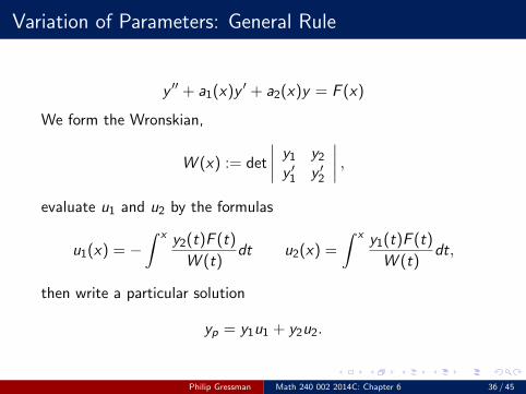
Variation of Parameters: General Rule

y ′′ + a1(x)y ′ + a2(x)y = F (x)

We form the Wronskian,

W (x) := det

∣∣∣∣ y1 y2

y ′1 y ′2

∣∣∣∣ ,evaluate u1 and u2 by the formulas

u1(x) = −∫ x y2(t)F (t)

W (t)dt u2(x) =

∫ x y1(t)F (t)

W (t)dt,

then write a particular solution

yp = y1u1 + y2u2.


Cauchy-Euler Equations

Cauchy-Euler Equations (sometimes called equidimensionalequations) are the simplest examples of linear ODEs whosecoefficients are not constant. The general form of such anequation has the form

anxny (n) + an−1x

n−1y (n−1) + · · ·+ a1xy′ + a0y = g(x).

Here an, . . . , a0 are constants. Notice that the power of x alwaysmatches the number of derivatives on the unknown function y ineach term.There are two distinct methods which are useful when solving thistype of equation:

• The direct approach: Various rules to learn for solving thesekinds of equations.

• Substitution: Convert this kind of equation to a constantcoefficient one.


Cauchy-Euler: The Direct Approach

Much like with constant coefficients, this method is based onbuilding blocks that you combine to form a general solution.Unlike exponential functions, this time we use powers: y = xm.IMPORTANT: We might take m to be a complicated number oreven complex if the situation warrants.

The Fundamental Identity

xd

dx[xm] = mxm

x2 d2

dx2[xm] = m(m − 1)xm

...

xkdk

dxk[xm] = m(m − 1) · · · (m − k + 1)xm.


Cauchy-Euler: The Direct Approach

The auxiliary equation for a Cauchy-Euler equation is constructedby assuming y = xm, plugging in, and collecting coefficients:Example:

x2y ′′ + 2xy ′ + y = 0⇒ m(m − 1) + 2m + 1 = 0.

As with constant coefficient equations, you solve for m. There willbe complications when there are complex roots and when there arerepeated roots.


The Direct Approach Algorithm

• Step 1: Write down and solve the auxiliary equation.

• Step 2: Solutions which are real and have multiplicity one justcorrespond to terms in the general solution which are powersof x :

m = 1.1 with multiplicity 1⇒ term of the form Cx1.1.

• Step 2: Terms which are complex simplify much the same waythat they did for constant coefficients.

Cx1+3i + C ′x1−3i ; Ax cos ln 3x + Bx sin ln 3x .

• Step 3: Terms with repeated roots get multiplied by powers ofln x .

m = 1.1 w/ multiplicity 3⇒ C1x1.1+C2x

1.1 ln x+C3x1.1(ln x)2.


Cauchy-Euler: Substitution

The alternate approach is to make the substitution x = et . Youcan convert by means of the chain rule:

dy

dt=

dy

dx

dx

dt= x

dy

dxd2y

dt2= x

dy

dx+ x2 d

2y

d2xd3y

dt2= x

dy

dx+ 3x2 d

2y

dx2+ x3 d

3y

dx3

...


Aside: Integrating Factors (§1.6)

For a first-order ODE of the form

a(x)y ′ + b(x)y = c(x)

often the left-hand side can be written as the derivative ofa(x)y(x). What condition on b(x) would make this hypothesistrue? If this were true, the equation could be solved by simplyintegrating both sides (be sure to keep track of integrationconstants).When the integration trick doesn’t work, it’s always possible tomultiply the whole equation by an integrating factor I (x) whichmakes the above trick work. That is, for

I (x)a(x)y ′ + I (x)b(x)y = I (x)c(x),

when will the left hand side equal (I (x)a(x)y)′? This can alwaysbe forced to be true by you, the solver, if you choose I correctly.


Integrating Factors: The Key Observation

For the ODE

y ′ +b(x)

a(x)y =

c(x)

a(x)

the integrating factor I (x) should satisfy I ′(x) = b(x)a(x) I (x), or

I ′

I = b(x)a(x) . This has a solution

I (x) = e∫ x b(t)

a(t)dt

giving

y =1

I (x)

∫ x c(t)

a(t)I (t)dt.

But don’t bother to memorize this formula. Memorize the processinstead, because it’s short and it’s far more useful than just havingthe formula. Example:

y ′ + xy = x .


Reduction of Order: §6.9

If you know one solution y1 to a homogeneous ODE, you can makea substitution y = uy1 and then solve for u instead of y . Theadvantage is that there will be no u terms, only u′ and higher.This means that if you solve for u′, it will be an ODE of lowerorder. If the equation is initially second-order, then solving for u′

will involve a first-order equation, which can generally be solvedusing integrating factors.Examples:

x2y ′′ − 3xy ′ + 4y = 0, y1(x) = x2

xy ′′ + (1− 2x)y ′ + (x − 1)y = 0, y1(x) = ex

y ′′ − 4y ′ + 4y = 4e2x ln x = 0, y1(x) = e2x

(1− x2)y ′′ − 2xy ′ + 2y = 0, y1(x) = x


Bonus Round: How would you solve these equations?

y ′′ + y = 3ex

x2y ′′ +1

4y = x−

12

y ′′ + y = cos x

y ′′ + y =1

sin xy ′′ + xy ′ = x3

y ′′′ + 2y ′′ + y ′ = x


Documents

Chapter 6: Linear Differential Equations - Penn Mathgressman/overheads_chap6.pdf · Chapter 6: Linear Di erential Equations ... Chapter 6 5/45. ... How do you know when you’ve got