Chapter 6. HorticultureAdapting the horticultural and vegetable industries to climate change

Brent Clothier Plant & Food ResearchAlistair Hall Plant & Food ResearchSteve Green Plant & Food Research

AbstractHorticulture is a NZ$6 billion industry for New Zealand, and exports from wine, kiwifruit and apples generate NZ$3.4 billion of export revenues. These export receipts are realised from just 55,000 ha of land, with the major concentrations of grape growing being in Marlborough, kiwifruit in the Bay of Plenty, and apple growing in Hawke’s Bay. The impacts of future climate change have been assessed for these three major export sectors, and consideration is given to how, through adaptation, these industries can overcome the challenge of climate change. Some specific impacts and adaptations for the domestic vegetable production sector are also considered. The impacts of climate change for horticulture were modelled using SPASMO (the Soil Plant Atmosphere System Model), a mechanistic model of crop growth for the three perennial horticultural crops. Tactical adaptations will include increased pruning requirements and more overhead netting will probably be required to mitigate higher temperatures. New cultivars are currently introduced regularly in all horticultural industries, so the future strategic issue will be selection of varieties appropriate for each region in a changing climate. New irrigation schemes are being developed through the Government’s Irrigation Acceleration Fund, and these are likely to benefit horticulture. Expansion into new regions will occur as innovative growers and industries see transformational possibilities for growing new crops and new cultivars in new regions. The horticultural industry, especially viticulture, is nimble, and it has already shown that it can undergo transformational change in response to economic opportunities. If the transformational change of seeking new regions in which to grow existing crops is brought about by climate change, then it is likely this transformation will occur – competition for land and water notwithstanding.

Contents1 Introduction 2412 Impacts on horticulture 242

2.1 Temperature 2432.1.1 Averages 2432.1.2 Frosts 2452.1.3 Extreme high temperature 246

2.2 Carbon dioxide 2462.3 Rainfall 2472.4 Extreme events 248

3 Horticultural adaptation 2503.1 Adaptive capacity 250

3.1.1 Tactical adaptation 2543.1.2 Strategic adaptation 2553.1.3 Transformational adaptation 255

3.2 Adaptation summary 256

4 Integrated adaptation analysis 2564.1 The SPASMO modelling framework 257

4.1.1 Biomass response 2574.1.2 Development response 2574.1.3 Quality and yield response 258

4.2 Horticulture system indicators 2604.2.1 Base level impacts 2614.2.2 Biomass and yield 261

4.2.2.1 Quality 2644.3 Effects of adaptations 265

4.3.1 Tactical 2654.3.1.1 Irrigation 265

4.3.2 Strategic 2684.3.2.1 Extreme events 268

4.3.3 Transformational adaptation 2724.4 Evaluation of productivity and profitability 272

4.4.1 Tactical 2724.4.2 Strategic 2734.4.3 Transformational 273

4.5 Knowledge gaps 273

5 Summary 2746 References 2747 Appendix A 2778 Appendix B 289

241

1 Introduction

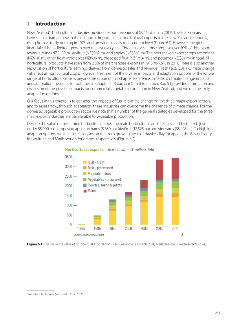
New Zealand’s horticultural industries provided export revenues of $3.46 billion in 20111. The last 35 years have seen a dramatic rise in the economic importance of horticultural exports to the New Zealand economy, rising from virtually nothing in 1975, and growing steadily to its current level (Figure 6.1). However, the global financial crisis has limited growth over the last two years. Three major sectors comprise over 70% of this export revenue: wine (NZ$1.09 b), kiwifruit (NZ$962 m), and apples (NZ$363 m). The next-ranked export crops are onions (NZ$110 m), other fresh vegetables NZ($96 m), processed fruit (NZ$79.4 m), and potatoes NZ($81 m). In total, all horticultural products, have risen from 2.0% of merchandise exports in 1975, to 7.5% in 2011. There is also another NZ$3 billion of horticultural earnings derived from domestic sales and revenue (Fresh Facts 2011). Climate change will affect all horticultural crops. However, treatment of the diverse impacts and adaptation options of the whole range of horticultural crops is beyond the scope of this chapter. Reference is made to climate-change impacts and adaptation measures for potatoes in Chapter 5 (Broad acre). In this chapter, Box 6.1 provides information and discussion of the possible impacts for commercial vegetable production in New Zealand, and we outline likely adaptation options.

Our focus in this chapter is to consider the impacts of future climate change on the three major export sectors, and to assess how, through adaptation, these industries can overcome the challenge of climate change. For the domestic vegetable production sector we note that a number of the general strategies developed for the three main export industries are transferable to vegetable production.

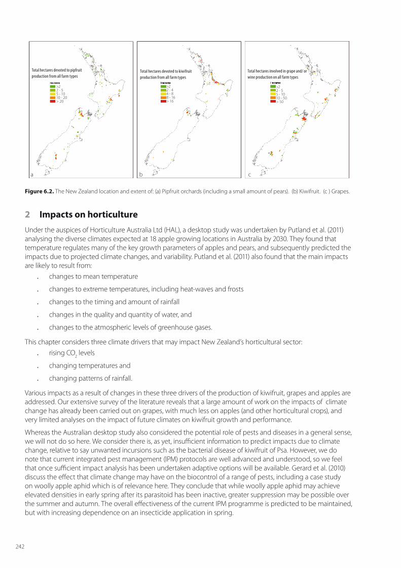
Despite the value of these three horticultural crops, the main horticultural land area covered by them is just under 55,000 ha, comprising apple orchards (8,630 ha), kiwifruit (12,525 ha) and vineyards (33,428 ha). To highlight adaption options, we focus our analyses on the main growing areas of Hawke’s Bay for apples, the Bay of Plenty for kiwifruit, and Marlborough for grapes, respectively (Figure 6.2).

Figure 6.1. The rise in the value of horticultural exports from New Zealand (Fresh Facts 2011, available from www.freshfacts.co.nz).

1www.freshfacts.co.nz (accessed 8 April 2012).

242

Figure 6.2. The New Zealand location and extent of: (a) Pipfruit orchards (including a small amount of pears). (b) Kiwifruit. (c ) Grapes.

2 Impacts on horticulture

Under the auspices of Horticulture Australia Ltd (HAL), a desktop study was undertaken by Putland et al. (2011) analysing the diverse climates expected at 18 apple growing locations in Australia by 2030. They found that temperature regulates many of the key growth parameters of apples and pears, and subsequently predicted the impacts due to projected climate changes, and variability. Putland et al. (2011) also found that the main impacts are likely to result from:

. changes to mean temperature

. changes to extreme temperatures, including heat-waves and frosts

. changes to the timing and amount of rainfall

. changes in the quality and quantity of water, and

. changes to the atmospheric levels of greenhouse gases.

This chapter considers three climate drivers that may impact New Zealand’s horticultural sector: . rising CO2 levels

. changing temperatures and

. changing patterns of rainfall.

Various impacts as a result of changes in these three drivers of the production of kiwifruit, grapes and apples are addressed. Our extensive survey of the literature reveals that a large amount of work on the impacts of climate change has already been carried out on grapes, with much less on apples (and other horticultural crops), and very limited analyses on the impact of future climates on kiwifruit growth and performance.

Whereas the Australian desktop study also considered the potential role of pests and diseases in a general sense, we will not do so here. We consider there is, as yet, insufficient information to predict impacts due to climate change, relative to say unwanted incursions such as the bacterial disease of kiwifruit of Psa. However, we do note that current integrated pest management (IPM) protocols are well advanced and understood, so we feel that once sufficient impact analysis has been undertaken adaptive options will be available. Gerard et al. (2010) discuss the effect that climate change may have on the biocontrol of a range of pests, including a case study on woolly apple aphid which is of relevance here. They conclude that while woolly apple aphid may achieve elevated densities in early spring after its parasitoid has been inactive, greater suppression may be possible over the summer and autumn. The overall effectiveness of the current IPM programme is predicted to be maintained, but with increasing dependence on an insecticide application in spring.

a b c

Total hectares devoted to pipfruit production from all farm types

Total hectares devoted to kiwifruit production from all farm types

>22 - 55 - 1010 - 20> 20

>22 - 44 - 88 - 16> 16

>22 - 55 - 1010 - 50> 50

Total hectares involved in grape and/ or wine production on all farm types

243

Kenny (2008) summarised our current knowledge of climate change as applied to New Zealand’s kiwifruit, identifying expected warming trends and associated changes in precipitation changes in current growing regions. Expected changes in extreme events were identified. A major focus of Kenny’s (2008) work was to elucidate growers’ understanding of, and response to, climate change and variability. He found that there was an increasing awareness by growers of climate change and its possible impact on their business. The main concerns were the potential for increased frequency of extreme weather events, and the effects that warmer temperatures and changed precipitation patterns might have on pests and diseases. Kenny (2008) found that the capacity of growers to adapt is high, with growers already demonstrating a willingness and ability to try different management systems in response to challenges. There was a confidence that growers and the industry as a whole have the capacity to adapt to a progressive warming of the climate, although this was balanced somewhat by the perceived potential for increased frequency of extreme events. Support for relevant research was highlighted. This chapter provides that underpinning research, and we will use these results in a programme of consultation with growers and the industries.

2.1 Temperature

Under generally accepted climate change scenarios, the overall expectation is for average temperatures to continue to rise across New Zealand, with subsequent increases in the probability of high-temperature days, reductions in the number of frosts and shifts in the diurnal temperature range (Chapter 2) The impacts related to temperature are many and diverse, and can be broken down into those that affect:

. winter chilling

. flowering and bud burst

. harvest date and yield

. fruit and wine quality

. extreme high temperatures

. frost and hail.

Temperature has a multitude of effects on horticultural crops, and is considered the source of the major impacts on horticultural production. The information for, and understanding of, how temperature affects horticultural production is variable by impact category, and it varies with crop type. In this chapter, these impacts are first reviewed and then followed by modelling to assess the impacts of future climate change. We conclude by an assessment of net benefits of specific adaptation measures

2.1.1 Averages

Deciduous fruit trees and vines require a certain amount of accumulated chilling, or vernalisation to break winter dormancy. Inadequate chilling, a prospect with future climate change, may result in prolonged dormancy, which will result in poorer fruit quality, lower yield, and potentially higher costs. nternational studies indicate that deciduous fruit trees and vines do require a certain amount of chilling to break winter dormancy. Whilst limited work has been carried out in New Zealand on the winter chilling of grapes and apples, there have been many analyses of the winter chilling requirements of kiwifruit.

In Australia, there have been several studies on winter chilling for apples. Hennessey and Clayton-Greene (1995) suggested that (by 2030) for a high warming climate-change scenario there would be a risk of prolonged dormancy at many sites. Darbyshire et al. (2011) used four chilling models to better unravel the needs for winter chilling across Australia’s major apple growing regions. Putland et al (2011) noted that most Australian apple cultivars have chill requirements of between 500 and 1000 hours per year. Apple growing regions in Western Australia, Queensland and Victoria were vulnerable, and one adaptation mooted in Australia is to grow cultivars having lower chill needs (such as cultivars grown in Florida which have chill needs of around just 250 hours). They also found that in the colder apple growing regions of Tasmania and New South Wales, a small amount of warming could actually increase winter chilling, as winter chilling is found to be best in the range between 0°C and 7.2°C.

244

Current practice in In New Zealand is to undertake both chemical and hand thinning of flowers (at least with apples) because of excessive flowering. With future warming, there might be a reduced need to thin the excessive flower numbers – and this would probably represent a cost saving. In New Zealand, Kenny (2001) noted that there would be positives and negatives of warmer temperatures for apples as ‘…the weather pattern associated with the 1997/98 El Niño event contributed to larger apple sizes, but sunburn and water-core damage resulted in significant crop losses.’

There have been a few studies on the winter chill needs of grapes, and the impact of treatments such as hydrogen cyanamide on securing the release of grapevine buds from dormancy (Shulman et al. 1983). Because we have no New Zealand information appropriate for grapes and apples, we will not consider the impact of climate change on flower numbers for grapes. Trought’s (2005) ‘yield model’ does consider a ‘bunch number’ component that can be interpreted as the number of inflorescences. This number is mainly dependent on temperatures at initiation during the previous spring. Plant & Food Research also holds bunch number data to complement phenology data, and this chapter more thoroughly examines that data set. However, understanding and unravelling wine grape yield data is complex because it is also both management- and plant-reserves dependent. Plant & Food Research also has flower number data for apples, although this may not be very relevant as flower thinning by chemical means is usual.

The phenology of fruit trees and vines is strongly dependent on the seasonal pattern of temperature. The key dates in the phenological cycle are bud break, flowering, and veraison for grapes; and harvest date which is determined by the appropriate ripeness of the fruit, or berry. Summer temperatures affect tree crops and vine crops differently. In tree crops such as apple, increased temperatures lead increased fruit growth (Austin et al. 1999), but in vine crops such as grapes or kiwifruit, increased temperatures tend to favour vegetative over reproductive development, and very high summer temperatures can lead to small, low Brix fruit (Richardson et al. 2004).

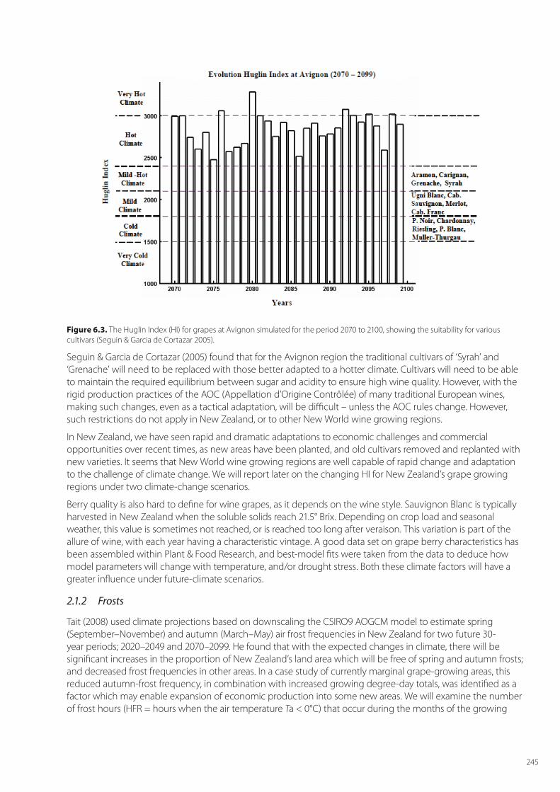
Seguin & Garcia de Cortazar (2005) note that for grapes the most important impact of climate change will come through the impact of seasonal temperatures on grape phenology, and that rising temperatures will lead to changes in the suitability of cultivars for any region. A metric of the impact of seasonal temperature is the Huglin index (HI) which, for the Northern Hemisphere, is calculated from 01 April 1 to 30 September. This index enables different viticultural regions of the world to be classified in terms of the sum of temperatures required for vine development and grape ripening (Huglin, 1978). Specifically, it is the sum of mean and maximum temperatures above +10°C (the thermal threshold for vine development). Different grape varieties are classified according to their minimal thermal requirement for grape ripening. For example, the HI is 1700 for Merlot and 2100 for Syrah (Figure 6.3). The minimal HI for vine development is 1500. 

245

Figure 6.3. The Huglin Index (HI) for grapes at Avignon simulated for the period 2070 to 2100, showing the suitability for various cultivars (Seguin & Garcia de Cortazar 2005).

Seguin & Garcia de Cortazar (2005) found that for the Avignon region the traditional cultivars of ‘Syrah’ and ‘Grenache’ will need to be replaced with those better adapted to a hotter climate. Cultivars will need to be able to maintain the required equilibrium between sugar and acidity to ensure high wine quality. However, with the rigid production practices of the AOC (Appellation d’Origine Contrôlée) of many traditional European wines, making such changes, even as a tactical adaptation, will be difficult – unless the AOC rules change. However, such restrictions do not apply in New Zealand, or to other New World wine growing regions.

In New Zealand, we have seen rapid and dramatic adaptations to economic challenges and commercial opportunities over recent times, as new areas have been planted, and old cultivars removed and replanted with new varieties. It seems that New World wine growing regions are well capable of rapid change and adaptation to the challenge of climate change. We will report later on the changing HI for New Zealand’s grape growing regions under two climate-change scenarios.

Berry quality is also hard to define for wine grapes, as it depends on the wine style. Sauvignon Blanc is typically harvested in New Zealand when the soluble solids reach 21.5° Brix. Depending on crop load and seasonal weather, this value is sometimes not reached, or is reached too long after veraison. This variation is part of the allure of wine, with each year having a characteristic vintage. A good data set on grape berry characteristics has been assembled within Plant & Food Research, and best-model fits were taken from the data to deduce how model parameters will change with temperature, and/or drought stress. Both these climate factors will have a greater influence under future-climate scenarios.

2.1.2 Frosts

Tait (2008) used climate projections based on downscaling the CSIRO9 AOGCM model to estimate spring (September–November) and autumn (March–May) air frost frequencies in New Zealand for two future 30-year periods; 2020–2049 and 2070–2099. He found that with the expected changes in climate, there will be significant increases in the proportion of New Zealand’s land area which will be free of spring and autumn frosts; and decreased frost frequencies in other areas. In a case study of currently marginal grape-growing areas, this reduced autumn-frost frequency, in combination with increased growing degree-day totals, was identified as a factor which may enable expansion of economic production into some new areas. We will examine the number of frost hours (HFR = hours when the air temperature Ta < 0°C) that occur during the months of the growing

246

season under our two high and low IPCC scenarios of climate change. The number of hours of frost will be used to predict the irrigation requirement for frost protection, assuming 4mm of water will be applied for every hour of frost. Our own research on grape vineyards in Marlborough has been used to tune the SPASMO (Soil Plant Atmosphere System Model) model of vineyard water use for both irrigation and frost fighting (Green 2006). The value of HFR is calculated simply using a linear interpolation between Tmax and Tmin, based on a first order heating and cooling curves. Interactions between changing frost frequencies, and the changing phenology, are then used to estimate a net effect of frost on each crop under the two climate change scenarios.

It is unlikely to be possible to assess the changing pattern of hail, however, increasingly hail netting is being used, so strategic adaptation is already being carried out.

2.1.3 Extreme high temperature

Extreme high temperatures will affect fruit quality (e.g., more sunburn on apples and kiwifruit and more ‘shrivelling’ of grapes), and have an effect on marketable yield. We will examine the number of high temperature hours (HTH = hours when Ta >32°C) that occur during the growing season under the two climate change scenarios. We will use this index to indicate the potential for fruit damage under high temperatures. Our own research on apples in Australia has recorded fruit temperatures exceeding 50°C when air temperatures rise above 32°C. The value of HTH will be calculated simply using a linear interpolation between Tmax and Tmin.

2.2 Carbon dioxide

With regards to the impact on horticulture of increasing CO2 levels, the main findings are in relation to increased biomass production. However, secondary impacts that have been observed in relation to flowering, fruiting and fruit yields, leaf and root characteristics, and acclimation should be mentioned.

Kirkham (2011) has recently published a comprehensive book entitled ‘Elevated carbon dioxide: impacts on soil and plant water relations’. This book provides a ready reference on the current understanding of how changing CO2 affects plants and soil. The prime impact of rising CO2 levels on plants is to increase biomass production. Unlike agriculture and forestry, where it is the vegetative component of the plant that is important, in horticulture the focus is on the floral parts of the plant. In most horticultural systems, there is already a lot of effort put into limiting the vegetative vigour of trees and vines through the adoption of intensive planting systems, new training systems and supports, and vigorous pruning regimes. Hence, an important adaptation measure to the impact of rising CO2 levels in horticulture, will be to maintain and enhance existing measures to limit vegetative vigour.

We first consider the various results from a range of studies, and then conclude with discussion of one of the few papers (Bindi et al. 1996) to provide a theoretical framework for predicting the impact of rising CO2 levels on the performance of a horticultural crop. We will use that framework in our modelling of future impacts.

Idso et al. (1991) reported on the initial growth of sour orange trees under a FACE (Free Air Carbon dioxide Enrichment) experiment in Arizona, United States. They found that after 3 years the canopy biomass of the tree in the elevated CO2 conditions (ambient plus 300 ppm CO2) was some 179% higher, and the fine root biomass (0-400 mm) was 175% higher. After 17 years, Kimball et al. (2007) reported that the biomass increase was only 70%, and that there was no difference in the root:shoot ratio between the treatments. The ‘slow-down’, or form of acclimation, in the biomass enhancement ratios was also reported by Bazzaz et al. (1993) for a range of forest tree species.

In another FACE experiment, this time with grapes, Kimball et al. (2002) reported that elevated CO2 had no impact on grape phenology, since temperature was main driver of phenological development. In a mini-FACE experiment, also with grapes, Bindi et al. (1995) reported increased biomass accumulation under elevated CO2

conditions and these modelling results are discussed later in the chapter (Section 4.1.1).

Further changes in physiological processes have been reported in relation to the effects of changed CO2 levels on plant growth and performance. For trees, for example,there are reports of greater root weights, unchanged root turnover rates, but increased soil exploration and intensity of exploration (Matamala et al. 2003; Tingey et al. 2005). Bunce (1992) found there was no difference in the stomatal conductance of apple trees at concentrations of between 350 and 700 ppm of CO2.

247

The impacts of CO2 levels on flowering and harvest indices have also been assessed. For some vegetable crops and flowers, Murray (1997) reported a shortening of the time taken until flowering, although a variety of responses were described. Baker & Enoch (1983) reported that high CO2 levels can alter the sex ratio in favour of female flowers in cucumber (since high CO2 levels encourage more branching, and there are more female flowers on branches as compared to the main stem). Reddy et al. (1992) also reported a rise in the number of fruiting branches in cotton plants under elevated CO2 conditions. There was a 40% increase in the number of fruiting branches of cotton at 700 ppm CO2 as compared to 350 ppm. Nederhoff & Buitelaar (1992) found fruit growth (kg/m2/week) to be 24% higher in eggplants grown at 663 ppm CO2, as compared to 413 ppm. Fruit yields were found to be higher for cucumber (30%), squash (20%) and tomato (32%) under CO2 conditions that ranged from 700-1000 ppm, as compared to ambient (Hartz et al. 1991). Cure & Acock (1986) reported a rise in the harvest index for a range of crops (except for soybeans) under elevated CO2 levels.

Our review of the literature suggests that it is not possible to derive a clear indication of the impact of changing CO2 levels on the growth and functioning of apples, grapes and kiwifruit – as the many of the reported results and responses are too varied. However, in order to assess the future scenarios in New Zealand, we need to adopt a framework that provides an assessment of the major impact which can be expected. For this we will consider the experimental work and modelling of Bindi et al. (1995, 1996) on grapes.

2.3 Rainfall

Rainfall patterns are expected to change across New Zealand, as a result of climate change, with generally drier conditions on the East Coast and wetter conditions to the west. This is associated with an increase in the probability of extreme weather events. These changes are more uncertain than for temperature, for example there is wide variation in model projections and nature of rainfall bearing processes in New Zealand is complex (Chapter 2). The impacts consequent upon changing patterns and total amounts of rainfall have two prime effects: the changing need for irrigation; and the changing recharge of groundwater resources under orchards and vineyards through altered amounts of drainage.

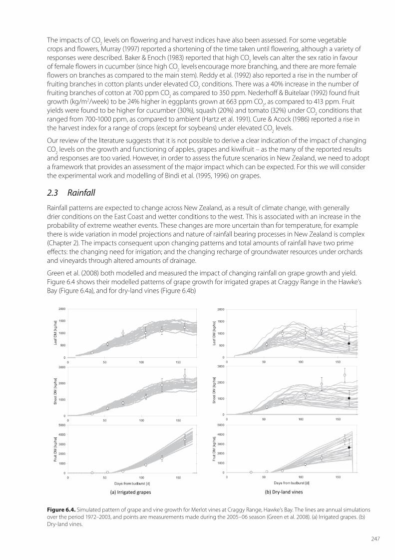
Green et al. (2008) both modelled and measured the impact of changing rainfall on grape growth and yield. Figure 6.4 shows their modelled patterns of grape growth for irrigated grapes at Craggy Range in the Hawke’s Bay (Figure 6.4a), and for dry-land vines (Figure 6.4b)

(a) Irrigated grapes (b) Dry-land vines

Figure 6.4. Simulated pattern of grape and vine growth for Merlot vines at Craggy Range, Hawke’s Bay. The lines are annual simulations over the period 1972–2003, and points are measurements made during the 2005–06 season (Green et al. 2008). (a) Irrigated grapes. (b) Dry-land vines.

248

Figure 6.4a shows that, with irrigation, the year-to-year variation is low, compared to the dry-land vines (Figure 6.4b). The average yield of fruit for the dry-land grapes is also about two-thirds that of the irrigated grapes.

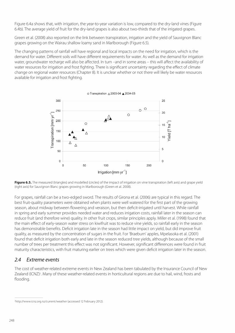
Green et al. (2008) also reported on the link between transpiration, irrigation and the yield of Sauvignon Blanc grapes growing on the Wairau shallow loamy sand in Marlborough (Figure 6.5).

The changing patterns of rainfall will have regional and local impacts on the need for irrigation, which is the demand for water. Different soils will have different requirements for water. As well as the demand for irrigation water, groundwater recharge will also be affected. In turn –and in some areas – this will affect the availability of water resources for irrigation and frost fighting. There is significant uncertainty regarding the effect of climate change on regional water resources (Chapter 8). It is unclear whether or not there will likely be water resources available for irrigation and frost fighting.

Figure 6.5. The measured (triangles) and modelled (circles) of the impact of irrigation on vine transpiration (left axis) and grape yield (right axis) for Sauvignon Blanc grapes growing in Marlborough (Green et al. 2008).

For grapes, rainfall can be a two-edged sword. The results of Girona et al. (2006) are typical in this regard. The best fruit-quality parameters were obtained when plants were well watered for the first part of the growing season, about midway between flowering and veraison, but then deficit-irrigated until harvest. While rainfall in spring and early summer provides needed water and reduces irrigation costs, rainfall later in the season can reduce fruit (and therefore wine) quality. In other fruit crops, similar principles apply. Miller et al. (1998) found that the main effect of early-season water stress on kiwifruit was to reduce vine yields, so rainfall early in the season has demonstrable benefits. Deficit irrigation late in the season had little impact on yield, but did improve fruit quality, as measured by the concentration of sugars in the fruit. For ‘Braeburn’ apples, Mpelasoka et al. (2001) found that deficit irrigation both early and late in the season reduced tree yields, although because of the small number of trees per treatment this effect was not significant. However, significant differences were found in fruit maturity characteristics, with fruit maturing earlier on trees which were given deficit irrigation later in the season.

2.4 Extreme events

The cost of weather-related extreme events in New Zealand has been tabulated by the Insurance Council of New Zealand (ICNZ)2. Many of these weather-related events in horticultural regions are due to hail, wind, frosts and flooding.

2http://www.icnz.org.nz/current/weather (accessed 12 February 2012).

249

The 2009 hail storm in the Bay of Plenty was estimated as costing some NZ$10m3 . However, the ICNZ reported the losses to be NZ$2.3m4. In 1994, the apple industry in the Hawke’s Bay was hit by a hail storm, and the total cost was assessed by the ICNZ to be NZ$14.6 m, most of which would have been due to lost apple production costs and damage to trees.

In Australia, apple growing in Batlow, NSW, is so regularly affected by hail and frost that overhead hail netting is now the norm, as are overhead sprinklers to combat frost. In Shepparton, Victoria, extreme temperatures are now so common that shade cloth and overhead sprinklers are used to cool the fruit during the middle of hot days.

The horticultural industries in Australia, and also in New Zealand, are easily capable of strategic adaptation, as such adaptations are already commonplace To fight frosts and prevent hail damage, there has been a rise in the number of netted orchards in New Zealand, plus widespread use of wind turbines, overhead sprinklers, as well as the use of helicopters. Given the impact that early- or late-season extreme events can have on fruit production and quality, investment in strategic adaptation measures is now seen as being justified.

Table 6.1 presents a summary of the impacts of the various facets of climate change for the main horticultural industries in New Zealand, as has been discussed above.

Table 6.1. Summary of climate-change impacts for the main horticultural industries in New Zealand.

Apples Grapes KiwifruitTemperature

Temperature means Yield

Quality

Disease risk

Sunburn

Yield

Quality

Disease risk

Yield

Quality (and )

Disease risk

Temperature extremes

Frost

Heatwaves

Frost damage Frost damage Frost damage

CO2 Biomass Biomass Biomass

Rainfall variability Irrigation Irrigation

Drought risk

Irrigation

Water quality Leachate load Leachate load Leachate load

Extreme events

Hail ~

Wind ~

Damage to fruit ~

Damage to trees ~

Damage to fruit ~

Damage to vines ~

Damage to fruit ~

Damage to vines ~

Combined impacts ~ unless pest & disease impacts override

unless pest & disease impacts override

~ impact uncertain general increase general decreaase

3http://www.stuff.co.nz/business/industries/2428173/Hail-costs-kiwifruit-growers-10m (accessed 12 February 2012).4http://www.icnz.org.nz/current/weather (accessed 12 February 2012).

250

3 Horticultural adaptation

3.1 Adaptive capacity

To assess possible adaptations in response to climate change, we followed the tri-level scheme of Stokes & Howden (2010) as set out in Chapter 1. These types of adaptation are:

. Tactical adaptation: This involves modifying production practices within the current system, which in horticulture might involve different sprays, irrigation practices, pest management strategies, or pruning practices.

. Strategic adaptation: At this second level, a change is made to the current production system in a substantive way which in horticulture might mean a change in cultivar, a change in the wine-making process, a change to the tree/vine support trellising system, or the installation of netting for hail protection or shade.

. Transformational adaptation: At the highest level, adaptation involves adoption of a new production system, or a change in the location of the industry. In horticulture, this could be the development of new plantings of a new crop in a new region, or new plantings of an existing crop in a different region. This would also result in infrastructural changes.

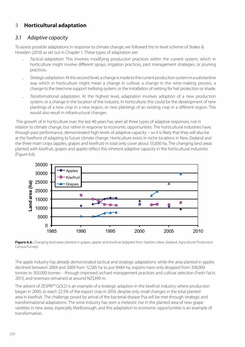
The growth of in horticulture over the last 40 years has seen all three types of adaptive responses, not in relation to climate change, but rather in response to economic opportunities. The horticultural industries have, through past performance, demonstrated high levels of adaptive capacity – so it is likely that they will also be at the forefront of adapting to future climate change. Horticulture exists in niche locations in New Zealand and the three main crops (apples, grapes and kiwifruit) in total only cover about 55,000 ha. The changing land areas planted with kiwifruit, grapes and apples reflect this inherent adaptive capacity in the horticultural industries (Figure 6.6).

0

5000

10000

15000

20000

25000

30000

35000

1985 1990 1995 2000 2005 2010

Land

are

a (h

a)

Apples

Kiwifruit

Grapes

Figure 6.6. Changing land areas planted in grapes, apples and kiwifruit (adapted from Statistics New Zealand, Agricultural Production Census/Survey).

The apple industry has already demonstrated tactical and strategic adaptations: while the area planted in apples declined between 2004 and 2009 from 12,585 ha to just 8484 ha, exports have only dropped from 358,000 tonnes to 303,000 tonnes – through improved orchard management practices and cultivar selection (Fresh Facts 2011), and revenues remained at around NZ$390 m.

The advent of ZESPRI™ GOLD is an example of a strategic adaption in the kiwifruit industry; where production began in 2000, to reach 22.5% of the export crop in 2010, despite only small changes in the total planted area in kiwifruit. The challenge posed by arrival of the bacterial disease Psa will be met through strategic and transformational adaptations. The wine industry has seen a meteoric rise in the planted area of new grape varieties in new areas, especially Marlborough, and this adaptation to economic opportunities is an example of transformation.

251

Given the demonstrated capacity for adaptive management in the horticultural industries, the challenges posed by climate change will lead to future tactical and strategic adaptations in existing horticultural regions, and transformational changes by expansion into new areas. We will detail these in relation to the various impacts posed by climate change.

Putland et al. (2011) found that adaptation measures to the main impacts of climate change could include: . new varieties

. dormancy-breaking compounds

. hail and shade netting

. orchard design

. crop load manipulation

. deficit irrigation strategies

. root-stock selection.

Most of these are tactical, and some are strategic adaptations. An interesting finding in this report, and which was reinforced by the recent work on winter chilling in Australia by Darbyshire et al. (2011), is that the existing variation in climate between fruit growing regions in Australia is much greater than the likely change in climate at any given site between now and 2050. So, the adaptation measures we will see in some of the more favourable future growing regions are already in operation in some of the regions currently less favoured for fruit growth. This space-time interaction is also presently in action in New Zealand, and we can look to a future extension of current adaptation measures in some regions into other areas that presently might not need them as much.

Box 6.1. Impacts and adaptations for the commercial vegetable industry.

Commercial vegetable production makes a large contribution to New Zealand’s economy, both via domestic revenues and through export earnings. Export revenues for the 2010/2011 growing season were NZ$614M, of which NZ$270M was for fresh produce. This included onions (NZ$110M), squash (NZ$64M), capsicums (NZ$36M). There were export earnings of NZ$344M from processed vegetables which included frozen potatoes (NZ$81M), peas (NZ$82M), beans (NZ$44M), and sweetcorn NZ$41M) (Fresh Facts 2011). Australia and Japan are the major destinations for New Zealand’s vegetable exports.

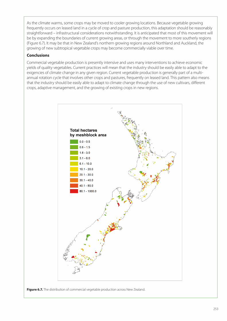
Domestically, earning from potatoes dominated (NZ$451M), but sales of greenhouse tomatoes (NZ$108M), brassicas (NZ$80M), peas (NZ$50M), lettuce (NZ$42M), carrots (NZ$30M), and capsicums (NZ$29M) were also significant. Production is widely spread throughout the country (Figure 6.7), with the major production regions being Canterbury, Hawke’s Bay, Auckland, Manawatu-Wanganui, Gisborne, and Waikato (Fresh Facts 2011).

Vegetable production is intensive, often with multiple crop cycles per year. Fertiliser use, pesticide sprays, irrigation and other interventions mean that productivity is often more a measure of technological inputs, than of the ecosystem services which flow from the local natural-capital stocks of soil, water and climate. Adapting to the impacts of climate change will, in general, result from changed technological interventions. Commercial vegetable production is generally also part of a rotation cycle of different land uses, for both soil health and disease reasons. This frequently involves use of leased land by commercial vegetable growers, so there is a wide range of adaptation measures available, from changing technologies, changing locations, and changing crops.

Impacts of climate change

Temperature

Increased temperatures will extend the potential growing season for many vegetable crops, for example lettuce (Pearson et al. 1997) and tomato (Maltby 1995). By allowing earlier planting and later harvest, there could be more cycles of crop production in a year. The period of growth for a particular cultivar will generally be reduced too, as higher temperatures will enable more rapid plant development. For some crops, especially green-leaf crops such as lettuce, an additional rotation may become possible within the growing season at some locations. However, the shortened period from planting to harvest can impact negatively on vegetable quality. For example, higher temperatures can lead to ‘bolting’ (premature development of the seed head) in some crops (Dioguardi 1995). The timing of the harvest window will become more important. Wurr et al. (1996) found that the optimum

252

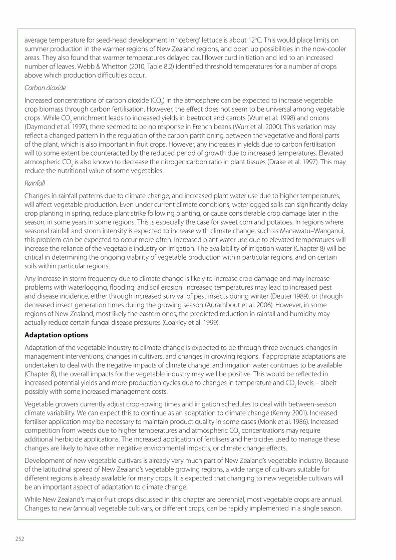
average temperature for seed-head development in ‘Iceberg’ lettuce is about 12oC. This would place limits on summer production in the warmer regions of New Zealand regions, and open up possibilities in the now-cooler areas. They also found that warmer temperatures delayed cauliflower curd initiation and led to an increased number of leaves. Webb & Whetton (2010, Table 8.2) identified threshold temperatures for a number of crops above which production difficulties occur.

Carbon dioxide

Increased concentrations of carbon dioxide (CO2) in the atmosphere can be expected to increase vegetable crop biomass through carbon fertilisation. However, the effect does not seem to be universal among vegetable crops. While CO2 enrichment leads to increased yields in beetroot and carrots (Wurr et al. 1998) and onions (Daymond et al. 1997), there seemed to be no response in French beans (Wurr et al. 2000). This variation may reflect a changed pattern in the regulation of the carbon partitioning between the vegetative and floral parts of the plant, which is also important in fruit crops. However, any increases in yields due to carbon fertilisation will to some extent be counteracted by the reduced period of growth due to increased temperatures. Elevated atmospheric CO2 is also known to decrease the nitrogen:carbon ratio in plant tissues (Drake et al. 1997). This may reduce the nutritional value of some vegetables.

Rainfall

Changes in rainfall patterns due to climate change, and increased plant water use due to higher temperatures, will affect vegetable production. Even under current climate conditions, waterlogged soils can significantly delay crop planting in spring, reduce plant strike following planting, or cause considerable crop damage later in the season, in some years in some regions. This is especially the case for sweet corn and potatoes. In regions where seasonal rainfall and storm intensity is expected to increase with climate change, such as Manawatu–Wanganui, this problem can be expected to occur more often. Increased plant water use due to elevated temperatures will increase the reliance of the vegetable industry on irrigation. The availability of irrigation water (Chapter 8) will be critical in determining the ongoing viability of vegetable production within particular regions, and on certain soils within particular regions.

Any increase in storm frequency due to climate change is likely to increase crop damage and may increase problems with waterlogging, flooding, and soil erosion. Increased temperatures may lead to increased pest and disease incidence, either through increased survival of pest insects during winter (Deuter 1989), or through decreased insect generation times during the growing season (Aurambout et al. 2006). However, in some regions of New Zealand, most likely the eastern ones, the predicted reduction in rainfall and humidity may actually reduce certain fungal disease pressures (Coakley et al. 1999).

Adaptation options

Adaptation of the vegetable industry to climate change is expected to be through three avenues: changes in management interventions, changes in cultivars, and changes in growing regions. If appropriate adaptations are undertaken to deal with the negative impacts of climate change, and irrigation water continues to be available (Chapter 8), the overall impacts for the vegetable industry may well be positive. This would be reflected in increased potential yields and more production cycles due to changes in temperature and CO2 levels – albeit possibly with some increased management costs.

Vegetable growers currently adjust crop-sowing times and irrigation schedules to deal with between-season climate variability. We can expect this to continue as an adaptation to climate change (Kenny 2001). Increased fertiliser application may be necessary to maintain product quality in some cases (Monk et al. 1986). Increased competition from weeds due to higher temperatures and atmospheric CO2 concentrations may require additional herbicide applications. The increased application of fertilisers and herbicides used to manage these changes are likely to have other negative environmental impacts, or climate change effects.

Development of new vegetable cultivars is already very much part of New Zealand’s vegetable industry. Because of the latitudinal spread of New Zealand’s vegetable growing regions, a wide range of cultivars suitable for different regions is already available for many crops. It is expected that changing to new vegetable cultivars will be an important aspect of adaptation to climate change.

While New Zealand’s major fruit crops discussed in this chapter are perennial, most vegetable crops are annual. Changes to new (annual) vegetable cultivars, or different crops, can be rapidly implemented in a single season.

253

As the climate warms, some crops may be moved to cooler growing locations. Because vegetable growing frequently occurs on leased land in a cycle of crop and pasture production, this adaptation should be reasonably straightforward – infrastructural considerations notwithstanding. It is anticipated that most of this movement will be by expanding the boundaries of current growing areas, or through the movement to more southerly regions (Figure 6.7). It may be that in New Zealand’s northern growing regions around Northland and Auckland, the growing of new subtropical vegetable crops may become commercially viable over time.

Conclusions

Commercial vegetable production is presently intensive and uses many interventions to achieve economic yields of quality vegetables. Current practices will mean that the industry should be easily able to adapt to the exigencies of climate change in any given region. Current vegetable production is generally part of a multi-annual rotation cycle that involves other crops and pastures, frequently on leased land. This pattern also means that the industry should be easily able to adapt to climate change through the use of new cultivars, different crops, adaptive management, and the growing of existing crops in new regions.

Figure 6.7. The distribution of commercial vegetable production across New Zealand.

254

3.1.1 Tactical adaptation

Tactical adaptations are considered as means to: control increased summer vegetative growth; control sunburn; maintain flower numbers in kiwifruit; deal with extreme events; maintain irrigation requirements; and use the best cultivars.

Control of summer vegetative growth . Changed winter pruning systems. Presently, all fruit trees and vines are extensively pruned each winter,

with considerable flexibility possible to control the number and types of buds available to provide flowers and vegetative shoots in the following season. By manipulating this balance, growers can alter crop load to an appropriate level for the expected conditions, and also to some extent alter the vegetative/floral balance of the tree, or vine. In the case of vine crops such as grapes and kiwifruit, excessive vegetative vigour in summer can lead to reduced fruit size and/or quality, so control of the vegetative/floral balance following climate change will be very important. One likely tactical adaptation would be the laying down of weaker (thinner) canes in the winter, to reduce summer vegetative growth.

. Changed summer pruning systems. While winter pruning is necessary in all fruit crops, summer pruning is an additional cost which growers try to minimise. In apples, little summer pruning is needed. In grapes, vines are generally pruned mechanically, so if warmer summer temperatures lead to increased vegetative growth that cannot be controlled by winter pruning, additional pruning may be necessary leading to increased costs. In kiwifruit, many different approaches are taken to summer pruning to control vegetative growth, including ‘zero leafing’ where shoots are pruned immediately after the last fruit on the shoot, suppressing any vegetative regrowth on that shoot. As summer temperatures increase, it can be expected that the use of such techniques will increase.

. Girdling. In kiwifruit, cane and trunk girdling have been used in recent years by many growers to increase dry matter partitioning to the fruit (in preference to storage organs such as roots or trunk). This technique does have some potential downsides: with the outbreak of the Psa disease, the use of girdling in the industry has been reduced in response to fears of providing additional infection sites. It is likely that this technique will continue to be used to offset the effects of increased vegetative competition. In the future, girdling may prove to be an appropriate management technique for fruit crops other than just kiwifruit.

Control of sunburn in apples . In hot summers, apples exposed to full sunlight can overheat and suffer ‘sunburn’ (Wünsche et al. 2004).

The incidence of this disorder can be expected to increase with climate change. A partial adaptation to a potential increase in apple sunburn is to use winter pruning (discussed above) to increase partitioning to vegetative growth, increasing the number of leaves and shading. Fruit or flower thinning could also be used to remove exposed fruit. A more effective approach currently being used by some growers is the installation of multi-purpose overhead netting which provides shade, thereby giving protection from sunburn, and also (discussed below) protection from hail and even extreme wind events.

Maintenance of flower numbers in kiwifruit . In grapes and apples, it is likely that adequate flower numbers will be maintained as temperatures increase,

as both these crops receive more than adequate chilling in their current growing environments and this is not seen as a limitation. In apples considerable chemical (or manual) flower thinning is currently carried out. In kiwifruit, however, hydrogen cyanamide (HC) is currently used to induce flowering. However, its future use is in doubt because of health concerns resulting from spraying. An alternative is being sought. Failure to realise this might require strategic or transformation adaptation measures.

Increased frequencies of extreme events . With global warming, spring and autumn frosts in certain parts of the country are likely to become less

common. Storms with associated hail and strong winds may well also become more frequent, although this is less certain than the changes in frost frequency (Chapter 2). A single hail storm at the wrong time of year can damage an entire fruit crop, rendering it unsuitable for sale. Strong winds can break growing shoots, particularly in spring, and can also cause considerable fruit drop and damage if they occur late in the growing season. Some protection from increased wind could be provided by more shelter belts of

255

trees, or vertical netting between orchard blocks. To protect against hail the only real option is overhead netting, which is already in common use on some orchards. However, all these options are expensive. The capital cost of netting, particularly overhead netting, is very high; and shelter trees are seen as ‘expensive’ because they remove land from fruit production. Tactical adaptation to these extreme events is likely to be very dependent on economic factors, such as profitability of the crop.

Increased irrigation requirements . With the prospect of drier conditions in New Zealand’s major horticultural regions, the use of irrigation

is likely to become more widespread. Presently, irrigation is used in the major grape and apple growing regions. However, in Hawke’s Bay and Marlborough, the irrigation resource is already fully allocated, and so better use of irrigation water will be required. This will be possible through better scheduling of the optimum amount of water and applying it only at the time required to achieve the desired outcome. For kiwifruit in the Bay of Plenty for example only some 10% to 20% of the crop appears to be irrigated. This might increase as conditions become drier. The impact of climate change on water resources is unclear (Chapter 8), so the question of whether the required irrigation water will be available in sufficient quantity cannot yet be answered with any certainty

Changing cultivars . For grapes in particular, with warmer conditions, new cultivars might replace those currently being grown.

As shown in Figure 6.3, the Huglin Index provides an indication of which cultivars would suit warmer conditions. Meanwhile for all of the fruit crops, active breeding programmes are underway to develop not only new fruit with desired consumer traits, but also those that will be better adapted to future conditions, such as ones that might have longer seasonal growth requirements. This adaptation could be either tactical (top grafting new budwood), or strategic (new plantings), and is discussed below in more detail.

3.1.2 Strategic adaptation

New variety development is likely to be a major factor in strategic adaptation to climate change. Different cultivars of fruit crops are known to grow better in some regions than others, leading to some regions becoming well known for particular varieties, for example ‘Marlborough Sauvignon Blanc’. As regional climates change, it is likely that some cultivars will become more suitable for growing and others less so. In apples and grapes a large range of commercial varieties are already available for growers to choose from. As indications appear that certain cultivars are performing less well in a region, the industry will have a range of alternatives which can be tested. While cultivar change in the (perennial) fruit industry takes longer than it does for annual crops, such change happens regularly now for reasons associated with customer demand and profitability. This is at a pace sufficiently rapid to cope with the demands of climate change as long as appropriate cultivars are available. In the kiwifruit industry, the number of commercial cultivars available currently is somewhat smaller than in apples or grapes, but ZESPRI™ have identified regular release of new cultivars as an essential part of their long-term planning. An active breeding programme carried out by Plant & Food Research is providing a stream of potential new cultivars with desirable characteristics; and the ability to produce adequate flower numbers in warmer winters has been identified as a factor to consider. An overview of this programme can be found on the Plant & Food website5.

New irrigation schemes are being mooted around New Zealand, and financial support for these is coming through the Government’s Irrigation Acceleration Fund. These schemes will enable strategic adaptation to the drier conditions that are likely in eastern and northern regions in the future. Detention storage is being proposed for irrigation water, inter alia, in the Ruataniwha basin in central Hawke’s Bay, on the Ruamahanga River in the Wairarapa, and in the Hurunui basin of Canterbury. This water will not only be available for summer irrigation, but also for frost fighting as these areas are cooler than where horticultural crops are currently grown.

3.1.3 Transformational adaptation

Transformational adaptation to climate change could see horticulture move into new regions where production is currently limited due to cooler and sub-optimal conditions. As shown in Figure 6.6, the horticultural industries

5http://www.plantandfood.co.nz/page/our-research/breeding-genomics/capabilities/breeding (accessed 8 April 2012).

256

are well capable of transformational change in response to economic opportunities, and this could well happen in response to climate change. The rapid and complete transformation of Marlborough over 25 years from a pastoral economy to one largely based on grapes is a good example of how such change can occur. Similarly, the transformation of the ‘poor’ soils north of Flaxmere in the Hawke’s Bay to the wine-growing appellation of the Gimblett Gravels is another example of how massive change can occur rapidly in response to external drivers.

For horticulture, there are many areas into which the industry could move if the growing conditions in extant regions become compromised because of climate change. These could include: the Mamaku Plateau between Rotorua and Hamilton; the Ruataniwha basin of central Hawke’s Bay; the Wairarapa; the downlands between Wanganui and Waverly; the Whangaehu Valley near Whanganui; the Hurunui Basin in Canterbury; the river flats of the Waitaki River; the Hakataramea Basin; the Maniototo Valley near Ranfurly; and the upper Clutha Valley. There are already small pockets of horticulture in these regions, and so some local knowledge of current conditions already exists. Infrastructure would be a limitation to expansion that would require land and infrastructural investment in order to enable the transformation of new regions into horticulture.

3.2 Adaptation summary

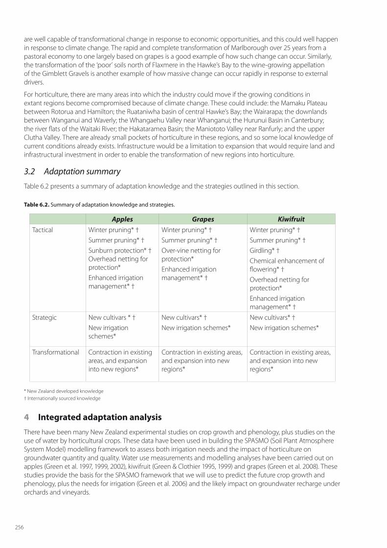
Table 6.2 presents a summary of adaptation knowledge and the strategies outlined in this section.

Table 6.2. Summary of adaptation knowledge and strategies.

Apples Grapes KiwifruitTactical Winter pruning* †

Summer pruning* †Sunburn protection* † Overhead netting for protection*Enhanced irrigation management* †

Winter pruning* †Summer pruning* †Over-vine netting for protection*Enhanced irrigation management* †

Winter pruning* †Summer pruning* †Girdling* †Chemical enhancement of flowering* †Overhead netting for protection*Enhanced irrigation management* †

Strategic New cultivars * †New irrigation schemes*

New cultivars* †New irrigation schemes*

New cultivars* †New irrigation schemes*

Transformational Contraction in existing areas, and expansion into new regions*

Contraction in existing areas, and expansion into new regions*

Contraction in existing areas, and expansion into new regions*

* New Zealand developed knowledge† Internationally sourced knowledge

4 Integrated adaptation analysis

There have been many New Zealand experimental studies on crop growth and phenology, plus studies on the use of water by horticultural crops. These data have been used in building the SPASMO (Soil Plant Atmosphere System Model) modelling framework to assess both irrigation needs and the impact of horticulture on groundwater quantity and quality. Water use measurements and modelling analyses have been carried out on apples (Green et al. 1997, 1999, 2002), kiwifruit (Green & Clothier 1995, 1999) and grapes (Green et al. 2008). These studies provide the basis for the SPASMO framework that we will use to predict the future crop growth and phenology, plus the needs for irrigation (Green et al. 2006) and the likely impact on groundwater recharge under orchards and vineyards.

257

4.1 The SPASMO modelling framework

Since SPASMO is a fully mechanistic model that accounts for all flows of water into and out of the root-zone soil of orchards and vineyards, it is possible to assess the drainage of water leaving the root-zone destined for recharge of the underlying groundwater (see Appendix A). As SPASMO takes into account the carbon and nitrogen cycles, it is possible to predict the impact on the underlying groundwater of nutrient leaching (Clothier et al. 2008). In a recent study on the water footprint of kiwifruit, Deurer et al. (2011) used SPASMO to assess the blue-water footprint of groundwater recharge, along with the grey-water footprint due to leaching losses of nitrate. This modelling approach is also used here to predict the changing quantity and quality of groundwater recharge under climate change for apples, grapes and kiwifruit.

Our modelling was carried out using our SPASMO modelling tool. SPASMO is a mechanistic biophysical model that operates on a daily time-step (Green et al. 2008). Current orchard practices will be assumed to assess impacts in the future centred on 2050. Unlike the analyses in the other chapters, our 2050 scenarios will derive from assessing impacts over the time period 2030–2070, so that we can assess temporal variability and consider extreme events over longer time periods for these three perennial tree or vine crops. Two future scenarios will be considered, based on the IPCC AIB/A2 ‘high’ scenario, and the ‘low’ B1 scenario. As described in Chapter 2, these scenarios have been scaled down to the local level in New Zealand using finer resolution Regional Climate Models. These will be compared with current conditions, being derived from our modelling of the period 1972–2010. We will assess the impacts in relation to the three climate drivers of a CO2 increase, the changing temperature, and changing patterns of rainfall.

4.1.1 Biomass response

Bindi et al. (1995) developed a model for simulating the growth and yield of a grapevine. The main processes they simulated were: crop ontogeny, leaf development, biomass accumulation and fruit growth. Bindi et al. (1995) found an enhancement of vine growth under elevated CO2 conditions. They expressed this enhancement in relation to an overall increase in the ratio of intercepted radiation to biomass accumulation, which they termed the Radiation Utilisation Efficiency (RUE).They found that the RUE increased linearly at 0.1% ppm-1 (i.e. 0.001 ppm-1) with increasing CO2 concentration [CO2], and that:

RUE[CO2] – RUE[353] {1 + a ([CO2] – 353)}

where a is the constant 0.001 ppm-1, and RUE[353] is the RUE at CO2 concentration of 353 ppm. Importantly for our modelling exercise, they found that none of the other modelling parameters were considered to be affected by changing the CO2 concentration.

This relationship will be used, not only for grapes, but also for apples and kiwifruit, for we have no other information on the CO2 response of those specific crops. This rate of increase of the RUE with CO2 concentration lies within the range suggested for the increase in light-saturated leaf photosynthesis with the CO2 concentration across the range of crops in the meta-analysis of Ainsworth & Rogers (2007). The modelling here considers that the increase biomass accumulation will respond to the rise in CO2, whilst maintaining the same allometric rules of allocation to other plant parts. This will provide a first order assessment of the impact of CO2 on tree and vine growth, and potential crop yields.

4.1.2 Development response

In the present desktop study, our results for grapes are limited to modelling the impact on the timing of flower development. However, there is information available on the impact of winter chilling on flower numbers for kiwifruit (Hall et al. 2001; Snelgar et al. 2008). Snelgar et al. (2008) found number of king flowers per winter bud, that is FlowersWB, to be given by:

FlowersWB = 3.8–0.24(T567) + 0.04(HC)(T567) r2 = 0.77

where (T567) is the mean temperature for May, June, July, and (HC) = 1 if hydrogen cynamide (HC) is applied, 0 if not. Note however this model appears to underestimate the temperature effect at a given site. An alternative model is found where:

258

FlowersWB = -0.5 + 0.40(TAnnual) – 0.45(T567) + 0.05(HC)(T567) r2 = 0.87

Here TAnnual is the mean annual temperature. This model fitted the commercial kiwifruit data better. This approach is used to model flower numbers and their impact on kiwifruit yield. Also, soil water deficits are taken into account in modelling fruit yield (Green et al. 2009).

4.1.3 Quality and yield response

For grapes, Parker et al. (2011) developed a phenological model to predict bud break, flowering and veraison. The time of flowering and of veraison were both calculated by accumulating growing degree days, based on daily (Tmax+Tmin)/2 temperatures, with a base 0°C, starting from day of year (DOY) 60 (i.e., 01 March) of the year for the Northern Hemisphere. They found flowering occurs when the following total degree-days were achieved: 1238 for Sauvignon Blanc and 1219 for Pinot Noir. Veraison occurs at 2517 for Sauvignon Blanc and 2507 for Pinot Noir. This model was calibrated for Marlborough conditions by taking day 1 to be 01 September, and so for Sauvignon Blanc the mean and standard deviation were found to be:

. Bud break 409 ± 68 GDD (n = 30)

. Flowering 1357 ± 68 GDD (n = 30)

. Veraison 2496 ± 173 GDD (n = 25)

Here GDD is growing degree days with based 0°C. Chuine et al. (2004) suggested that the time-to-harvest is a fixed number of days after veraison. It is 33.5 days for Pinot Noir. Our analysis for Marlborough Sauvignon Blanc suggests that harvest date is on average 43 (± 7) days after veraison, although it depends on crop load, with four-cane vines being harvested some nine days later. For the purpose of modelling harvest date we have derived parameters for Brix development, and assumed harvest date occurs when Brix = 21.5°.

Trought (2005) presented a simple model for the berry yield of Sauvignon Blanc in Marlborough based on temperature, namely:

Yield (t/ha) = A*Tinitiation + B*Tflowering + C

where Tinitiation is the average daily GDD base 10°C from 11 Dec to 17 Jan in the previous season, and Tflowering = average daily GDD base of 10°C from 9 Dec to 9 Jan of the current season. Trought (2005) found A = 2.73, B = 2.92, and C = -29.48.

For apples, Austin &Hall (2001) developed temperature-driven models for the date of bloom and date of harvest using the data presented by Stanley et al. (2000). For the date of full bloom of typical mid-season apples, such as Gala, they found:

Date (1 Jan = day 1) of Full bloom = 367 – 5.5 Tx,Aug-Sep

Where, Tx,Aug-Sep = average maximum temperature from 1 August to 30 September; and for the date of harvest they found:

Days from Full bloom to Maturity = 263.2 – 7.62 T0-50 DAFB

where T0-50 DAFB = true mean temperature for the first 50 days after full bloom. These results from the baseline reference for current conditions, and then SPASMO is used to predict the future changes in bloom and maturity dates.

For kiwifruit there have been developed temperature-driven models of bud break (Hall & McPherson, 1997a), flowering (McPherson et al. 1992) and harvest maturity (Hall & McPherson, 1997b). The model of bud break (Hall & McPherson, 1997a) considers a state variable S, set to zero on day D0, and which is incremented each day according to the weather. Bud break occurs on the day when S>=1. Each day, the state variable is incremented by:

259

)()()())(1( ThSwTcSwdS +=

where c(T) and h(T) are ‘chilling’ and ‘warming’ responses respectively, and w(S) is a weighting function which changes from 0 to 1 as S progresses from 0 to 1. The flowering date model of McPherson et al. (1992) also considers a state variable S and which is set to zero at bud break and then accumulates daily increments according to:

TdS 00228.00161.0 +=

where T is the mean temperature for the day. Flowering occurs when S reaches 1. For predicting the time to reach maturity for harvest, Hall & McPherson (1997b) found that the late-season temperatures had a major effect on the time to reach commercial maturity (6.2 °Brix) in kiwifruit. The soluble solids level (SS) was assumed to start at 4.5 o Brix, some a0 days after flowering, and then then accumulate by:

dteaaKdSS Tp= )( 0

after time dt at temperature T, where a is the ‘age’ of the fruit (time since flowering). Parameter values fitted were a0=90 days, K=0.00126, λ=0.185, and p=1.424. Fruit can be harvested once SS reaches 6.2 ° Brix. These temperature-driven models of kiwifruit phenology are used to establish baseline references for SPASMO to predict changes in the seasonality of kiwifruit in the future as well as potential crop yields.

Apple size and weight are metrics of fruit quality. Austin et al. (1999) presented temperature-driven models for both fruit diameter and fruit weight, based on the growth in the mass of both the meristematic and non-meristematic compartments. SPASMO modelling considers these relationships, and enables assessment of how they are likely to change in the future for New Zealand’s apple growing regions.

Fruit size and the dry matter content of the fruit at harvest are key fruit quality criteria for kiwifruit. Snelgar et al. (2007) and Hall & Snelgar (2008) have developed temperature-driven models for predicting the dry matter content of kiwifruit at harvest. They used fruit data collected near Te Puke, and their model, which includes the effect of autumnal temperatures, is:

DM% = (11.3±1.0) + (0.67±0.04)Tspring – (0.66±0.06)Tsummer + (0.54±0.09)Tautumn

where Tspring was a weighted average of October, November, and December temperatures, with relative weightings of ½, 1, and ½ respectively, Tsummer was a simple average of January and February, and Tautumn was a weighted average of April and May, with relative weightings of ½ and 1 respectively. Green (2007) obtained a slightly different regression by including the effect of the average soil water deficit in summer (∆SSummer), and using the simple average of April and May for autumnal temperatures, so:

DM% = 16.42 + 0.4184 Tspring – 0.5506 Tsummer + 0.241 Tautumn + 0.00967∆SSummer

Although there is not currently a peer-reviewed model to predict the absolute value of kiwifruit size from environmental data, there have been models developed which describe the shape of the fruit-growth curve, which is essentially a double sigmoid (Hall et al. 2002; Bebbington et al. 2009). These models can be used to predict final size, once they have been referenced to an early season measurement of fruit size. Green (2006) modelled the fruit fresh weight (FW) for ZESPRITM GREEN at Te Puke using the following equation:

FW = 26.4 + 0.055 GDD - 0.075 ∆SSummer - 0.021 RApril

where GDD is the number of growing degree days (10°C base temperature) for the growing season, and RApril is the late season rainfall in April. This model accounted for 84% of the season-to-season variation in mean fruit FW at Te Puke, and had a standard error of 2.8 g. Warmer temperatures in general will lead to larger fruit. There is a strong negative correlation between fruit FW and soil water deficit (∆S). Fruit FW will be reduced by 7.5 g for every 100 mm of soil water deficit, all other factors being equal. There is a small but negative impact of late season rainfall. These relationships have subsequently been used to deduce the potential of irrigation to alter

260

fruit yield. SPASMO modelling of the dry matter content and fruit fresh weight of future kiwifruit will simply use the equations above. However, if the rise in CO2 results in a rise fruit biomass, as our allometric rule based on RUE predicts, then it would be likely that the growers’ response (i.e., tactical adaptation) would be to adjust crop load to achieve the desired fruit sizes for consumer appeal. Under a future climate there is uncertainty about how the leaf to fruit ratio might change and it is possible that crop load can increase above current levels because there will be greater leaf areas to support the developing fruit.

4.2 Horticulture system indicators

Biomass and productivity. Plant biomass is a useful system indicator for horticultural crops as it offers an insight into the ‘potential’ that could perhaps be achieved with cultivars able to handle future climatic conditions. This also provides a baseline from which to partition sufficient photosynthates and dry matter to the fruit parts of the plant which are the harvested portions of horticultural crops. Yield is a useful indicator for all crops, as a greater volume of fruit can be expected to lead to greater returns, provided of course fruit quality can be maintained. The goal is to produce high-quality fruit, and so the growers seek to ensure the highest possible pack-out from the harvested fruit.

Fruit quality. For fresh apples and kiwifruit there are a range of quality metrics determining the orchard gate returns. Likewise with wine, there are desired berry qualities, and these enable the winemakers to produce wine styles for which consumers will pay a premium.

For kiwifruit there is a well-defined metric in the industry, namely the dry matter percentage of the fruit (%DM). Growers are paid a premium for high DM fruit, so there is developing a good understanding of how to manage this. Other quality metrics include early harvest dates and fruit size.

Important factors for apple quality are texture, flavour, and fruit size. In New Zealand, however, some attention is now being paid to %DM as a quality aspect (Palmer et al. 2010), but models of how this changes with climate have not yet been developed. For fruit size here, the models of Austin et al. (1999) and Austin and Hall (2001) have been applied. This predicts only a small change of less than 5% in apple diameter due to climate change by 2050. SPASMO modelling here suggests that the increase in mean fruit size due to climate change could be even smaller, suggesting that this aspect of apple fruit quality will not be significantly changed by 2050.

Apples

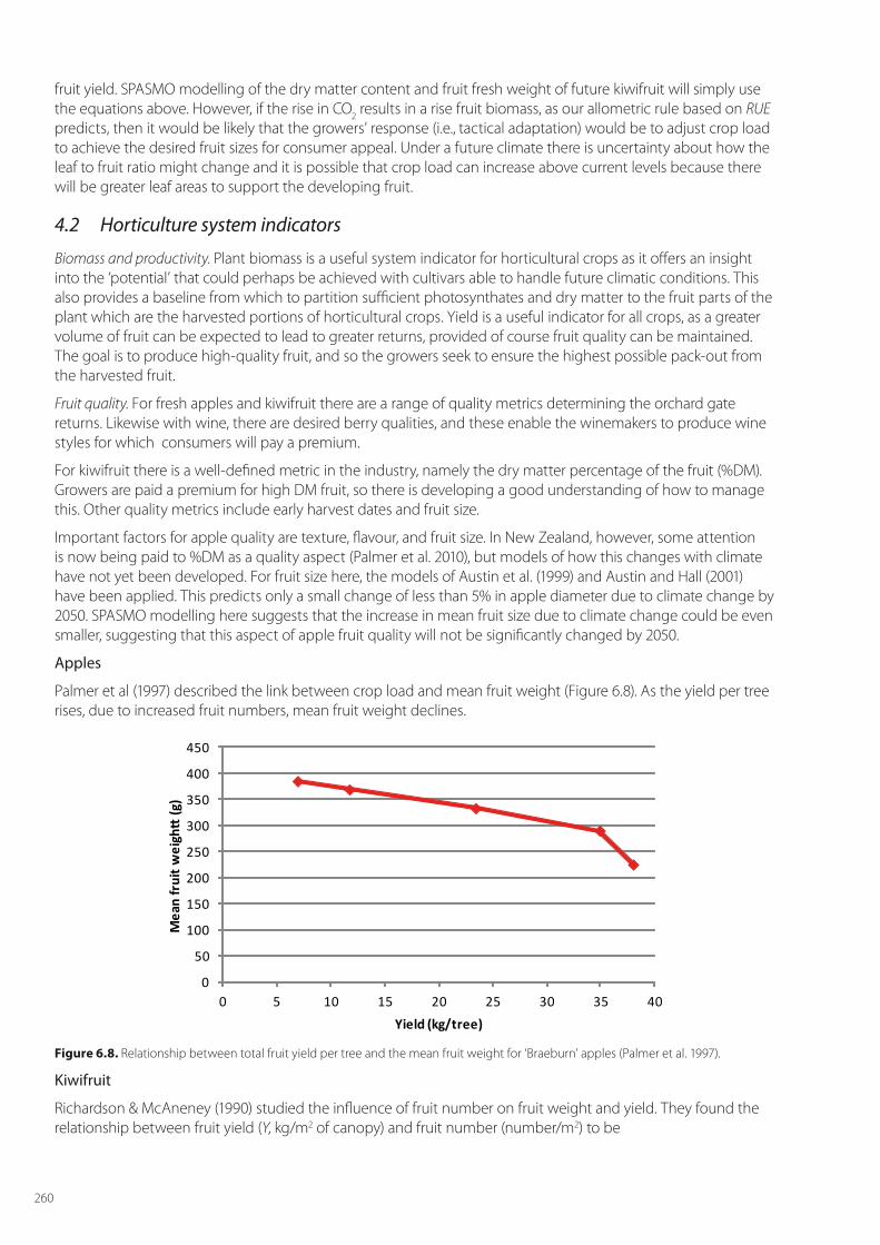
Palmer et al (1997) described the link between crop load and mean fruit weight (Figure 6.8). As the yield per tree rises, due to increased fruit numbers, mean fruit weight declines.

0

50

100

150

200

250

300

350

400

450

0 5 10 15 20 25 30 35 40

Mea

n fr

uit w

eigh

tt (g

)

Yield (kg/tree)

Figure 6.8. Relationship between total fruit yield per tree and the mean fruit weight for ‘Braeburn’ apples (Palmer et al. 1997).

Kiwifruit

Richardson & McAneney (1990) studied the influence of fruit number on fruit weight and yield. They found the relationship between fruit yield (Y, kg/m2 of canopy) and fruit number (number/m2) to be

261

Y = Ymax*(N/(N+K))

where K = 95.25 fruit/m2 and Ymax = 13.48 kg/m2. Since the mean fruit size is μ = Y/N, and N = Y/μ then

Y = Ymax*(Y/ μ)/(Y/(μ+K))

This can be rearranged to give a linear relationship between mean fruit size and yield

μ = (Ymax-Y)/K = 141.5-10.5*Y (mean FW in g)

Grapes

Wine-grape quality is hard to assess, because it can vary according to the style of wine desired. Usually, a particular variety will be harvested at approximately the same Brix level. In the case of Sauvignon Blanc this would be typically around 21.5° Brix, so quality will only be impacted if this level is reached too late in the season, which brings with it increased risks of botrytis and frost damage. The SPASMO modelling presented in Table 6.6 shows that the harvest dates are expected to be considerably earlier following climate change, and so lessening the likely risk of botrytis infection. Regions such as Marlborough where Sauvignon Blanc is currently grown with small risk will remain suitable. Further some other regions, such as Wanganui and Central Otago, may become more suitable for this variety.

Summary

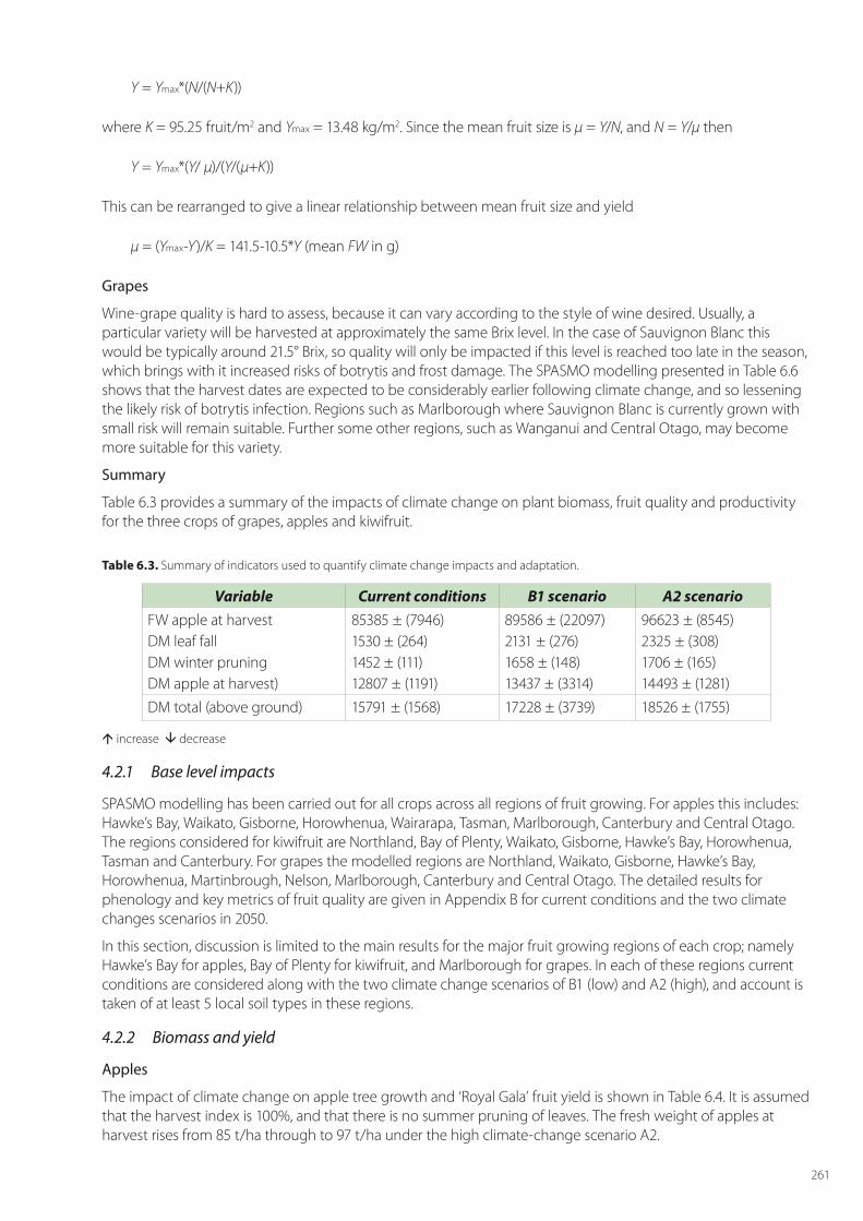
Table 6.3 provides a summary of the impacts of climate change on plant biomass, fruit quality and productivity for the three crops of grapes, apples and kiwifruit.

Table 6.3. Summary of indicators used to quantify climate change impacts and adaptation.

Variable Current conditions B1 scenario A2 scenarioFW apple at harvest DM leaf fall DM winter pruning DM apple at harvest)

85385 ± (7946)1530 ± (264)1452 ± (111)12807 ± (1191)

89586 ± (22097)2131 ± (276)1658 ± (148)13437 ± (3314)

96623 ± (8545)2325 ± (308)1706 ± (165)14493 ± (1281)

DM total (above ground) 15791 ± (1568) 17228 ± (3739) 18526 ± (1755)

increase decrease

4.2.1 Base level impacts

SPASMO modelling has been carried out for all crops across all regions of fruit growing. For apples this includes: Hawke’s Bay, Waikato, Gisborne, Horowhenua, Wairarapa, Tasman, Marlborough, Canterbury and Central Otago. The regions considered for kiwifruit are Northland, Bay of Plenty, Waikato, Gisborne, Hawke’s Bay, Horowhenua, Tasman and Canterbury. For grapes the modelled regions are Northland, Waikato, Gisborne, Hawke’s Bay, Horowhenua, Martinbrough, Nelson, Marlborough, Canterbury and Central Otago. The detailed results for phenology and key metrics of fruit quality are given in Appendix B for current conditions and the two climate changes scenarios in 2050.

In this section, discussion is limited to the main results for the major fruit growing regions of each crop; namely Hawke’s Bay for apples, Bay of Plenty for kiwifruit, and Marlborough for grapes. In each of these regions current conditions are considered along with the two climate change scenarios of B1 (low) and A2 (high), and account is taken of at least 5 local soil types in these regions.

4.2.2 Biomass and yield

Apples

The impact of climate change on apple tree growth and ‘Royal Gala’ fruit yield is shown in Table 6.4. It is assumed that the harvest index is 100%, and that there is no summer pruning of leaves. The fresh weight of apples at harvest rises from 85 t/ha through to 97 t/ha under the high climate-change scenario A2.

262

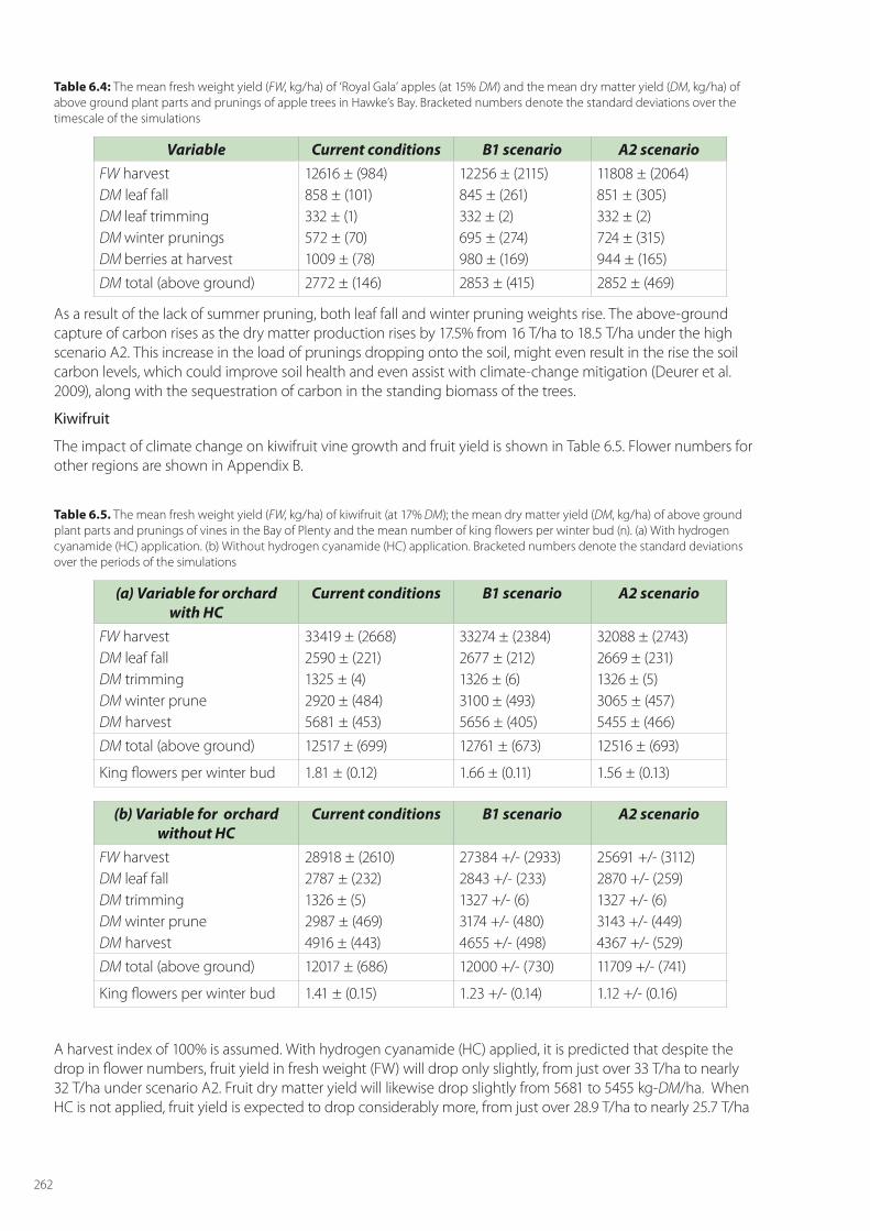
Table 6.4: The mean fresh weight yield (FW, kg/ha) of ‘Royal Gala’ apples (at 15% DM) and the mean dry matter yield (DM, kg/ha) of above ground plant parts and prunings of apple trees in Hawke’s Bay. Bracketed numbers denote the standard deviations over the timescale of the simulations

Variable Current conditions B1 scenario A2 scenarioFW harvestDM leaf fallDM leaf trimmingDM winter pruningsDM berries at harvest

12616 ± (984)858 ± (101)332 ± (1)572 ± (70)1009 ± (78)

12256 ± (2115)845 ± (261)332 ± (2)695 ± (274)980 ± (169)

11808 ± (2064)851 ± (305)332 ± (2)724 ± (315)944 ± (165)

DM total (above ground) 2772 ± (146) 2853 ± (415) 2852 ± (469)

As a result of the lack of summer pruning, both leaf fall and winter pruning weights rise. The above-ground capture of carbon rises as the dry matter production rises by 17.5% from 16 T/ha to 18.5 T/ha under the high scenario A2. This increase in the load of prunings dropping onto the soil, might even result in the rise the soil carbon levels, which could improve soil health and even assist with climate-change mitigation (Deurer et al. 2009), along with the sequestration of carbon in the standing biomass of the trees.

Kiwifruit

The impact of climate change on kiwifruit vine growth and fruit yield is shown in Table 6.5. Flower numbers for other regions are shown in Appendix B.

Table 6.5. The mean fresh weight yield (FW, kg/ha) of kiwifruit (at 17% DM); the mean dry matter yield (DM, kg/ha) of above ground plant parts and prunings of vines in the Bay of Plenty and the mean number of king flowers per winter bud (n). (a) With hydrogen cyanamide (HC) application. (b) Without hydrogen cyanamide (HC) application. Bracketed numbers denote the standard deviations over the periods of the simulations

(a) Variable for orchard with HC

Current conditions B1 scenario A2 scenario

FW harvestDM leaf fallDM trimmingDM winter pruneDM harvest

33419 ± (2668)2590 ± (221)1325 ± (4)2920 ± (484)5681 ± (453)

33274 ± (2384)2677 ± (212)1326 ± (6)3100 ± (493)5656 ± (405)

32088 ± (2743)2669 ± (231)1326 ± (5)3065 ± (457)5455 ± (466)

DM total (above ground) 12517 ± (699) 12761 ± (673) 12516 ± (693)

King flowers per winter bud 1.81 ± (0.12) 1.66 ± (0.11) 1.56 ± (0.13)

(b) Variable for orchard without HC

Current conditions B1 scenario A2 scenario

FW harvestDM leaf fallDM trimmingDM winter pruneDM harvest

28918 ± (2610)2787 ± (232)1326 ± (5)2987 ± (469)4916 ± (443)

27384 +/- (2933)2843 +/- (233)1327 +/- (6)3174 +/- (480)4655 +/- (498)

25691 +/- (3112)2870 +/- (259)1327 +/- (6)3143 +/- (449)4367 +/- (529)

DM total (above ground) 12017 ± (686) 12000 +/- (730) 11709 +/- (741)

King flowers per winter bud 1.41 ± (0.15) 1.23 +/- (0.14) 1.12 +/- (0.16)

A harvest index of 100% is assumed. With hydrogen cyanamide (HC) applied, it is predicted that despite the drop in flower numbers, fruit yield in fresh weight (FW) will drop only slightly, from just over 33 T/ha to nearly 32 T/ha under scenario A2. Fruit dry matter yield will likewise drop slightly from 5681 to 5455 kg-DM/ha. When HC is not applied, fruit yield is expected to drop considerably more, from just over 28.9 T/ha to nearly 25.7 T/ha

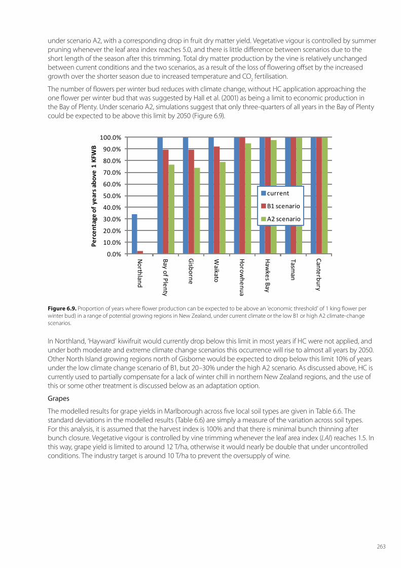
263

under scenario A2, with a corresponding drop in fruit dry matter yield. Vegetative vigour is controlled by summer pruning whenever the leaf area index reaches 5.0, and there is little difference between scenarios due to the short length of the season after this trimming. Total dry matter production by the vine is relatively unchanged between current conditions and the two scenarios, as a result of the loss of flowering offset by the increased growth over the shorter season due to increased temperature and CO2 fertilisation.

The number of flowers per winter bud reduces with climate change, without HC application approaching the one flower per winter bud that was suggested by Hall et al. (2001) as being a limit to economic production in the Bay of Plenty. Under scenario A2, simulations suggest that only three-quarters of all years in the Bay of Plenty could be expected to be above this limit by 2050 (Figure 6.9).

0.0%

10.0%

20.0%

30.0%

40.0%

50.0%

60.0%

70.0%

80.0%

90.0%

100.0%

Northland

Bay of Plenty

Gisborne

Waikato

Horowhenua

Hawkes Bay

Tasman

Canterbury

Perc

enta

ge o

f yea

rs a

bove

1 K

FWB

current

B1 scenario

A2 scenario

Figure 6.9. Proportion of years where flower production can be expected to be above an ‘economic threshold’ of 1 king flower per winter bud) in a range of potential growing regions in New Zealand, under current climate or the low B1 or high A2 climate-change scenarios.

In Northland, ‘Hayward’ kiwifruit would currently drop below this limit in most years if HC were not applied, and under both moderate and extreme climate change scenarios this occurrence will rise to almost all years by 2050. Other North Island growing regions north of Gisborne would be expected to drop below this limit 10% of years under the low climate change scenario of B1, but 20–30% under the high A2 scenario. As discussed above, HC is currently used to partially compensate for a lack of winter chill in northern New Zealand regions, and the use of this or some other treatment is discussed below as an adaptation option.

Grapes

The modelled results for grape yields in Marlborough across five local soil types are given in Table 6.6. The standard deviations in the modelled results (Table 6.6) are simply a measure of the variation across soil types. For this analysis, it is assumed that the harvest index is 100% and that there is minimal bunch thinning after bunch closure. Vegetative vigour is controlled by vine trimming whenever the leaf area index (LAI) reaches 1.5. In this way, grape yield is limited to around 12 T/ha, otherwise it would nearly be double that under uncontrolled conditions. The industry target is around 10 T/ha to prevent the oversupply of wine.

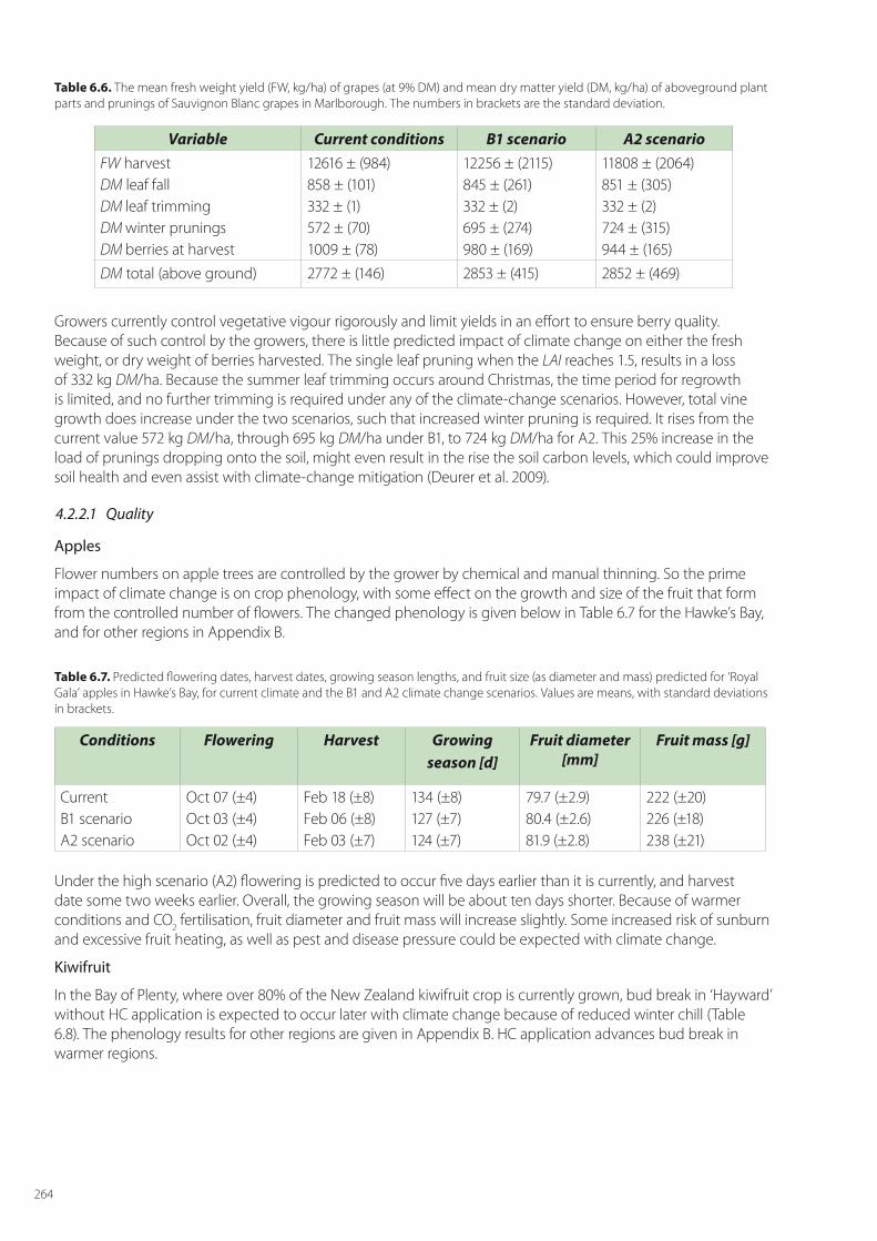
264

Table 6.6. The mean fresh weight yield (FW, kg/ha) of grapes (at 9% DM) and mean dry matter yield (DM, kg/ha) of aboveground plant parts and prunings of Sauvignon Blanc grapes in Marlborough. The numbers in brackets are the standard deviation.

Variable Current conditions B1 scenario A2 scenarioFW harvestDM leaf fallDM leaf trimmingDM winter pruningsDM berries at harvest

12616 ± (984)858 ± (101)332 ± (1)572 ± (70)1009 ± (78)

12256 ± (2115)845 ± (261)332 ± (2)695 ± (274)980 ± (169)

11808 ± (2064)851 ± (305)332 ± (2)724 ± (315)944 ± (165)

DM total (above ground) 2772 ± (146) 2853 ± (415) 2852 ± (469)

Growers currently control vegetative vigour rigorously and limit yields in an effort to ensure berry quality. Because of such control by the growers, there is little predicted impact of climate change on either the fresh weight, or dry weight of berries harvested. The single leaf pruning when the LAI reaches 1.5, results in a loss of 332 kg DM/ha. Because the summer leaf trimming occurs around Christmas, the time period for regrowth is limited, and no further trimming is required under any of the climate-change scenarios. However, total vine growth does increase under the two scenarios, such that increased winter pruning is required. It rises from the current value 572 kg DM/ha, through 695 kg DM/ha under B1, to 724 kg DM/ha for A2. This 25% increase in the load of prunings dropping onto the soil, might even result in the rise the soil carbon levels, which could improve soil health and even assist with climate-change mitigation (Deurer et al. 2009).

4.2.2.1 Quality

Apples

Flower numbers on apple trees are controlled by the grower by chemical and manual thinning. So the prime impact of climate change is on crop phenology, with some effect on the growth and size of the fruit that form from the controlled number of flowers. The changed phenology is given below in Table 6.7 for the Hawke’s Bay, and for other regions in Appendix B.

Table 6.7. Predicted flowering dates, harvest dates, growing season lengths, and fruit size (as diameter and mass) predicted for ‘Royal Gala’ apples in Hawke’s Bay, for current climate and the B1 and A2 climate change scenarios. Values are means, with standard deviations in brackets.

Conditions Flowering Harvest Growing season [d]

Fruit diameter [mm]

Fruit mass [g]

CurrentB1 scenarioA2 scenario

Oct 07 (±4)Oct 03 (±4)Oct 02 (±4)

Feb 18 (±8)Feb 06 (±8)Feb 03 (±7)

134 (±8)127 (±7)124 (±7)

79.7 (±2.9)80.4 (±2.6)81.9 (±2.8)

222 (±20)226 (±18)238 (±21)

Under the high scenario (A2) flowering is predicted to occur five days earlier than it is currently, and harvest date some two weeks earlier. Overall, the growing season will be about ten days shorter. Because of warmer conditions and CO2 fertilisation, fruit diameter and fruit mass will increase slightly. Some increased risk of sunburn and excessive fruit heating, as well as pest and disease pressure could be expected with climate change.

Kiwifruit

In the Bay of Plenty, where over 80% of the New Zealand kiwifruit crop is currently grown, bud break in ‘Hayward’ without HC application is expected to occur later with climate change because of reduced winter chill (Table 6.8). The phenology results for other regions are given in Appendix B. HC application advances bud break in warmer regions.

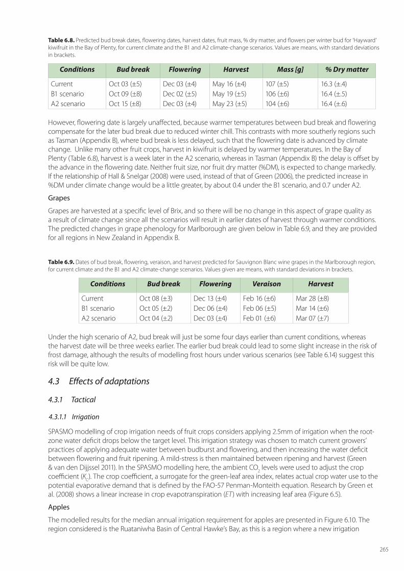
265

Table 6.8. Predicted bud break dates, flowering dates, harvest dates, fruit mass, % dry matter, and flowers per winter bud for ‘Hayward’ kiwifruit in the Bay of Plenty, for current climate and the B1 and A2 climate-change scenarios. Values are means, with standard deviations in brackets.

Conditions Bud break Flowering Harvest Mass [g] % Dry matter

CurrentB1 scenarioA2 scenario

Oct 03 (±5)Oct 09 (±8)Oct 15 (±8)

Dec 03 (±4)Dec 02 (±5)Dec 03 (±4)

May 16 (±4)May 19 (±5)May 23 (±5)

107 (±5)106 (±6)104 (±6)

16.3 (±.4)16.4 (±.5)16.4 (±.6)

However, flowering date is largely unaffected, because warmer temperatures between bud break and flowering compensate for the later bud break due to reduced winter chill. This contrasts with more southerly regions such as Tasman (Appendix B), where bud break is less delayed, such that the flowering date is advanced by climate change. Unlike many other fruit crops, harvest in kiwifruit is delayed by warmer temperatures. In the Bay of Plenty (Table 6.8), harvest is a week later in the A2 scenario, whereas in Tasman (Appendix B) the delay is offset by the advance in the flowering date. Neither fruit size, nor fruit dry matter (%DM), is expected to change markedly. If the relationship of Hall & Snelgar (2008) were used, instead of that of Green (2006), the predicted increase in %DM under climate change would be a little greater, by about 0.4 under the B1 scenario, and 0.7 under A2.

Grapes

Grapes are harvested at a specific level of Brix, and so there will be no change in this aspect of grape quality as a result of climate change since all the scenarios will result in earlier dates of harvest through warmer conditions. The predicted changes in grape phenology for Marlborough are given below in Table 6.9, and they are provided for all regions in New Zealand in Appendix B.

Table 6.9. Dates of bud break, flowering, veraison, and harvest predicted for Sauvignon Blanc wine grapes in the Marlborough region, for current climate and the B1 and A2 climate-change scenarios. Values given are means, with standard deviations in brackets.

Conditions Bud break Flowering Veraison Harvest

CurrentB1 scenarioA2 scenario

Oct 08 (±3)Oct 05 (±2)Oct 04 (±2)

Dec 13 (±4)Dec 06 (±4)Dec 03 (±4)

Feb 16 (±6)Feb 06 (±5)Feb 01 (±6)

Mar 28 (±8)Mar 14 (±6)Mar 07 (±7)

Under the high scenario of A2, bud break will just be some four days earlier than current conditions, whereas the harvest date will be three weeks earlier. The earlier bud break could lead to some slight increase in the risk of frost damage, although the results of modelling frost hours under various scenarios (see Table 6.14) suggest this risk will be quite low.

4.3 Effects of adaptations

4.3.1 Tactical

4.3.1.1 Irrigation

SPASMO modelling of crop irrigation needs of fruit crops considers applying 2.5mm of irrigation when the root-zone water deficit drops below the target level. This irrigation strategy was chosen to match current growers’ practices of applying adequate water between budburst and flowering, and then increasing the water deficit between flowering and fruit ripening. A mild-stress is then maintained between ripening and harvest (Green & van den Dijjssel 2011). In the SPASMO modelling here, the ambient CO2 levels were used to adjust the crop coefficient (KC). The crop coefficient, a surrogate for the green-leaf area index, relates actual crop water use to the potential evaporative demand that is defined by the FAO-57 Penman-Monteith equation. Research by Green et al. (2008) shows a linear increase in crop evapotranspiration (ET) with increasing leaf area (Figure 6.5).

Apples

The modelled results for the median annual irrigation requirement for apples are presented in Figure 6.10. The region considered is the Ruataniwha Basin of Central Hawke’s Bay, as this is a region where a new irrigation

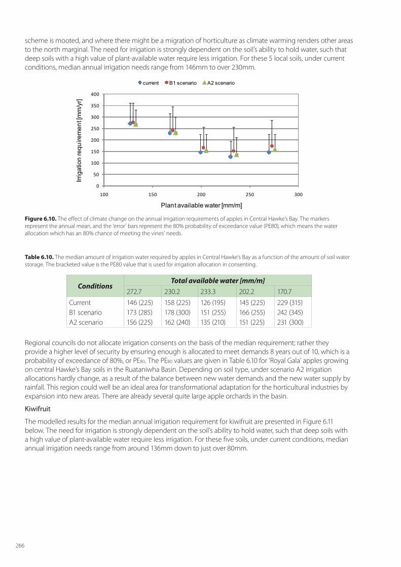
266

scheme is mooted, and where there might be a migration of horticulture as climate warming renders other areas to the north marginal. The need for irrigation is strongly dependent on the soil’s ability to hold water, such that deep soils with a high value of plant-available water require less irrigation. For these 5 local soils, under current conditions, median annual irrigation needs range from 146mm to over 230mm.

0

50

100

150

200

250

300

350

400

100 150 200 250 300

Irrig

atio

n re

quire

men

t [m

m/y

r]

Plant available water [mm/m]

current B1 scenario A2 scenario

Figure 6.10. The effect of climate change on the annual irrigation requirements of apples in Central Hawke’s Bay. The markers represent the annual mean, and the ‘error’ bars represent the 80% probability of exceedance value (PE80), which means the water allocation which has an 80% chance of meeting the vines’ needs.

Table 6.10. The median amount of irrigation water required by apples in Central Hawke’s Bay as a function of the amount of soil water storage. The bracketed value is the PE80 value that is used for irrigation allocation in consenting.

ConditionsTotal available water [mm/m]

272.7 230.2 233.3 202.2 170.7CurrentB1 scenarioA2 scenario

146 (225)173 (285)156 (225)

158 (225)178 (300)162 (240)

126 (195)151 (255)135 (210)

145 (225)166 (255)151 (225)

229 (315)242 (345)231 (300)

Regional councils do not allocate irrigation consents on the basis of the median requirement; rather they provide a higher level of security by ensuring enough is allocated to meet demands 8 years out of 10, which is a probability of exceedance of 80%, or PE80. The PE80 values are given in Table 6.10 for ‘Royal Gala’ apples growing on central Hawke’s Bay soils in the Ruataniwha Basin. Depending on soil type, under scenario A2 irrigation allocations hardly change, as a result of the balance between new water demands and the new water supply by rainfall. This region could well be an ideal area for transformational adaptation for the horticultural industries by expansion into new areas. There are already several quite large apple orchards in the basin.

Kiwifruit

The modelled results for the median annual irrigation requirement for kiwifruit are presented in Figure 6.11 below. The need for irrigation is strongly dependent on the soil’s ability to hold water, such that deep soils with a high value of plant-available water require less irrigation. For these five soils, under current conditions, median annual irrigation needs range from around 136mm down to just over 80mm.

267

0

50

100

150

200

250

300

350

0 50 100 150 200 250 300

Irrig

atio

n re

quire

men

t [m

m/y

r]

Plant available water [mm/m]

Series1 B1 scenario A2 scenario

Figure 6.11. The effect of climate change on the annual irrigation requirements of kiwifruit in the Bay of Plenty. The markers represent the annual average, and the ‘error bars’ represent the PE80 value which has an 80% probability of meeting the vines’ needs.

Table 6.11. The median amount of irrigation water required by kiwifruit in the Bay of Plenty as a function of the amount of soil water storage. The bracketed value is the PE80 value that is used for irrigation allocation in consenting.

ConditionsTotal available water [mm/m]

239.8 210.6 205.8 202.7 195.4 187.8 142CurrentB1 scenarioA2 scenario

81 (135)160 (240)175 (315)

81 (135)155 (240)171 (315)

84 (135)158 (240)177 (330)

99 (165)178 (270)196 (345)

108 (165)190 (255)203 (345)

105 (165)184 (255)201 (345)

136 (210)215 (285)236 (345)

The PE80 values are given in Table 6.11 for kiwifruit growing on the local soils of the Bay of Plenty. Depending upon soil type, under scenario A2 irrigation allocations of PE80 are likely to double; on the deeper soils they rise from 135mm to 315mm; and on soils of lower water-holding capacity they rise from 210mm to 345mm. These increases are as a result of the balance between the new pattern of water demands and the new arrangement of water supply by rainfall. It is still an open question as to whether this irrigation water will be available (Chapter 8).

As discussed above in Section 4.2.2, the application if HC is expected to maintain kiwifruit yields in the Bay of Plenty (McPherson et al. 2001). However, if HC is banned in the future (as is a real possibility) an important adaptation option will be finding other vine treatments which adequately increase flower numbers.

Grapes

The modelled results for the median annual irrigation requirement for grapes are presented in Figure 6.12. The need for irrigation is strongly dependent on the soil’s ability to hold water, such that deep soils with a high value of plant-available water require less irrigation. For these five soils, under current conditions, median annual irrigation needs range from around 130mm down to just over 10mm.

0

50

100

150

200

250

0 50 100 150 200

Irrig

atio

n re

quire

men

t [m

m/y

r]

Plant available water [mm/m]

current B1 scenario A2 scenario

Figure 6.12. The effect of climate change on the annual irrigation requirements of grapes in Marlborough. The markers represent the annual average, and the ‘error bars’ represent the PE80 value which has an 80% probability of meeting the vines’s needs.

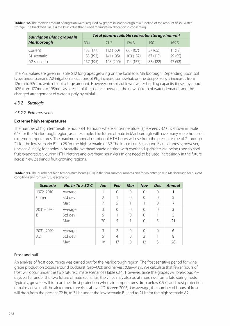
268

Table 6.12. The median amount of irrigation water required by grapes in Marlborough as a function of the amount of soil water storage. The bracketed value is the PE80 value that is used for irrigation allocation in consenting.

Sauvignon Blanc grapes in Marlborough

Total plant-available soil water storage [mm/m]

39.4 71.2 124.8 150 169.5

CurrentB1 scenarioA2 scenario

132 (177)153 (192)157 (195)

112 (160)141 (195)148 (200)

66 (107)103 (152)114 (157)

37 (65)67 (115)83 (122)

11 (12)29 (55)47 (52)

The PE80 values are given in Table 6.12 for grapes growing on the local soils Marlborough. Depending upon soil type, under scenario A2 irrigation allocations of PE80 increase somewhat; on the deeper soils it increases from 12mm to 52mm, which is not a large amount. However, on soils of lower water-holding capacity it rises by about 10% from 177mm to 195mm, as a result of the balance between the new pattern of water demands and the changed arrangement of water supply by rainfall.

4.3.2 Strategic

4.3.2.2 Extreme events

Extreme high temperatures

The number of high temperature hours (HTH) hours where air temperature (Ta) exceeds 32°C is shown in Table 6.13 for the Marlborough region, as an example. The future climate in Marlborough will have many more hours of extreme temperatures. The maximum annual number of HTH hours will rise from the present value of 7, through 21 for the low scenario B1, to 28 for the high scenario of A2 The impact on Sauvignon Blanc grapes is, however, unclear. Already, for apples in Australia, overhead shade netting with overhead sprinklers are being used to cool fruit evaporatively during HTH. Netting and overhead sprinklers might need to be used increasingly in the future across New Zealand’s fruit growing regions.

Table 6.13. The number of high temperature hours (HTH) in the four summer months and for an entire year in Marlborough for current conditions and for two future scenarios.

Scenario No. hr Ta > 32°C Jan Feb Mar Nov Dec Annual1972–2010Current

AverageStd devMax

127

015

001

001

000

127

2031–2070 B1

AverageStd devMax

35

20

015

001

000

015

35

21

2031–2070 A2

AverageStd devMax

3518

2417

000

0212

013

68

28

Frost and hail

An analysis of frost occurrence was carried out for the Marlborough region. The frost sensitive period for wine grape production occurs around budburst (Sep–Oct) and harvest (Mar–May). We calculate that fewer hours of frost will occur under the two future climate scenarios (Table 6.14). However, since the grapes will break bud 4-7 days earlier under the two future climate scenarios, the vines may also be at more risk from a late spring frosts. Typically, growers will turn on their frost protection when air temperatures drop below 0.5°C, and frost protection remains active until the air temperature rises above 4°C (Green 2006). On average, the number of hours of frost will drop from the present 72 hr, to 34 hr under the low scenario B1, and to 24 hr for the high scenario A2.

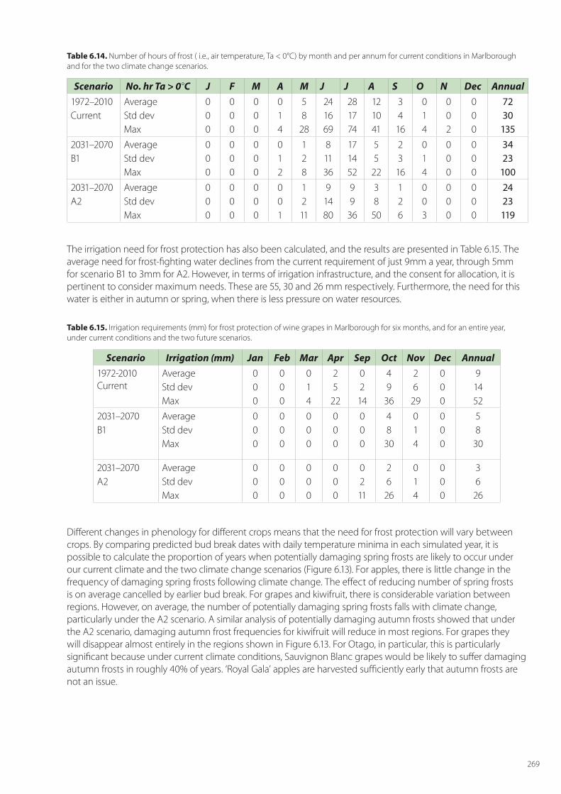
269

Table 6.14. Number of hours of frost ( i.e., air temperature, Ta < 0°C) by month and per annum for current conditions in Marlborough and for the two climate change scenarios.

Scenario No. hr Ta > 0°C J F M A M J J A S O N Dec Annual1972–2010Current

AverageStd devMax

000

000

000

014

58

28

241669

281774

121041

3416

014

002

000

7230135

2031–2070B1

AverageStd devMax

000

000

000

012

128

81136

171452

55

22

2316

014

000

000

3423

1002031–2070A2

AverageStd devMax

000

000

000

001

1211

91480

99

36

38

50

126

003

000

000

2423119

The irrigation need for frost protection has also been calculated, and the results are presented in Table 6.15. The average need for frost-fighting water declines from the current requirement of just 9mm a year, through 5mm for scenario B1 to 3mm for A2. However, in terms of irrigation infrastructure, and the consent for allocation, it is pertinent to consider maximum needs. These are 55, 30 and 26 mm respectively. Furthermore, the need for this water is either in autumn or spring, when there is less pressure on water resources.

Table 6.15. Irrigation requirements (mm) for frost protection of wine grapes in Marlborough for six months, and for an entire year, under current conditions and the two future scenarios.

Scenario Irrigation (mm) Jan Feb Mar Apr Sep Oct Nov Dec Annual1972-2010 Current

AverageStd devMax

000

000

014

25

22

0214

49

36

26

29

000

91452

2031–2070 B1

AverageStd devMax

000

000

000

000

000

48

30

014

000

58

30

2031–2070 A2

AverageStd devMax

000

000

000

000

0211

26

26

014

000

36

26

Different changes in phenology for different crops means that the need for frost protection will vary between crops. By comparing predicted bud break dates with daily temperature minima in each simulated year, it is possible to calculate the proportion of years when potentially damaging spring frosts are likely to occur under our current climate and the two climate change scenarios (Figure 6.13). For apples, there is little change in the frequency of damaging spring frosts following climate change. The effect of reducing number of spring frosts is on average cancelled by earlier bud break. For grapes and kiwifruit, there is considerable variation between regions. However, on average, the number of potentially damaging spring frosts falls with climate change, particularly under the A2 scenario. A similar analysis of potentially damaging autumn frosts showed that under the A2 scenario, damaging autumn frost frequencies for kiwifruit will reduce in most regions. For grapes they will disappear almost entirely in the regions shown in Figure 6.13. For Otago, in particular, this is particularly significant because under current climate conditions, Sauvignon Blanc grapes would be likely to suffer damaging autumn frosts in roughly 40% of years. ‘Royal Gala’ apples are harvested sufficiently early that autumn frosts are not an issue.

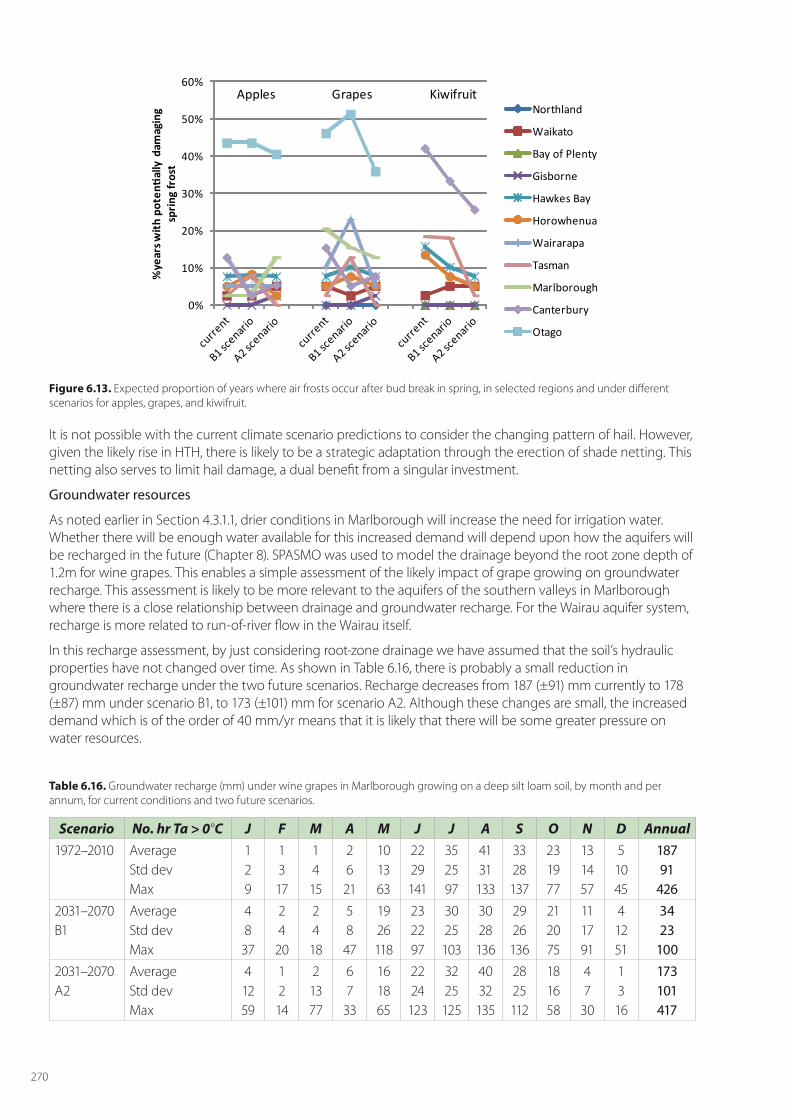
270

0%

10%

20%

30%

40%

50%

60%

%ye

ars w

ith p

oten

tially

dam

agin

g sp

ring

fros

t

Northland

Waikato

Bay of Plenty

Gisborne

Hawkes Bay

Horowhenua

Wairarapa

Tasman

Marlborough

Canterbury

Otago

Apples Grapes Kiwifruit

Figure 6.13. Expected proportion of years where air frosts occur after bud break in spring, in selected regions and under different scenarios for apples, grapes, and kiwifruit.

It is not possible with the current climate scenario predictions to consider the changing pattern of hail. However, given the likely rise in HTH, there is likely to be a strategic adaptation through the erection of shade netting. This netting also serves to limit hail damage, a dual benefit from a singular investment.

Groundwater resources

As noted earlier in Section 4.3.1.1, drier conditions in Marlborough will increase the need for irrigation water. Whether there will be enough water available for this increased demand will depend upon how the aquifers will be recharged in the future (Chapter 8). SPASMO was used to model the drainage beyond the root zone depth of 1.2m for wine grapes. This enables a simple assessment of the likely impact of grape growing on groundwater recharge. This assessment is likely to be more relevant to the aquifers of the southern valleys in Marlborough where there is a close relationship between drainage and groundwater recharge. For the Wairau aquifer system, recharge is more related to run-of-river flow in the Wairau itself.

In this recharge assessment, by just considering root-zone drainage we have assumed that the soil’s hydraulic properties have not changed over time. As shown in Table 6.16, there is probably a small reduction in groundwater recharge under the two future scenarios. Recharge decreases from 187 (±91) mm currently to 178 (±87) mm under scenario B1, to 173 (±101) mm for scenario A2. Although these changes are small, the increased demand which is of the order of 40 mm/yr means that it is likely that there will be some greater pressure on water resources.

Table 6.16. Groundwater recharge (mm) under wine grapes in Marlborough growing on a deep silt loam soil, by month and per annum, for current conditions and two future scenarios.

Scenario No. hr Ta > 0°C J F M A M J J A S O N D Annual1972–2010 Average

Std devMax

129

1317

1415

2621

101363

2229141

352597

4131133

3328137

231977

131457

51045

18791

4262031–2070B1

AverageStd devMax

4837

24

20

2418

5847

1926118

232297

3025103

3028136

2926136

212075

111791

41251

3423

1002031–2070A2

AverageStd devMax

41259

1214

21377

67

33

161865

2224

123

3225125

4032135

2825112

181658

47

30

1316

173101417

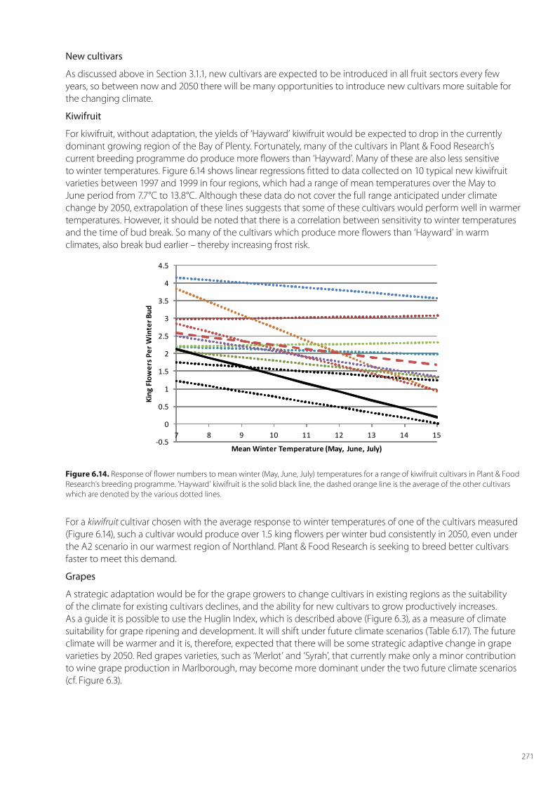
271

New cultivars

As discussed above in Section 3.1.1, new cultivars are expected to be introduced in all fruit sectors every few years, so between now and 2050 there will be many opportunities to introduce new cultivars more suitable for the changing climate.

Kiwifruit

For kiwifruit, without adaptation, the yields of ‘Hayward’ kiwifruit would be expected to drop in the currently dominant growing region of the Bay of Plenty. Fortunately, many of the cultivars in Plant & Food Research’s current breeding programme do produce more flowers than ‘Hayward’. Many of these are also less sensitive to winter temperatures. Figure 6.14 shows linear regressions fitted to data collected on 10 typical new kiwifruit varieties between 1997 and 1999 in four regions, which had a range of mean temperatures over the May to June period from 7.7°C to 13.8°C. Although these data do not cover the full range anticipated under climate change by 2050, extrapolation of these lines suggests that some of these cultivars would perform well in warmer temperatures. However, it should be noted that there is a correlation between sensitivity to winter temperatures and the time of bud break. So many of the cultivars which produce more flowers than ‘Hayward’ in warm climates, also break bud earlier – thereby increasing frost risk.

-0.5

0

0.5

1

1.5

2

2.5

3

3.5

4

4.5

7 8 9 10 11 12 13 14 15

King

Flo

wer

s Per

Win

ter B

ud

Mean Winter Temperature (May, June, July)

Figure 6.14. Response of flower numbers to mean winter (May, June, July) temperatures for a range of kiwifruit cultivars in Plant & Food Research’s breeding programme. ‘Hayward’ kiwifruit is the solid black line, the dashed orange line is the average of the other cultivars which are denoted by the various dotted lines.

For a kiwifruit cultivar chosen with the average response to winter temperatures of one of the cultivars measured (Figure 6.14), such a cultivar would produce over 1.5 king flowers per winter bud consistently in 2050, even under the A2 scenario in our warmest region of Northland. Plant & Food Research is seeking to breed better cultivars faster to meet this demand.

Grapes

A strategic adaptation would be for the grape growers to change cultivars in existing regions as the suitability of the climate for existing cultivars declines, and the ability for new cultivars to grow productively increases. As a guide it is possible to use the Huglin Index, which is described above (Figure 6.3), as a measure of climate suitability for grape ripening and development. It will shift under future climate scenarios (Table 6.17). The future climate will be warmer and it is, therefore, expected that there will be some strategic adaptive change in grape varieties by 2050. Red grapes varieties, such as ‘Merlot’ and ‘Syrah’, that currently make only a minor contribution to wine grape production in Marlborough, may become more dominant under the two future climate scenarios (cf. Figure 6.3).

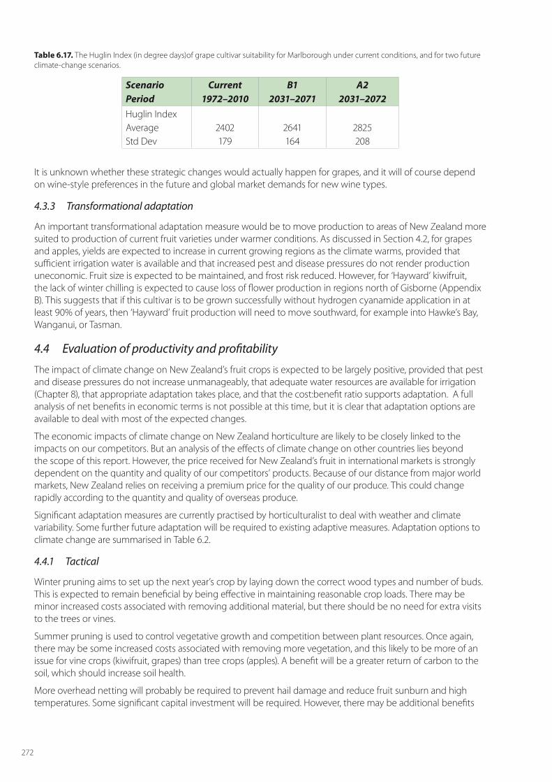
272

Table 6.17. The Huglin Index (in degree days)of grape cultivar suitability for Marlborough under current conditions, and for two future climate-change scenarios.

ScenarioPeriod

Current1972–2010

B1 2031–2071

A2 2031–2072

Huglin IndexAverageStd Dev

2402179

2641164

2825208

It is unknown whether these strategic changes would actually happen for grapes, and it will of course depend on wine-style preferences in the future and global market demands for new wine types.

4.3.3 Transformational adaptation

An important transformational adaptation measure would be to move production to areas of New Zealand more suited to production of current fruit varieties under warmer conditions. As discussed in Section 4.2, for grapes and apples, yields are expected to increase in current growing regions as the climate warms, provided that sufficient irrigation water is available and that increased pest and disease pressures do not render production uneconomic. Fruit size is expected to be maintained, and frost risk reduced. However, for ‘Hayward’ kiwifruit, the lack of winter chilling is expected to cause loss of flower production in regions north of Gisborne (Appendix B). This suggests that if this cultivar is to be grown successfully without hydrogen cyanamide application in at least 90% of years, then ‘Hayward’ fruit production will need to move southward, for example into Hawke’s Bay, Wanganui, or Tasman.

4.4 Evaluation of productivity and profitability

The impact of climate change on New Zealand’s fruit crops is expected to be largely positive, provided that pest and disease pressures do not increase unmanageably, that adequate water resources are available for irrigation (Chapter 8), that appropriate adaptation takes place, and that the cost:benefit ratio supports adaptation. A full analysis of net benefits in economic terms is not possible at this time, but it is clear that adaptation options are available to deal with most of the expected changes.

The economic impacts of climate change on New Zealand horticulture are likely to be closely linked to the impacts on our competitors. But an analysis of the effects of climate change on other countries lies beyond the scope of this report. However, the price received for New Zealand’s fruit in international markets is strongly dependent on the quantity and quality of our competitors’ products. Because of our distance from major world markets, New Zealand relies on receiving a premium price for the quality of our produce. This could change rapidly according to the quantity and quality of overseas produce.

Significant adaptation measures are currently practised by horticulturalist to deal with weather and climate variability. Some further future adaptation will be required to existing adaptive measures. Adaptation options to climate change are summarised in Table 6.2.

4.4.1 Tactical

Winter pruning aims to set up the next year’s crop by laying down the correct wood types and number of buds. This is expected to remain beneficial by being effective in maintaining reasonable crop loads. There may be minor increased costs associated with removing additional material, but there should be no need for extra visits to the trees or vines.

Summer pruning is used to control vegetative growth and competition between plant resources. Once again, there may be some increased costs associated with removing more vegetation, and this likely to be more of an issue for vine crops (kiwifruit, grapes) than tree crops (apples). A benefit will be a greater return of carbon to the soil, which should increase soil health.

More overhead netting will probably be required to prevent hail damage and reduce fruit sunburn and high temperatures. Some significant capital investment will be required. However, there may be additional benefits

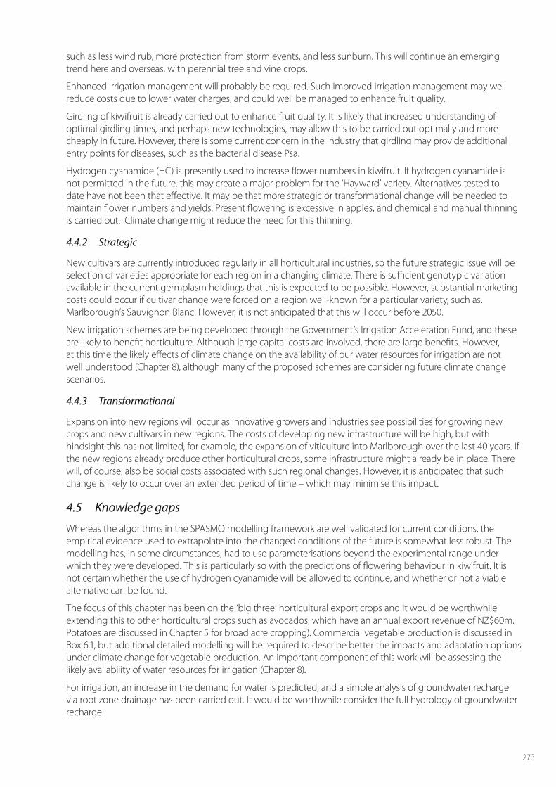
273

such as less wind rub, more protection from storm events, and less sunburn. This will continue an emerging trend here and overseas, with perennial tree and vine crops.

Enhanced irrigation management will probably be required. Such improved irrigation management may well reduce costs due to lower water charges, and could well be managed to enhance fruit quality.

Girdling of kiwifruit is already carried out to enhance fruit quality. It is likely that increased understanding of optimal girdling times, and perhaps new technologies, may allow this to be carried out optimally and more cheaply in future. However, there is some current concern in the industry that girdling may provide additional entry points for diseases, such as the bacterial disease Psa.

Hydrogen cyanamide (HC) is presently used to increase flower numbers in kiwifruit. If hydrogen cyanamide is not permitted in the future, this may create a major problem for the ‘Hayward’ variety. Alternatives tested to date have not been that effective. It may be that more strategic or transformational change will be needed to maintain flower numbers and yields. Present flowering is excessive in apples, and chemical and manual thinning is carried out. Climate change might reduce the need for this thinning.

4.4.2 Strategic

New cultivars are currently introduced regularly in all horticultural industries, so the future strategic issue will be selection of varieties appropriate for each region in a changing climate. There is sufficient genotypic variation available in the current germplasm holdings that this is expected to be possible. However, substantial marketing costs could occur if cultivar change were forced on a region well-known for a particular variety, such as. Marlborough’s Sauvignon Blanc. However, it is not anticipated that this will occur before 2050.

New irrigation schemes are being developed through the Government’s Irrigation Acceleration Fund, and these are likely to benefit horticulture. Although large capital costs are involved, there are large benefits. However, at this time the likely effects of climate change on the availability of our water resources for irrigation are not well understood (Chapter 8), although many of the proposed schemes are considering future climate change scenarios.

4.4.3 Transformational

Expansion into new regions will occur as innovative growers and industries see possibilities for growing new crops and new cultivars in new regions. The costs of developing new infrastructure will be high, but with hindsight this has not limited, for example, the expansion of viticulture into Marlborough over the last 40 years. If the new regions already produce other horticultural crops, some infrastructure might already be in place. There will, of course, also be social costs associated with such regional changes. However, it is anticipated that such change is likely to occur over an extended period of time – which may minimise this impact.

4.5 Knowledge gaps

Whereas the algorithms in the SPASMO modelling framework are well validated for current conditions, the empirical evidence used to extrapolate into the changed conditions of the future is somewhat less robust. The modelling has, in some circumstances, had to use parameterisations beyond the experimental range under which they were developed. This is particularly so with the predictions of flowering behaviour in kiwifruit. It is not certain whether the use of hydrogen cyanamide will be allowed to continue, and whether or not a viable alternative can be found.

The focus of this chapter has been on the ‘big three’ horticultural export crops and it would be worthwhile extending this to other horticultural crops such as avocados, which have an annual export revenue of NZ$60m. Potatoes are discussed in Chapter 5 for broad acre cropping). Commercial vegetable production is discussed in Box 6.1, but additional detailed modelling will be required to describe better the impacts and adaptation options under climate change for vegetable production. An important component of this work will be assessing the likely availability of water resources for irrigation (Chapter 8).

For irrigation, an increase in the demand for water is predicted, and a simple analysis of groundwater recharge via root-zone drainage has been carried out. It would be worthwhile consider the full hydrology of groundwater recharge.

274

5 Summary

Many of the anticipated impacts of climate change on these fruit crops are positive. These include increased, or at least not decreased, yields, fruit size, and fruit dry matter. There will be reduced, or at least not increased, risk of frost damage. However, adaptation will be required to deal with some potentially negative impacts. These include reduced flower numbers in kiwifruit; increased water use by all crops; increased pest and disease pressure; more extreme high temperatures, and a probable increase in storm damage through wind and hail.

Horticultural production is highly managed and presently many interventions, or adaptations, are used to encourage the production of high-quality and fit-for-purpose fruit and berries. Tactical adaptations are standard practice, such as irrigation, the use of chemical thinning, trimming, pruning and flower inducing sprays. These will easily be modified and employed to enable tactical adaptation to climate change by 2050.

There are already many strategic adaptations in use, such as the introduction of new cultivars and infrastructural investments in overhead netting for hail protection and shading.

The horticultural industry, especially viticulture, is nimble, and it has shown that it can undergo transformational change in response to economic opportunities. The rise in the planted area of vineyards in New Zealand in general, and Marlborough in particular, highlights this. If the transformational change of seeking new regions in which to grow existing crops is brought about by climate change, then it is likely this will occur: competition for land and water notwithstanding.

6 ReferencesAinsworth, E.A.; Rogers, A. (2007). The response of photosynthesis and stomatal conductance to rising [CO2]: mechanisms and environmental interactions. Plant, Cell and Environment 30(3): 258–270.

Aurambout, J-P.; Constable, F.; Luck, J.; Sposito, V. (2006). The impacts of climate change on plant biosecurity – literature review. Department of Primary Industries and Cooperative Research Centre for Plant Biosecurity, Melbourne.

Austin, P.T.; Hall, A.J. (2001). Climate change and development of apple fruits. Chapter 5 in: The Effects of Climate Change and Variability in New Zealand: An Assessment Using the CLIMPACTS System, Kenny, G.J.; Warrick, R.A.; Harman, J. (Eds.), IGCI, University of Waikato, Hamilton, New Zealand.

Austin, P.T.; Hall, A.J.; Gandar, P.W.; Warrington, I.J. Fulton, T.A.; Halligan, E.A. (1999). A compartment model of the effect of early-season temperatures on potential size and growth of ‘Delicious’ apple fruits. Annals of Botany 83: 129–143.

Baker, D.N.; Enoch, H.Z. (1983). Plant growth and development. In Lemon, E R (Ed) CO2 and Plants: The response of plants to rising levels of atmospheric carbon dioxide. Westview Press & AAAS, pp-107–130.

Bazzaz, F.A.; Miao, S.L.; Wayne, P.M. (1993). CO2 –induced growth enhancements of co-oocuring tree species decline at different rates. Oecologia 96: 478–482.

Bebbington, M.; Hall, A.J.; Lai, C.D.; Zitikis, R. (2009). Dynamics and phases of kiwifruit (Actinidia deliciosa) growth curves. New Zealand Journal Crop & Horticultural Science 37: 179–188.

Bindi, M.; Fibbi, L.; Gozzlni, B.; Orlandini, S.; Miglietta, F. (1995). Experiments on the effects of increased temperature and/or elevated concentrations of carbon dioxide on crops mini Free Air Carbon dioxide Enrichment (FACE) experiment on grapevine. In: Harrison, P.A.; Butterfield, R.E.; Downing, T.E. (eds) Climate change and agriculture in Europe: assessment of impacts and adaptations. Research Report No. 9, Environmental Change Unit, University of Oxford, pp. 125–137.

Bindi, M.; Fibbi, L.; Gozzlni, B.; Orlandini, S.; Miglietta, F. (1996). Modelling the impact of future scenarios on yield and yield variation of grapevines. Climate. Research. 7: 213–224.

Bunce, J.A. (1992). Stomatal conductance, photosynthesis and respiration of temperate deciduous tree seedlings grown outdoors at an elevated concentration of carbon dioxide. Plant Cell Environment. 15: 541–549.

Chuine, I.; Yiou, P.; Viovy, N.; Seguin, B.; Daux, V.; Le Roy Ladurie, E. (2004). Grape ripening as a past climate indicator. Nature 432: 289–290.

Clothier, B.E.; Green, S.R.; Deurer, M. (2008). Land management: The upper-boundary control on groundwater quality. In Securing Groundwater Quality in Urban and Industrial Environments, Proceedings 6th International Association for Hydrological Sciences, Groundwater Quality 2007, Fremantle, Western Australia, 2-7 December 2007 IAHS Publication (Ed. Michael Trefry) 324: 39–46.

Coakley, S.M.; Scherm, H.; Chakraborty, S. (1999). Climate change and plant disease management. Annual Review of Phytopathology 37: 399–426.

Cure, J.D. and Acock, B. 1986. Crop responses to carbon dioxide doubling: A literature survey. Agric. Forest. Meteorol. 38: 127–145.

Darbyshire, R.; Webb, L.; Goodwin, I.; Barlow, S. (2011). Winter chilling trends for deciduous fruit trees in Australia. Agricultural. Forest Meteorology. 151: 1074–1085.

Daymond, A.J.; Wheeler, T.R.; Hadley, P.; Ellis, R.H.; Morison, J.I.L. (1997). The growth, development and yield of onion (Allium cepa L.) in response to temperatue and CO2. Journal Horticultural Science. 72: 135–145.

Deurer, M.; Green, S.R.; Clothier, B.E.; Mowat, A. (2011). Can product water footprints indicate the hydrological impact of primary

275

production? – A case study of New Zealand kiwifruit. Journal of Hydrology 408(3-4): 2346–256.

Deurer, M.; Grinev, D.; Young, I.; Clothier, B.E.; Müller, K. (2009). The impact of soil carbon management on soil macro-pore structure: A comparison of two apple orchard systems in New Zealand. European Journal of Soil Science 60: 945–955.

Deuter, P.L. (1989). The development of an insecticide resistance strategy for the Lockyer Valley, Queensland. Acta Horticulturae. 247: 267–272.

Dioguardi, D. (1995). Lettuces. In: B. Coombes (ed). Horticulture Australia. Morescope Publishing, Hawthorn, Vic. Australia.

Drake, B.G.; Gonzales-Meler, M.A.; Long, S.P. (1997). More efficient plants: a consequence of rising CO2. Annual review of Plant Physiology and Molecular Biology 48: 609–639.

Fresh Facts. (2011). Fresh Facts: New Zealand Horticulture. New Zealand Institute for Plant & Food Research Ltd., Auckland, New Zealand, 32 p.

Gerard, P.J.; Kean, J.M.; Phillips, C.B.; Fowler, S.V.; Withers, T.M.; Walker, G.P.; Charles, J.G. (2010). Possible impacts of climate change on biocontrol systems in New Zealand. Report for MAF Pol Project 0910-11689, Client report number: SC110/2010/170.

Girona, J.; Mata, M.; del Campo, J.; Arbonés, A.; Barta, E.; Marsal, J. (2006). The use of midday leaf water potential for scheduling deficit irrigation in vineyards. Irrigation Science 24: 115–127.

Green, S.R. (2006). Waihopai Valley Vintners – Water Allocation Assessment . A report prepared for Waihopai Valley Vintners Ltd. PFR Client Report.

Green, S.R. (2007). Kiwifruit dry matter platform – exploiting water stress using summer deficit irrigation. Component A: Feasibility evaluation. Report to ZESPRI Group Limited. HortResearch Client Report.

Green, S.R; Agnew, R.; Greven, M. (2009). Irrigation trials on grapevines in the Lower Awatere Valley – Marlborough. A report prepared for Marlborough District Council. Plant & Food Research, Report No 2756.

Green, S.R.; Clothier, B.E. (1995). Root-water uptake by kiwifruit vines following partial wetting of the root zone. Plant and Soil 173: 317–328.

Green, S.R.; Clothier, B.E. (1999). The rootzone dynamics of water uptake by a mature apple tree Plant and Soil 206: 61–77.

Green, S.R.; Clothier, B.E.; McLeod, D.J. (1997). The response of sap flow in apple roots to localised irrigation. Agricultural Water Management 33: 63–78.

Green, S.R.; Clothier, B.E.; Mills, T.M.; Millar, A. (1999). Risk assessment of the irrigation requirements for field crops in a maritime climate. Journal of Crop Production 2(2): 353–377.

Green, S.R.; Clothier, B.E.; van den Dijssel, C.; Deurer, M.; Davidson, P. (2008). Measurement and modelling the stress response of grapevines to soil-water deficits in their rootzones. Chapter 15, In Soil Science Society America Monograph ‘Modeling the response of crops to limited water: Recent advances in understanding and modeling water stress effects on plant growth processes’, Ahuja, L. et al. (eds) pp. 357–386.

Green, S.R.; Kirkham, M.B.; Clothier, B.E. (2006). Root uptake and transpiration: From measurements and models to sustainable irrigation. Agricultural Water Management 86: 165–176.

Green, S.R.; van den Dijssel, C. (2011). Ground-water abstraction from the Wairau Plains. A report prepared for Marlborough District Council. PFR Client Report No 5923.

Green, S.R.; Vogeler, I.; Clothier, B.E.; Mills, T.M.; van den Dijssel, C. (2002). Modelling water uptake by a mature apple tree. Australian Journal of Soil Research 41: 365–380.

Hall, A.J.; Kenny, G.J.; Austin, P.T.; McPherson, H.G. (2001). Changes in kiwifruit phenology with climate. Chapter 4 in: The Effects of Climate Change and Variability in New Zealand: An Assessment Using the CLIMPACTS System, Kenny, G.J.; Warrick, R.A.; Harman, J. (Eds.), IGCI, University of Waikato, Hamilton, New Zealand.

Hall, A.J.; McPherson, H.G. (1997a). Modelling the influence of temperature on the timing of bud break in kiwifruit. Acta Horticulturae 444: 401–406.

Hall, A.J.; McPherson, H.G. (1997b). Predicting fruit maturation in kiwifruit (Actinidia deliciosa). Journal of Horticultural Science 72(6): 949–960.

Hall, A.J.; Minchin, P.E.H.; Snelgar, W.P. (2002). Using scaled growth curves to make predictions: pitfalls and solutions. Acta Horticulturae 584:133–139.

Hall, A.J.; Snelgar, W.P. (2008). Temperature effects on kiwifruit dry matter at harvest. Acta Horticulturae 803: 155–162.

Hartz, T.K.; Baameur, A., Holt, D.B. (1991). Carbon dioxide enrichment of high value crops under tunnel culture. Journal American Horticultural Science. 26: 970–973.

Hennessey, K.J.; Clayton-Greene, K. (1995). Greenhouse warming and veranalisation of high-chill fruit in Southern Australia Climate Change 30: 327–348.

Huglin, P. (1978). Nouveau mode d’évaluation des possibilités héliothermiques de la vigne. C.R. Acad. Agric. Fr.1117-1126.

Idso, S.B.; Kimball, B.A.; Allen, S.G. (1991). CO2 enrichment of sour orange trees: 2.5 years into a long-term experiment Plant Cell Environ. 14: 351–353.

Kenny, G. (2001). Climate Change: likely impacts on New Zealand Agriculture. A report prepared for the Ministry for the Environment.

Kenny, G. (2008). Adapting to climate change in the kiwifruit industry. A report prepared for MAF June 2008.

Kimball, B.A., Kobayashi, K., Bindi, M. (2002). Responses of agricultural crops to free-air CO2 enrichment. Advances in Agronomy 77: 293–368.

276

Kimball, B.A., Idso, S.B.; Johnson, S., Rillig, M.C. (2007). Seventeen years of carbon dioxide enrichment of sour orange trees. Global Change Biology. 13: 2171–2183.

Kirkham, M.B. (2011). Elevated Carbon Dioxide: Impacts on Soil and Plant Water Relations.CRC Press, 399 p.

Maltby, J.E. (1995). Tomatoes. In: B. Coombes Ed. Horticulture Australia. Morescope Publishing, Hawthorn, Vic., Australia.

Matamala, R.; Gonzalez-Meler, M.A.; Jastrow, J.D.; Norby, R.J.; Schlesinger, W.H. (2003). Impacts of fine root turnover on forest NPP and soil C sequestration potential. Science 302: 1385–1387.

Miller, S.A.; Smith, G.S.; Boldingh, H.L.; Johansson, A. (1998). Effects of Water Stress on Fruit Quality Attributes of Kiwifruit. Annals of Botany 81: 73–81.

Monk, P.R.; Hook D.; Freeman, B.M. (1986). Amino acid metabolism in yeasts. In: Lee, T. (ed.) Proceedings of the Sixth Wine Industry Technical Conference, 14–17 July, Adelaide, SA.

Murray, D.R. (1997). Carbon Dioxide and Plant Responses John Wiley & Sons, 275 p.

McPherson, H.G.; Hall, A.J.; Stanley, C.J. (1992). The influence of current temperature on the time from bud break to flowering in kiwifruit (Actinidia deliciosa). Journal of Horticultural Science 67: 509–519.

McPherson, H.G.; Richardson, A.C.; Snelgar, W.P.; Currie, M.B. (2001). Effects of hydrogen cyanamide on budbreak and flowering in kiwifruit (Actinidia deliciosa

‘Hayward’). New Zealand Journal of Crop & Horticultural Science 29: 277–285.

Mpelasoka, B.S.; Behboudian, M.H.; Mills, T.M. (2001). Effects of deficit irrigation on fruit maturity and quality of ‘Braeburn’ apple. Scientia Horticulturae 90: 279–290.

Nederhoff, E.M.; Buitelaar, K. (1992). Effects of CO2 on greenhouse grown eggplants (Solanum melongena L.) II Leaf tip chlorosis and fruit production. J. Hort. Sci. 67: 805–812.

Palmer, J.W.; Guiliani, R.; Adams, H.M. (1997). Effect of crop load on fruiting and leaf photosynthesis of ‘Braeburn’/M.26 apple trees. Tree Physiology 17: 741–746.

Palmer, J.W.; Harker, F.R.; Tustin, D.S.; Johnstone, J. (2010). Fruit dry matter concentration: A new quality metric for apples. Journal of the Science of Food and. Agriculture. 15: 2586–94.

Parker, A.K.; De Cortázar-Atauri, I.G.; Van Leeuwen, C.; Chuine, I. (2011). General phenological model to characterise the timing of flowering and veraison of Vitis vinifera L. Australian Journal of Grape and Wine Research 17(2): 206–216

Pearson, S.; Wheeler, T.R.; Hadley, P.; Wheldon, A.E. (2007). A validated model to predict the effects of environment on the growth of lettuce (Lactuca sativa L.): Implications for climate change. Journal of Horticultural Science. 72: 503–517.

Putland, D.; Deuter, P.; Hayman, P.; Hetherington. S.; Middleton, S.; Nidumolu, U.; Nimmo, P.; Thomas, D.; Wilkie, J.; Williams, D. (2011). The apple and pear industry’s response to climate change and variability: A desktop study. Australian Fruitgrower – August 2011. (HAL Project Report AP09019): 14–17.

Reddy, K.R.; Hodges, H.F.; McKinion, J.M. (1992). Cotton crop response to global climate change World Resource Rev. 4: 348–365.

Richardson, A.C.; McAneney, K.J. (1990). Influence of fruit number on fruit weight and yield in kiwifruit. Scientia Horticulturae 42: 233–241.

Richardson, A.C.; Marsh, K.B.; Boldingh, H.L.; Pickering, A.H.; Bulley, S.M.; Frearson, N.J.; Ferguson, A.R.; Thornber, S.E.; Bolitho, K.M.; Macrae, E.A. (2004). High growing temperatures reduce fruit carbohydrate and vitamin C in kiwifruit. Plant, Cell, and Environment 27(4): 423–435.

Schulman, Y.; Nir, G.; Fanberstein, L.; Lavee, S. (1983). The effect of cyanamide on the release from dormancy of grapevine buds. Scientia Horticulturae 19: 97–104.

Seguin, B.; Garcia de Cortazar, I. (2005). Climate Warming: Consequences for viticulture and the notion of ‘terroir’ in Europe. Acta Hort. 689:61–70.

Snelgar, W.P.; Hall, A.J.; McPherson, H.G. (2008). Modelling flower production of kiwifruit (Actinidia deliciosa) from Winter chilling. NZ Journal of Crop and Horticultural Science 36(4): 273–284.

Snelgar, W.P.; Hall, A.J.; Richardson, A.C.; Currie, M.B. (2007). Influence of temperature on between-season variation in dry matter content of ‘hayward’ kiwifruit. Acta Horticulturae. 753: 383–388.

Stanley, C.J.; Tustin, D.S.; Lupton, G.B.; McArtney, S.; Cashmore, W.M.; De Silva, H.N. (2000). Towards understanding the role of temperature in apple fruit growth responses in three geographical regions within New Zealand. Journal of Horticultural Science and Biotechnology 75(4).

Stokes, C.; Howden, M. (2010). Adapting agriculture to climate change: preparing Australian Agriculture, Forestry and Fisheries for the Future, CSIRO Publishing, 296 p.

Tait, A.B. (2008). Future projections of growing degree days and frost in New Zealand and some implications for grape growing. Weather and Climate 28: 17–36.

Tingey, D.J.; Johnson, M.G.; Phillips, D.C. (2005). Independent and contrasting effects of elevated CO2 and N fertilization on root architecture of Pinus ponderosa. Trees – Structure and Function 19:43–50.

Trought, M.C.T. (2005). Fruitset – possible implications on wine quality. AVSO proceedings, Transforming Flowers to Fruit Workshop, Mildura, Australia, 32–36.

Webb, L.; Whetton, P.H. (2010). Horticulture. In: Stokes, C.J.; Howden, S.M. (Eds) Adapting Australian Agricul;ture to Climate Change. pp 119–136. CSIRO Publishing, Collingwood, Australia.

Wünsche, J.N.; Bown, J.; Ferguson, I.; Woolf, A.; McGhie, T. (2004). Sunburn on apples – Causes and controls mechanisms. Acta Horticulturae 636: 631–636.

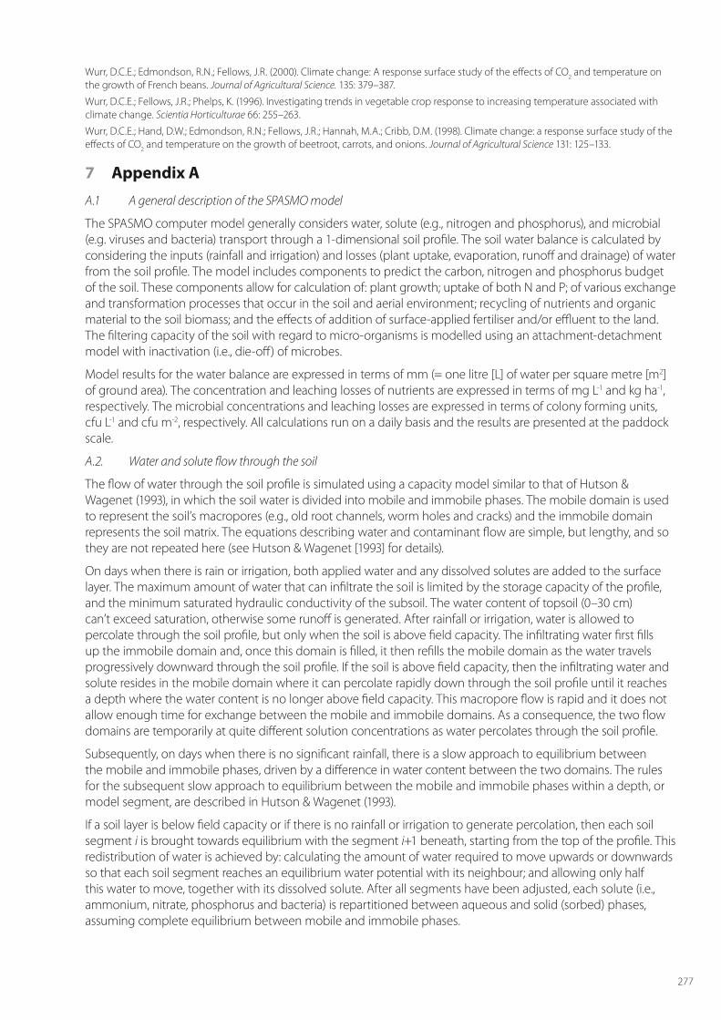
277

Wurr, D.C.E.; Edmondson, R.N.; Fellows, J.R. (2000). Climate change: A response surface study of the effects of CO2 and temperature on the growth of French beans. Journal of Agricultural Science. 135: 379–387.

Wurr, D.C.E.; Fellows, J.R.; Phelps, K. (1996). Investigating trends in vegetable crop response to increasing temperature associated with climate change. Scientia Horticulturae 66: 255–263.

Wurr, D.C.E.; Hand, D.W.; Edmondson, R.N.; Fellows, J.R.; Hannah, M.A.; Cribb, D.M. (1998). Climate change: a response surface study of the effects of CO2 and temperature on the growth of beetroot, carrots, and onions. Journal of Agricultural Science 131: 125–133.

7 Appendix A

A.1 A general description of the SPASMO model

The SPASMO computer model generally considers water, solute (e.g., nitrogen and phosphorus), and microbial (e.g. viruses and bacteria) transport through a 1-dimensional soil profile. The soil water balance is calculated by considering the inputs (rainfall and irrigation) and losses (plant uptake, evaporation, runoff and drainage) of water from the soil profile. The model includes components to predict the carbon, nitrogen and phosphorus budget of the soil. These components allow for calculation of: plant growth; uptake of both N and P; of various exchange and transformation processes that occur in the soil and aerial environment; recycling of nutrients and organic material to the soil biomass; and the effects of addition of surface-applied fertiliser and/or effluent to the land. The filtering capacity of the soil with regard to micro-organisms is modelled using an attachment-detachment model with inactivation (i.e., die-off) of microbes.

Model results for the water balance are expressed in terms of mm (= one litre [L] of water per square metre [m2] of ground area). The concentration and leaching losses of nutrients are expressed in terms of mg L-1 and kg ha-1, respectively. The microbial concentrations and leaching losses are expressed in terms of colony forming units, cfu L-1 and cfu m-2, respectively. All calculations run on a daily basis and the results are presented at the paddock scale.

A.2. Water and solute flow through the soil

The flow of water through the soil profile is simulated using a capacity model similar to that of Hutson & Wagenet (1993), in which the soil water is divided into mobile and immobile phases. The mobile domain is used to represent the soil’s macropores (e.g., old root channels, worm holes and cracks) and the immobile domain represents the soil matrix. The equations describing water and contaminant flow are simple, but lengthy, and so they are not repeated here (see Hutson & Wagenet [1993] for details).

On days when there is rain or irrigation, both applied water and any dissolved solutes are added to the surface layer. The maximum amount of water that can infiltrate the soil is limited by the storage capacity of the profile, and the minimum saturated hydraulic conductivity of the subsoil. The water content of topsoil (0–30 cm) can’t exceed saturation, otherwise some runoff is generated. After rainfall or irrigation, water is allowed to percolate through the soil profile, but only when the soil is above field capacity. The infiltrating water first fills up the immobile domain and, once this domain is filled, it then refills the mobile domain as the water travels progressively downward through the soil profile. If the soil is above field capacity, then the infiltrating water and solute resides in the mobile domain where it can percolate rapidly down through the soil profile until it reaches a depth where the water content is no longer above field capacity. This macropore flow is rapid and it does not allow enough time for exchange between the mobile and immobile domains. As a consequence, the two flow domains are temporarily at quite different solution concentrations as water percolates through the soil profile.

Subsequently, on days when there is no significant rainfall, there is a slow approach to equilibrium between the mobile and immobile phases, driven by a difference in water content between the two domains. The rules for the subsequent slow approach to equilibrium between the mobile and immobile phases within a depth, or model segment, are described in Hutson & Wagenet (1993).

If a soil layer is below field capacity or if there is no rainfall or irrigation to generate percolation, then each soil segment i is brought towards equilibrium with the segment i+1 beneath, starting from the top of the profile. This redistribution of water is achieved by: calculating the amount of water required to move upwards or downwards so that each soil segment reaches an equilibrium water potential with its neighbour; and allowing only half this water to move, together with its dissolved solute. After all segments have been adjusted, each solute (i.e., ammonium, nitrate, phosphorus and bacteria) is repartitioned between aqueous and solid (sorbed) phases, assuming complete equilibrium between mobile and immobile phases.

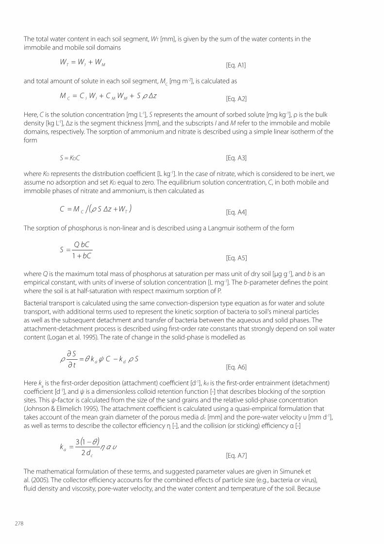
278

The total water content in each soil segment, WT [mm], is given by the sum of the water contents in the immobile and mobile soil domains

MIT WWW += [Eq. A1]

and total amount of solute in each soil segment, MC [mg m-2], is calculated as

zSWCWCM MMIIC ∆++= ρ [Eq. A2]

Here, C is the solution concentration [mg L-1], S represents the amount of sorbed solute [mg kg-1], ρ is the bulk density [kg L-1], ∆z is the segment thickness [mm], and the subscripts I and M refer to the immobile and mobile domains, respectively. The sorption of ammonium and nitrate is described using a simple linear isotherm of the form

S = KDC [Eq. A3]

where KD represents the distribution coefficient [L kg-1]. In the case of nitrate, which is considered to be inert, we assume no adsorption and set KD equal to zero. The equilibrium solution concentration, C, in both mobile and immobile phases of nitrate and ammonium, is then calculated as

( )TC WzSMC +∆= ρ [Eq. A4]

The sorption of phosphorus is non-linear and is described using a Langmuir isotherm of the form

bCbCQ

S+

=1

[Eq. A5]

where Q is the maximum total mass of phosphorus at saturation per mass unit of dry soil [µg g-1], and b is an empirical constant, with units of inverse of solution concentration [L mg-1]. The b-parameter defines the point where the soil is at half-saturation with respect maximum sorption of P.

Bacterial transport is calculated using the same convection-dispersion type equation as for water and solute transport, with additional terms used to represent the kinetic sorption of bacteria to soil’s mineral particles as well as the subsequent detachment and transfer of bacteria between the aqueous and solid phases. The attachment-detachment process is described using first-order rate constants that strongly depend on soil water content (Logan et al. 1995). The rate of change in the solid-phase is modelled as

SkCktS

da ρψθρ −=∂∂

[Eq. A6]

Here ka is the first-order deposition (attachment) coefficient [d-1], kd is the first-order entrainment (detachment) coefficient [d-1], and ψ is a dimensionless colloid retention function [-] that describes blocking of the sorption sites. This ψ-factor is calculated from the size of the sand grains and the relative solid-phase concentration (Johnson & Elimelich 1995). The attachment coefficient is calculated using a quasi-empirical formulation that takes account of the mean grain diameter of the porous media dc [mm] and the pore-water velocity υ [mm d-1], as well as terms to describe the collector efficiency η [-], and the collision (or sticking) efficiency α [-]

( )υαη

θ

ca d

k213 −

= [Eq. A7]

The mathematical formulation of these terms, and suggested parameter values are given in Simunek et al. (2005). The collector efficiency accounts for the combined effects of particle size (e.g., bacteria or virus), fluid density and viscosity, pore-water velocity, and the water content and temperature of the soil. Because

279

attachment is (approximately) inversely proportional to the grain size of the soil particles, finer grained soils such as silts and clays tend to be more efficient at trapping bacteria that are transported with the drainage waters. Furthermore, the smaller sized microbes (i.e., viruses as opposed to bacteria) are less likely to be intercepted by the soil particles (i.e. have a smaller collector efficiency), so the relative value of ka is reduced. For the purpose of modelling, the ratio ka/kd has been set to a constant value of 100. Other parameters used in modelling bacterial (i.e. E. coli) transport through the soil are discussed in Appendix B.

A.3. Calculation of crop water use

A standard crop-factor approach is used to relate crop water use to the prevailing weather and physiological time of development. The procedure is based on guidelines given by the Food and Agriculture Administration (FAO) of the United Nations (Allen et al. 1998). Daily values of global radiation, air temperature, relative humidity and wind speed are required for the calculation. These have been downloaded from the NIWA database using historical records. The reference evaporation rate, ET0 [mm d-1], is calculated as

( )AS

AasPAHN

rrsreecGRs

ET/1

/)()(0 ++

−+−=

γρ

λ [Eq. A8]

where RN [MJ m-2 d-1] is the net radiation, GH [MJ m-2 d-1] is the ground heat flux, T [oC] is the mean air temperature, es [kPa] is the saturation vapour pressure at the mean air temperature, ea [kPa] is the mean actual vapour pressure of the air, s [Pa °C-1] is the slope of the saturation vapour-pressure versus temperature curve, γ [66.1 Pa] is the psychometric constant, and λ [2.45 MJ kg-1] is the latent heat of vaporisation for water, and the terms rS and rA refer to the (bulk) surface and aerodynamic resistances, respectively. The surface resistance for evaporation from the pasture is set equal to 70 s m-1 (Allen et al. 1998). Similarly, the surface resistance for evaporation from the pond is set equal to zero. The aerodynamic resistance for both the pasture and the pond has been set equal to 208/U2, where U2 is the median wind speed at a height of 2 m.

ET0 defines the potential rate of evaporation from an extensive surface of green grass cover, of a short, uniform height, that is actively growing, completely shading the ground, and not short of water or nutrients. The potential water use of the crops is then calculated

ETC = KC ET0 [Eq. A9]

using a crop factor KC derived from the amount of light intercepted by the leaf canopy. Light interception is a function of the leaf-area index, LAI [m2 of leaf per m2 of ground area] (Green et al. 2003), and this is re-calculated each day. Coppicing the trees will reduce LAI and this impact on ETC via a reduction in KC.

When soil water and nutrients are non-limiting, water is extracted easily by the plant roots and transpiration proceeds at the potential rate ETC. However, as the soil dries, water becomes more strongly bound by capillary and absorptive forces to the soil matrix. Plant roots then have to work much harder to extract water from ‘dry’ soil. Plants will tolerate a certain level of water deficit in their root-zone soil, yet they will eventually exhibit symptoms of water stress (i.e., reduced transpiration and loss of turgor) if the soil water content drops below a certain threshold value.

An empirical adjustment factor KR [-] is used to represent the plant’s tolerance to water stress. The total-available water TAW [mm], as defined by the difference between the water content at field capacity (-10 kPa matric potential) WFC [mm] and wilting point (-1500 kPa matric potential) WWP [mm], is calculated across the depth of the root-zone, zR [mm]. The plant-available water PAW [mm] is then defined by a fraction p of TAW that a crop can extract from the root-zone without suffering water stress. Values of p are listed in Table 22 of Allen et al. (1998). The pattern of water and nutrient uptake from the root-zone soil is determined from the depth-wise pattern of root development (Green et al. 2002).

A.4. Modelling surface runoff

The surface runoff component of SPASMO is based on a daily rainfall total. The calculation uses the Soil Conservation Service (SCS) curve number approach (Williams 1991). The curve number approach was selected here because: it is based on over 30 years of runoff studies on pasture, arable and forest sites in the USA; it is

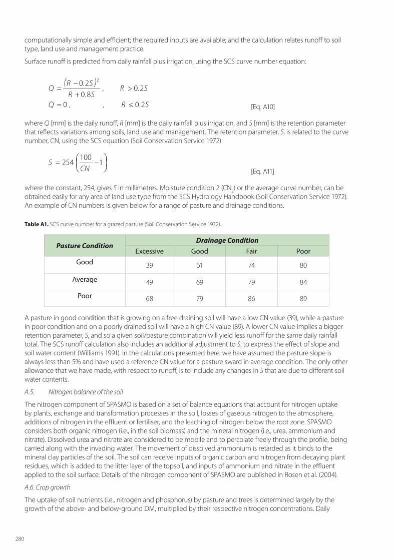
280

computationally simple and efficient; the required inputs are available; and the calculation relates runoff to soil type, land use and management practice.

Surface runoff is predicted from daily rainfall plus irrigation, using the SCS curve number equation:

( )

SRQ

SRSR

SRQ

2.0,,0

2.0,8.0

2.0 2

≤=

>+

−=

[Eq. A10]

where Q [mm] is the daily runoff, R [mm] is the daily rainfall plus irrigation, and S [mm] is the retention parameter that reflects variations among soils, land use and management. The retention parameter, S, is related to the curve number, CN, using the SCS equation (Soil Conservation Service 1972)

−= 1

100254

CNS

[Eq. A11]

where the constant, 254, gives S in millimetres. Moisture condition 2 (CN2) or the average curve number, can be obtained easily for any area of land use type from the SCS Hydrology Handbook (Soil Conservation Service 1972). An example of CN numbers is given below for a range of pasture and drainage conditions.

Table A1. SCS curve number for a grazed pasture (Soil Conservation Service 1972).

Pasture ConditionDrainage Condition

Excessive Good Fair PoorGood 39 61 74 80

Average 49 69 79 84

Poor 68 79 86 89

A pasture in good condition that is growing on a free draining soil will have a low CN value (39), while a pasture in poor condition and on a poorly drained soil will have a high CN value (89). A lower CN value implies a bigger retention parameter, S, and so a given soil/pasture combination will yield less runoff for the same daily rainfall total. The SCS runoff calculation also includes an additional adjustment to S, to express the effect of slope and soil water content (Williams 1991). In the calculations presented here, we have assumed the pasture slope is always less than 5% and have used a reference CN value for a pasture sward in average condition. The only other allowance that we have made, with respect to runoff, is to include any changes in S that are due to different soil water contents.

A.5. Nitrogen balance of the soil

The nitrogen component of SPASMO is based on a set of balance equations that account for nitrogen uptake by plants, exchange and transformation processes in the soil, losses of gaseous nitrogen to the atmosphere, additions of nitrogen in the effluent or fertiliser, and the leaching of nitrogen below the root zone. SPASMO considers both organic nitrogen (i.e., in the soil biomass) and the mineral nitrogen (i.e., urea, ammonium and nitrate). Dissolved urea and nitrate are considered to be mobile and to percolate freely through the profile, being carried along with the invading water. The movement of dissolved ammonium is retarded as it binds to the mineral clay particles of the soil. The soil can receive inputs of organic carbon and nitrogen from decaying plant residues, which is added to the litter layer of the topsoil, and inputs of ammonium and nitrate in the effluent applied to the soil surface. Details of the nitrogen component of SPASMO are published in Rosen et al. (2004).

A.6. Crop growth

The uptake of soil nutrients (i.e., nitrogen and phosphorus) by pasture and trees is determined largely by the growth of the above- and below-ground DM, multiplied by their respective nitrogen concentrations. Daily

281

biomass production is modelled using a potential production rate per unit ground area, G (kg m-2 d-1) that is related, via a conversion efficiency, ε (kg MJ-1), to the amount of solar radiant energy, Φ (MJ m-2 d-1), intercepted by the leaves

WNT fffG Φ= ε [Eq. A12]

Here fT, fN and fW are response functions that range between zero and unity depending on temperature, plant nitrogen and soil water status respectively (Eckersten & Jansson 1991). The value of G depends on the daily sunshine and temperature, plus the leaf-area index of the crop, and is moderated by the soil’s water and nitrogen status (King 2003). Crop growth is maximised only if soil water and soil nutrients are non-limiting.

A simple allometric relationship is used to partition the daily biomass production into the growth of the foliage, stem material and roots. Plant biomass is expressed in terms of the balance between growth and senescence of the plant organs. For each plant organ we write out a simple mass balance equation that considers inputs of DM due to carbon allocation, losses of DM as the plants senescence, and the removal of DM as the plants are harvested. The total mass of foliage, F [kg m-2] is calculated from

FFF HFGdt

dF−−= γα

[Eq. A13]

the total mass of stem material, S [kg m-2] is calculated from

SSS HFGdtdS

−−= γα [Eq. A14]

and the total mass of roots, R [kg m-2], is calculated from

RGdtdR

RR γα −= [Eq. A15]

Here αF is the fraction of biomass partitioned to the foliage, αS is the biomass partitioned to the stem, and αR (=1-αF-αS) is the fraction of biomass allocated to the roots, and γ is the corresponding senescence rate for these plant components. The variable H is used to represent the amount of DM that is removed during harvest. In the case of fruiting crops, additional terms are included in each balance equation to represent an amount of DM transferred to fruit production.

Allocation of DM to the roots depends on the leaf nitrogen content [N]F, having a minimum value [αR0] at a maximum leaf concentration [N]Fx, and increasing as NL decreases (Eckersten & Jansson 1991)

( )( )( ) 5.020 ][/][][11 FxFFxRR NNN −−−+= αα [Eq. A16]

This formulation enables SPASMO to accommodate seasonal changes in DM allocation associated with a changing leaf nutrient status. For simplicity, any seasonal changes in senescence rates have been neglected in the model because we are concerned with the long-term consequences of DM allocation.

A.7. Nitrogen and phosphorus uptake

The model assumes plant growth will achieve a maximum potential only if water, nitrogen and phosphorus are non-limiting. The nitrogen demand for crop growth is set by the maximum nitrogen content of the root [N]Rx, leaf [N]Fx and stem [N]Sx material. During active growth the plant tries to supply new DM material with nitrogen corresponding to these maximum concentrations. The potential uptake of nitrogen, UN [kg ha-1 d-1], is defined as

( )( ) ( )RRRRxRSSSSxS

FFFFxFN

NRNGNSNG

NFNGU

][][][][

][][

γλαγλαγλα

−+−+

−= [Eq. A17]

282

And this represents the new growth at the maximum N content minus an amount of nitrogen translocated from the senescing plant material. The potential (maximum) nitrogen uptake can only be met if sufficient nitrogen exists in the soil. Otherwise all [N]s will be reduced in low-nitrogen soils, and crop growth will be curtailed. The potential uptake of phosphorus uptake is modelled in the same way based on the maximum P content of the respective plant parts.

Daily uptake of nitrogen is assumed to be proportional to the local distribution of the fine roots, and the total amount of nitrate (NO3

-) and ammonium (NH4+) in each soil layer (Johnsson et al. 1987). The potential uptake of

nitrate is calculated as

+= −

+−

−

− 343

33 ,)(min NOfU

NHNONO

zU MNRNO ρ

[Eq. A18]

based on the relative root fraction in the layer, ρR(z), the proportion of total mineral nitrogen as nitrate, and the total growth requirement for nitrogen, UN. However, the actual uptake of nitrate is limited to a fraction fM [-] of the total nitrate available in each layer. Ammonium uptake is calculated in a similar way, being proportional to the relative amount of ammonium in solution.

Surface roots are the most active (Clothier & Green 1994) and they preferentially extract soil water and nutrients from the upper soil layers. However, as water and nitrogen stresses develop, the uptake activity typically switches to the deeper roots if more water and nutrients are available there. This feature of root action is modelled in the following way. Whenever the total nitrogen uptake from a given soil layer is less than the potential rate, then the model allows for a compensatory increase in uptake from remaining layers deeper in the root zone (Johnnson et al. 1987). This is achieved by adding a fraction cum [-] of the deficit to the potential uptake from the next soil layer where more mineral nitrogen may be available.

Daily allocation of nitrogen to the new plant material is based on the idea that roots receive nitrogen first, until they reach their maximum concentrations, then nitrogen is allocated to the stem, and finally to the leaves. If soil nitrogen becomes limiting, a reduction factor fN is used to reduce the total nitrogen uptake. This reduction function also effectively reduces the leaf nitrogen contents and alters the DM allocation pattern (Eckersten & Jansson 1991). A similar scheme is adopted for P uptake and allocation across the new plant material.

Pasture growth parameters in this study have been chosen to generate appropriate levels of DM production i.e. the model simulates between 10–15 T DM ha-1 yields from an irrigated pasture, and adds about 1000 kg DM for every 100 kg N ha-1 of nitrogen in the effluent.

A.8. Carbon and nitrogen dynamics of the soil organic matter

The decomposition of soil biomass adds an amount of mineral nitrogen, in the form of ammonium, to the soil. This transformation process, known as mineralization, is modelled by dividing the soil’s total organic matter into three pools – a fast cycling litter pool, an almost stable humus pool, and a manure pool (Johnsson et al. 1987). The relative amount of organic N in these three pools changes daily to reflect inputs of fresh biomass, and manure, and the losses of soil biomass and plant residue as it decomposes. The nitrogen demand for this internal cycling of the soil’s organic carbon and nitrogen is regulated by the C/N ratio of the soil biomass, rO, which is one of the model inputs.

Decomposition of soil litter carbon (CL) is modelled as a first-order process and is specified by a rate constant (KL) that is influenced by temperature and soil moisture. The products of decomposition are CO2, stabilized organic material (humus) and, conceptually, microbial biomass and metabolites. The relative amount of these products is determined by a synthesis efficiency constant (fE) and a humification fraction (fH). The following mass balance equations, which represent the inputs minus the outputs of soil-C and soil-N, are used to model the turnover of carbon and nitrogen in the litter pool

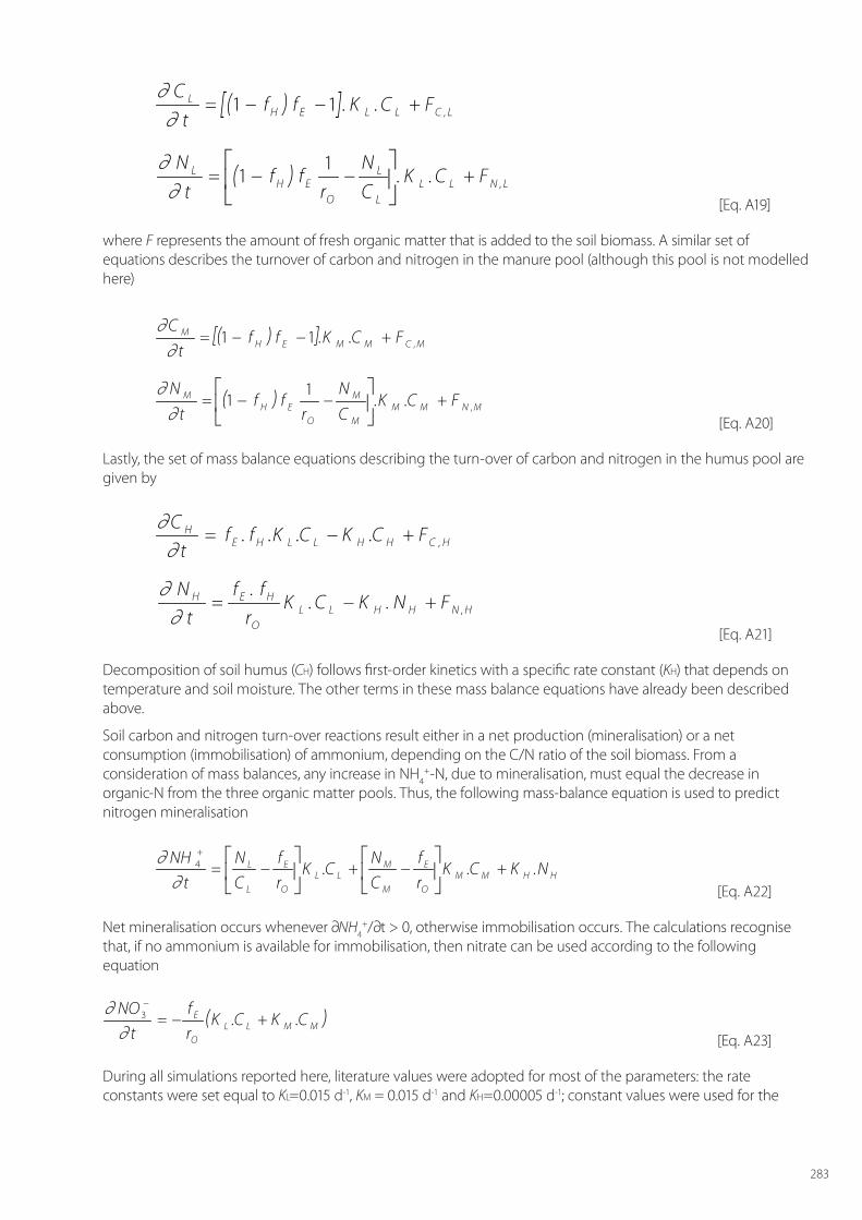
283

( )[ ]∂∂

Ct

f f K C FLH E L L C L= − − +1 1 . . ,

( )∂∂

Nt

f fr

NC

K C FLH E

O

L

LL L N L= − −

+1

1. . ,

[Eq. A19]

where F represents the amount of fresh organic matter that is added to the soil biomass. A similar set of equations describes the turnover of carbon and nitrogen in the manure pool (although this pool is not modelled here)

( )[ ] MCMMEHM FCKfft

C,..11 +−−=

∂∂

( ) MNMMM

M

OEH

M FCKCN

rff

tN

,..1

1 +

−−=

∂∂

[Eq. A20]

Lastly, the set of mass balance equations describing the turn-over of carbon and nitrogen in the humus pool are given by

HCHHLLHEH FCKCKff

tC

,.... +−=∂

∂

∂∂N

tf f

rK C K N FH E H

OL L H H N H= − +

.. . ,

[Eq. A21]

Decomposition of soil humus (CH) follows first-order kinetics with a specific rate constant (KH) that depends on temperature and soil moisture. The other terms in these mass balance equations have already been described above.

Soil carbon and nitrogen turn-over reactions result either in a net production (mineralisation) or a net consumption (immobilisation) of ammonium, depending on the C/N ratio of the soil biomass. From a consideration of mass balances, any increase in NH4

+-N, due to mineralisation, must equal the decrease in organic-N from the three organic matter pools. Thus, the following mass-balance equation is used to predict nitrogen mineralisation

HHMMO

E

M

MLL

O

E

L

L NKCKrf

CN

CKrf

CN

tNH

...4 +

−+

−=

+

∂∂

[Eq. A22]

Net mineralisation occurs whenever ∂NH4+/∂t > 0, otherwise immobilisation occurs. The calculations recognise

that, if no ammonium is available for immobilisation, then nitrate can be used according to the following equation

( )MMLLO

E CKCKrf

tNO

..3 +−=−

∂∂

[Eq. A23]

During all simulations reported here, literature values were adopted for most of the parameters: the rate constants were set equal to KL=0.015 d-1, KM = 0.015 d-1 and KH=0.00005 d-1; constant values were used for the

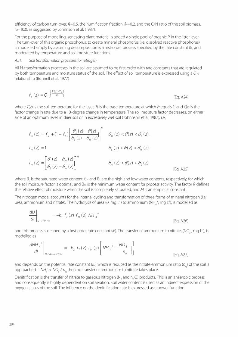
284

efficiency of carbon turn-over, fE=0.5, the humification fraction, fH=0.2, and the C/N ratio of the soil biomass, rO=10.0, as suggested by Johnnson et al. (1987).

For the purpose of modelling, senescing plant material is added a single pool of organic P in the litter layer. The turn-over of this organic phosphorus, to create mineral phosphorus (i.e. dissolved reactive phosphorus) is modelled simply by assuming decomposition is a first-order process specified by the rate constant KL, and moderated by temperature and soil moisture functions.

A.11. Soil transformation processes for nitrogen

All N-transformation processes in the soil are assumed to be first-order with rate constants that are regulated by both temperature and moisture status of the soil. The effect of soil temperature is expressed using a Q10 relationship (Bunnell et al. 1977)

−

= 10)(

10)(BTzT

T Qzf [Eq. A24]

where T(z) is the soil temperature for the layer, TB is the base temperature at which fT equals 1, and Q10 is the factor change in rate due to a 10-degree change in temperature. The soil moisture factor decreases, on either side of an optimum level, in drier soil or in excessively wet soil (Johnnson et al. 1987), i.e.,

),()()()()(

)()()1()( zzz

zzzz

ffzf SH

M

HS

SSSW θθθ

θθθθ

<<

−−

−+=

),()()(1)( zzzzf HLW θθθ <<=

),()()()()(

)()()( zzz

zz

zzzf LW

M

WL

WW θθθ

θθ

θθ<<

−

−=

[Eq. A25]

where θS is the saturated water content, θH and θL are the high and low water contents, respectively, for which the soil moisture factor is optimal, and θW is the minimum water content for process activity. The factor fS defines the relative effect of moisture when the soil is completely saturated, and M is an empirical constant.

The nitrogen model accounts for the internal cycling and transformation of three forms of mineral nitrogen (i.e. urea, ammonium and nitrate). The hydrolysis of urea (U, mg L-1) to ammonium (NH4

+, mg L-1), is modelled as

+

+→

−= 414

)()( NHzfzfkdt

dUMT

NHU

[Eq. A26]

and this process is defined by a first-order rate constant (k1). The transfer of ammonium to nitrate, (NO3-, mg L-1), is

modelled as

−−−= +

−→+

+

qMT

NNHn

NONHzfzfk

dtdNH 3

42

034

4 )()(

[Eq. A27]

and depends on the potential rate constant (k2) which is reduced as the nitrate-ammonium ratio (nq) of the soil is approached. If NH4

+ < NO3 -/ nq then no transfer of ammonium to nitrate takes place.

Denitrification is the transfer of nitrate to gaseous nitrogen (N2 and N2O) products. This is an anaerobic process and consequently is highly dependent on soil aeration. Soil water content is used as an indirect expression of the oxygen status of the soil. The influence on the denitrification rate is expressed as a power function

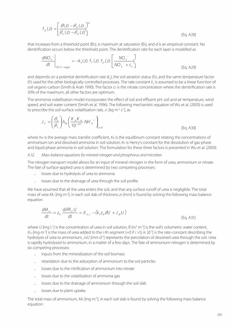
285

d

DS

DD zz

zzzf

−

−=

)()()()(

)(θθ

θθ [Eq. A28]

that increases from a threshold point (θD), is maximum at saturation (θS), and d is an empirical constant. No denitrification occurs below the threshold point. The denitrification rate for each layer is modelled as

+−= −

−

→−

−

SDT

gasNOcNO

NOzfzfzk

dtdNO

3

33

3

3 )()()(

[Eq. A29]

and depends on a potential denitrification rate (k3), the soil aeration status (fD), and the same temperature factor (fT) used for the other biologically-controlled processes. The rate constant k3 is assumed to be a linear function of soil organic-carbon (Smith & Arah 1990). The factor cS is the nitrate concentration where the denitrification rate is 50% of the maximum, all other factors are optimum.

The ammonia volatilisation model incorporates the effect of soil and effluent pH, soil and air temperature, wind speed, and soil water content (Smith et al. 1996). The following mechanistic equation of Wu et al. (2003) is used to prescribe the soil-surface volatilisation rate, JV [kg m-2 s-1], as

04

0

10 =

+−

=

zpH

HAM

SV NH

KKhJ

θθ

[Eq. A30]

where hM is the average mass transfer coefficient, KA is the equilibrium constant relating the concentrations of ammonium ion and dissolved ammonia in soil solution, KH is Henry’s constant for the dissolution of gas-phase and liquid-phase ammonia in soil solution. The formulation for these three factors is presented in Wu et al. (2003).

A.12. Mass-balance equations for mineral nitrogen and phosphorus and microbes

The nitrogen transport model allows for an input of mineral nitrogen in the form of urea, ammonium or nitrate. The fate of surface-applied urea is determined by two competing processes:

. losses due to hydrolysis of urea to ammonia

. losses due to the drainage of urea through the soil profile.

We have assumed that all the urea enters the soil, and that any surface runoff of urea is negligible. The total mass of urea MU [mg m-2], in each soil slab of thickness zR [mm] is found by solving the following mass balance equation

( )UJUzkXdt

URdz

dtdM

WRiUU

RU +−== θ

θ1,

[Eq. A31]

where U [mg L-1] is the concentration of urea in soil solution, θ [m3 m-3] is the soil’s volumetric water content, XU,i [mg m-2] is the mass of urea added to the i-th segment (=0 if i >1), k1 [d-1] is the rate-constant describing the hydrolysis of urea to ammonium, JWU [mm d-1] represents the percolation of dissolved urea through the soil. Urea is rapidly hydrolysed to ammonium, in a matter of a few days. The fate of ammonium-nitrogen is determined by six competing processes:

. inputs from the mineralization of the soil biomass

. retardation due to the adsorption of ammonium to the soil particles

. losses due to the nitrification of ammonium into nitrate

. losses due to the volatilization of ammonia gas

. losses due to the drainage of ammonium through the soil slab

. losses due to plant uptake.

The total mass of ammonium, MA [mg m-2], in each soil slab is found by solving the following mass balance equation:

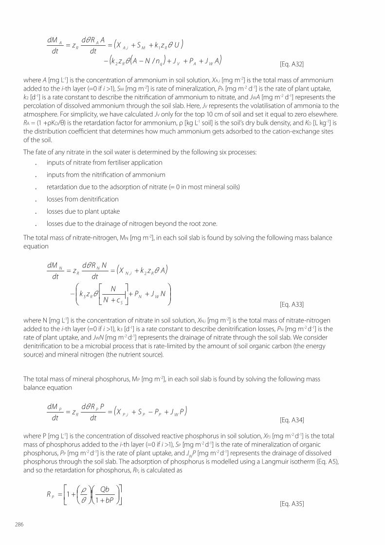
286

( )( )( )AJPJnNAzk

UzkSXdt

ARdz

dtdM

WAVqR

RMiAA

RA

+++−−

++==

/2

1,

θ

θθ

[Eq. A32]

where A [mg L-1] is the concentration of ammonium in soil solution, XA,i [mg m-2] is the total mass of ammonium added to the i-th layer (=0 if i >1), SM [mg m-2] is rate of mineralization, PA [mg m-2 d-1] is the rate of plant uptake, k2 [d-1] is a rate constant to describe the nitrification of ammonium to nitrate, and JWA [mg m-2 d-1] represents the percolation of dissolved ammonium through the soil slab. Here, JV represents the volatilisation of ammonia to the atmosphere. For simplicity, we have calculated JV only for the top 10 cm of soil and set it equal to zero elsewhere. RA = (1 +ρKD/θ) is the retardation factor for ammonium, ρ [kg L-1 soil] is the soil’s dry bulk density, and KD [L kg-1] is the distribution coefficient that determines how much ammonium gets adsorbed to the cation-exchange sites of the soil.

The fate of any nitrate in the soil water is determined by the following six processes: . inputs of nitrate from fertiliser application

. inputs from the nitrification of ammonium

. retardation due to the adsorption of nitrate (= 0 in most mineral soils)

. losses from denitrification

. losses due to plant uptake

. losses due to the drainage of nitrogen beyond the root zone.

The total mass of nitrate-nitrogen, MN [mg m-2], in each soil slab is found by solving the following mass balance equation

( )

++

+

−

+==

NJPcN

Nzk

AzkXdt

NRdz

dtdM

WNS

R

RiNN

RN

θ

θθ

3

2,

[Eq. A33]

where N [mg L-1] is the concentration of nitrate in soil solution, XN,i [mg m-2] is the total mass of nitrate-nitrogen added to the i-th layer (=0 if i >1), k3 [d-1] is a rate constant to describe denitrification losses, PN [mg m-2 d-1] is the rate of plant uptake, and JWN [mg m-2 d-1] represents the drainage of nitrate through the soil slab. We consider denitrification to be a microbial process that is rate-limited by the amount of soil organic carbon (the energy source) and mineral nitrogen (the nutrient source).

The total mass of mineral phosphorus, MP [mg m-2], in each soil slab is found by solving the following mass balance equation

( )PJPSXdt

PRdz

dtdM

WPPiPP

RP +−+== ,

θ

[Eq. A34]

where P [mg L-1] is the concentration of dissolved reactive phosphorus in soil solution, XP,i [mg m-2 d-1] is the total mass of phosphorus added to the i-th layer (=0 if i >1), SP [mg m-2 d-1] is the rate of mineralization of organic phosphorus, PP [mg m-2 d-1] is the rate of plant uptake, and JWP [mg m-2 d-1] represents the drainage of dissolved phosphorus through the soil slab. The adsorption of phosphorus is modelled using a Langmuir isotherm (Eq. A5), and so the retardation for phosphorus, RP, is calculated as

+

+=

bPQb

R P 11

θρ

[Eq. A35]

287

where Q is the maximum total mass of phosphorus at saturation per unit mass of dry soil [µg g-1], and b is an empirical constant, with units of inverse of solution concentration [L mg-1].

Bacterial transport is calculated using the same convection-dispersion type equation for water and solute transport, with additional terms used to represent the kinetic sorption of bacteria to the soil’s mineral particles as well as the subsequent detachment and transfer of bacteria between the aqueous and solid phases (Schijven & Hassanizadeh 2000). The mass balance equation for water-borne bacteria (considering only those bacteria applied in the effluent) is given by the following equation

( )BJSBSkBkXdt

BdWSWdaiB −−−+−= ρµθµρψθ

θ,

[Eq. A36]

where B represents the bacteria concentration in the liquid phase [cfu L-1], SB represents the bacteria concentration in the solid (sorbed) phase [cfu g-1], XB,i is the total mass of bacteria added to the i-th layer (=0 if i >1) [cfu m-2 d-1], the ka term represents attachment of bacteria to the soil particles, and the kd term represents detachment of bacteria from the soil particles and JWB [mg m-2 d-1] represents the drainage of bacteria through the soil slab. The inactivation (die-off) of bacteria is described using a simple first-order decay model, where μ is the mortality rate [d-1] and the subscripts ‘w’ and ‘s’ refer to the liquid and solid phases, respectively. The overall mortality rate for E. coli bacteria in soil has been reported to be between 0.09 and 0.17 d-1 in two contrasting silt loams (Mubiru et al. 2000). Sukias & Nguyen (2003) report the rate constant for bacterial die-off in a Te Kowai silt loam, from Hamilton, is about 0.056 d-1. This represents a ‘half-life’ of between about 1.8 and 3.3 days.

Calculation procedure

The model is run using a daily time step, to track the fate of nutrients and contaminants in effluent-applied land. The model considers the 11 irrigation areas separately, adding different amount of effluent to each site depending on pond disposal requirements and set irrigation rules. The calculations are made in the following sequence:

. subtract evaporation, transpiration and plant uptake of nutrients from each soil segment

. add and subtract the nitrogen, phosphorus and bacteria involved in the various transformation processes

. partition each contaminant between solution and sorbed fractions, assuming complete equilibrium between the mobile and immobile phases

. if there is rain or irrigation, then perform the leaching process

. redistribute water and contaminants vertically, according to water potential and solution concentration

. repeat the contaminant partitioning.

288

A.13 Appendix ReferencesAllen, R.G.; Pereira, L.S.; Raes, D.; Smith, M. (1998). Crop Evapotranspiration. Guidelines for computing crop water requirements. FAO Irrigation and Drainage Paper No. 56. Food and Agriculture Organization of the United Nations, Rome, 301 p.

Bunnell, F.L.; Tait, D.E.N.; Flanagan, P.W.; Van Cleve, K. (1977). Microbial respiration and substrate weight loss. Soil Biology and Biochemistry 9: 33-40.

Clothier, B.E.; Green, S.R. (1994). Rootzone processes and the efficient use of irrigation water. Agricultural Water Management 25: 1-12.

Eckersten, H.; Jansson, P.E. (1991). Modelling water flow, nitrogen uptake and production for wheat. Fertilizer Research 27: 313-330.

Green S.R.; Vogeler, I.; Clothier, B.E.; Mills, T.M.; van den Dijssel, C. (2002). Modelling water uptake by a mature apple tree. Australian Journal of Soil Research 41: 365-380.

Green, S.R.; McNaughton, K.G.; Wunsche, J.N.; Clothier, B.E. (2003). Modelling light interception and transpiration of apple trees. Agronomy Journal 95: 1380-1387.

Hutson, J.L.; Wagenet, R.J. (1993). A pragmatic field-scale approach for modeling pesticides. Journal of Environmental Quality 22: 494 – 499.

Johnnson, H.; Bergstrom, L.; Jannson, P.E.; Paustian, K. (1987). Simulated nitrogen dynamics and losses in a layered agricultural soil. Agriculture Ecosystems and Environment 18: 333-356.

Johnson, P.R.; Elimelech, M. (1995). Dynamics of colloid deposition in porous media: Blocking based on random sequential adsorption. Langmuir 11: 801-812.

King, D.A. (2003). Allocation of above-ground growth is related to light in temperate deciduous saplings. Functional Ecology 17: 482-488.

Logan, B.E.; Jewett, D.G.; Arnold, R.G.; Bouwer, E.J.; O’Melia, C.R. (1995). Clarification of clean-bed filtration models. Journal of Environmental Engineering 121: 869–873.

Mubiru, D.N.; Coyne, M.S.; Grove, J.H. (2000). Mortality of Escherichia coli O157:H7 in two soils with different physical and chemical properties. Journal Environmental Quality 29: 1821-1825.

Rosen, M.R.; Reeves, R.R.; Green, S.R.; Clothier, B.E.; Ironside, N. (2004). Prediction of groundwater nitrate contamination after closure of an unlined sheep feed lot in New Zealand. Vadose Journal 3: 990-1006.

Schijven, J.F.; Hassanizadeh, S.M. (2000). Removal of viruses by soil passage: Overview of modelling, processes and parameters. Critical Reviews in Environmental Science and Technology 30: 49-127.

Simunek, J.; van Genuchten, M.T.; Sejna, M. (2005). The HYDRUS-1D Software package for simulating the one-dimensional movement of water, heat and multiple solutes in variably saturated media.

Smith, K.A.; Arah, J.R.M. (1990). Losses of nitrogen by denitrification and emissions of nitrogen oxides from soils. Proceedings of Fertiliser Society 299: 1-34.

Smith, C.J.; Freney, J.R.; Bond, W.J. (1996). Ammonia volatilization from soil irrigated with urban sewerage effluent. Australian Journal of Soil Researcg 34: 789-802.

Soil Conservation Service (1972). Hydrology. ‘SCS National Engineering Handbook.’ Section 4. U.S. Govt Printing Office: Washington D.C.

Sukias, J.P.S.; Nguyen, M.L. (2003). Inactivation of E. coli in riparian and non-riparian soils. Diffuse pollution 7th International Specialized Conference on Diffuse Pollution and Basin Management, Dublin, Ireland, August 18-22, 2003, pp 3.82-3.87.

Williams, J.R. (1991). Runoff and water erosion. In Hanks, J.; Ritchie. J.T. (Eds.), Modelling plant and soil systems. Agonomy No. 31 series, American Society of Agronomy, Madison, USA.

Wu, J.; Nofziger, D.L.; Warren, J.G; Hattey, J.A. (2003). Modelling ammonia volatilization from surface-applied swine effluent. Soil Science Society Journal of America 67: 1-11.

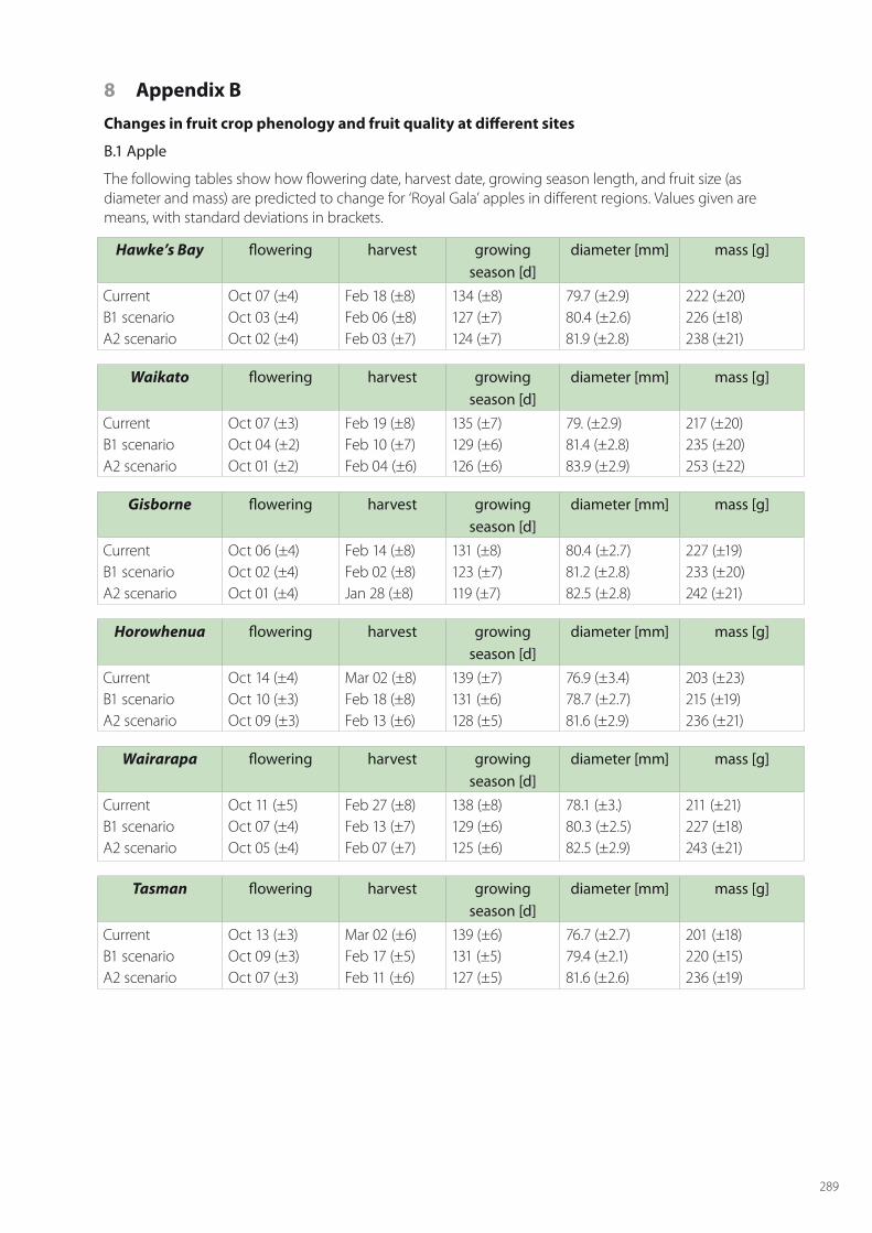
289

8 Appendix B

Changes in fruit crop phenology and fruit quality at different sites

B.1 Apple

The following tables show how flowering date, harvest date, growing season length, and fruit size (as diameter and mass) are predicted to change for ‘Royal Gala’ apples in different regions. Values given are means, with standard deviations in brackets.

Hawke’s Bay flowering harvest growing season [d]

diameter [mm] mass [g]

CurrentB1 scenarioA2 scenario

Oct 07 (±4)Oct 03 (±4)Oct 02 (±4)

Feb 18 (±8)Feb 06 (±8)Feb 03 (±7)

134 (±8)127 (±7)124 (±7)

79.7 (±2.9)80.4 (±2.6)81.9 (±2.8)

222 (±20)226 (±18)238 (±21)

Waikato flowering harvest growing season [d]

diameter [mm] mass [g]

CurrentB1 scenarioA2 scenario

Oct 07 (±3)Oct 04 (±2)Oct 01 (±2)

Feb 19 (±8)Feb 10 (±7)Feb 04 (±6)

135 (±7)129 (±6)126 (±6)

79. (±2.9)81.4 (±2.8)83.9 (±2.9)

217 (±20)235 (±20)253 (±22)

Gisborne flowering harvest growing season [d]

diameter [mm] mass [g]

CurrentB1 scenarioA2 scenario

Oct 06 (±4)Oct 02 (±4)Oct 01 (±4)

Feb 14 (±8)Feb 02 (±8)Jan 28 (±8)

131 (±8)123 (±7)119 (±7)

80.4 (±2.7)81.2 (±2.8)82.5 (±2.8)

227 (±19)233 (±20)242 (±21)

Horowhenua flowering harvest growing season [d]

diameter [mm] mass [g]

CurrentB1 scenarioA2 scenario

Oct 14 (±4)Oct 10 (±3)Oct 09 (±3)

Mar 02 (±8)Feb 18 (±8)Feb 13 (±6)

139 (±7)131 (±6)128 (±5)

76.9 (±3.4)78.7 (±2.7)81.6 (±2.9)

203 (±23)215 (±19)236 (±21)

Wairarapa flowering harvest growing season [d]

diameter [mm] mass [g]

CurrentB1 scenarioA2 scenario

Oct 11 (±5)Oct 07 (±4)Oct 05 (±4)

Feb 27 (±8)Feb 13 (±7)Feb 07 (±7)

138 (±8)129 (±6)125 (±6)

78.1 (±3.)80.3 (±2.5)82.5 (±2.9)

211 (±21)227 (±18)243 (±21)

Tasman flowering harvest growing season [d]

diameter [mm] mass [g]

CurrentB1 scenarioA2 scenario

Oct 13 (±3)Oct 09 (±3)Oct 07 (±3)

Mar 02 (±6)Feb 17 (±5)Feb 11 (±6)

139 (±6)131 (±5)127 (±5)

76.7 (±2.7)79.4 (±2.1)81.6 (±2.6)

201 (±18)220 (±15)236 (±19)

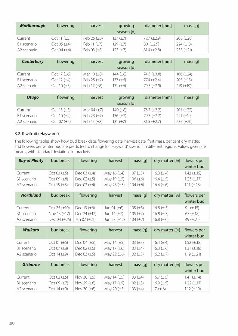
290

Marlborough flowering harvest growing season [d]

diameter [mm] mass [g]

CurrentB1 scenarioA2 scenario

Oct 11 (±5)Oct 05 (±4)Oct 04 (±4)

Feb 25 (±8)Feb 11 (±7)Feb 03 (±8)

137 (±7)129 (±7)123 (±7)

77.7 (±2.9)80. (±2.5)81.4 (±2.8)

208 (±20)224 (±18)235 (±21)

Canterbury flowering harvest growing season [d]

diameter [mm] mass [g]

CurrentB1 scenarioA2 scenario

Oct 17 (±6)Oct 12 (±4)Oct 10 (±5)

Mar 10 (±8)Feb 25 (±7)Feb 17 (±8)

144 (±8)137 (±6)131 (±6)

74.5 (±3.8)77.4 (±2.4)79.3 (±2.9)

186 (±24)205 (±15)219 (±19)

Otago flowering harvest growing season [d]

diameter [mm] mass [g]

CurrentB1 scenarioA2 scenario

Oct 15 (±5)Oct 10 (±4)Oct 07 (±5)

Mar 04 (±7)Feb 23 (±7)Feb 15 (±8)

140 (±8)136 (±7)131 (±7)

76.7 (±3.2)79.5 (±2.7)81.5 (±2.7)

201 (±22)221 (±19)235 (±20)

B.2 Kiwifruit (‘Hayward’)

The following tables show how bud break date, flowering date, harvest date, fruit mass, per cent dry matter, and flowers per winter bud are predicted to change for ‘Hayward’ kiwifruit in different regions. Values given are means, with standard deviations in brackets.

Bay of Plenty bud break flowering harvest mass [g] dry matter [%] flowers perwinter bud

CurrentB1 scenarioA2 scenario

Oct 03 (±5)Oct 09 (±8)Oct 15 (±8)

Dec 03 (±4)Dec 02 (±5)Dec 03 (±4)

May 16 (±4)May 19 (±5)May 23 (±5)

107 (±5)106 (±6)104 (±6)

16.3 (±.4)16.4 (±.5)16.4 (±.6)

1.42 (±.15)1.23 (±.17)1.11 (±.18)

Northland bud break flowering harvest mass [g] dry matter [%] flowers perwinter bud

CurrentB1 scenarioA2 scenario

Oct 25 (±10)Nov 13 (±17)Dec 04 (±25)

Dec 13 (±6)Dec 24 (±12)Jan 07 (±21)

Jun 01 (±6)Jun 14 (±7)Jun 27 (±12)

105 (±5)105 (±7)104 (±7)

16.8 (±.5)16.8 (±.7)16.8 (±.6)

.91 (±.15)

.67 (±.18)

.49 (±.21)

Waikato bud break flowering harvest mass [g] dry matter [%] flowers perwinter bud

CurrentB1 scenarioA2 scenario

Oct 01 (±5)Oct 07 (±8)Oct 14 (±9)

Dec 04 (±5)Dec 02 (±6)Dec 03 (±5)

May 14 (±5)May 17 (±6)May 22 (±6)

103 (±3)103 (±4)102 (±3)

16.4 (±.4)16.3 (±.6)16.2 (±.7)

1.52 (±.18)1.31 (±.18)1.19 (±.21)

Gisborne bud break flowering harvest mass [g] dry matter [%] flowers perwinter bud

CurrentB1 scenarioA2 scenario

Oct 02 (±5)Oct 09 (±7)Oct 14 (±9)

Nov 30 (±5)Nov 29 (±6)Nov 30 (±6)

May 14 (±5)May 17 (±5)May 20 (±5)

103 (±4)102 (±3)103 (±4)

16.7 (±.5)16.9 (±.5)17. (±.6)

1.41 (±.14)1.22 (±.17)1.12 (±.19)

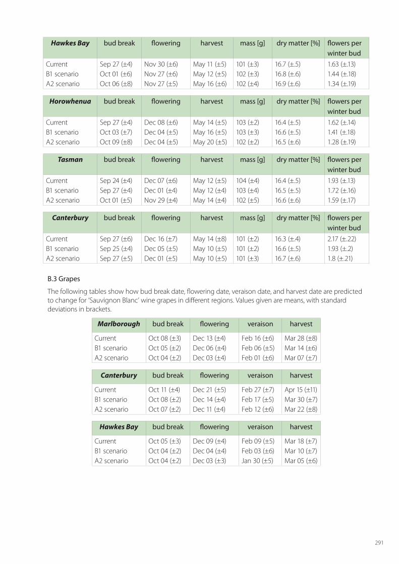
291

Hawkes Bay bud break flowering harvest mass [g] dry matter [%] flowers perwinter bud

CurrentB1 scenarioA2 scenario

Sep 27 (±4)Oct 01 (±6)Oct 06 (±8)

Nov 30 (±6)Nov 27 (±6)Nov 27 (±5)

May 11 (±5)May 12 (±5)May 16 (±6)

101 (±3)102 (±3)102 (±4)

16.7 (±.5)16.8 (±.6)16.9 (±.6)

1.63 (±.13)1.44 (±.18)1.34 (±.19)

Horowhenua bud break flowering harvest mass [g] dry matter [%] flowers perwinter bud

CurrentB1 scenarioA2 scenario

Sep 27 (±4)Oct 03 (±7)Oct 09 (±8)

Dec 08 (±6)Dec 04 (±5)Dec 04 (±5)

May 14 (±5)May 16 (±5)May 20 (±5)

103 (±2)103 (±3)102 (±2)

16.4 (±.5)16.6 (±.5)16.5 (±.6)

1.62 (±.14)1.41 (±.18)1.28 (±.19)

Tasman bud break flowering harvest mass [g] dry matter [%] flowers perwinter bud

CurrentB1 scenarioA2 scenario

Sep 24 (±4)Sep 27 (±4)Oct 01 (±5)

Dec 07 (±6)Dec 01 (±4)Nov 29 (±4)

May 12 (±5)May 12 (±4)May 14 (±4)

104 (±4)103 (±4)102 (±5)

16.4 (±.5)16.5 (±.5)16.6 (±.6)

1.93 (±.13)1.72 (±.16)1.59 (±.17)

Canterbury bud break flowering harvest mass [g] dry matter [%] flowers perwinter bud

CurrentB1 scenarioA2 scenario

Sep 27 (±6)Sep 25 (±4)Sep 27 (±5)

Dec 16 (±7)Dec 05 (±5)Dec 01 (±5)

May 14 (±8)May 10 (±5)May 10 (±5)

101 (±2)101 (±2)101 (±3)

16.3 (±.4)16.6 (±.5)16.7 (±.6)

2.17 (±.22)1.93 (±.2)1.8 (±.21)

B.3 Grapes

The following tables show how bud break date, flowering date, veraison date, and harvest date are predicted to change for ‘Sauvignon Blanc’ wine grapes in different regions. Values given are means, with standard deviations in brackets.

Marlborough bud break flowering veraison harvest

CurrentB1 scenarioA2 scenario

Oct 08 (±3)Oct 05 (±2)Oct 04 (±2)

Dec 13 (±4)Dec 06 (±4)Dec 03 (±4)

Feb 16 (±6)Feb 06 (±5)Feb 01 (±6)

Mar 28 (±8)Mar 14 (±6)Mar 07 (±7)

Canterbury bud break flowering veraison harvest

CurrentB1 scenarioA2 scenario

Oct 11 (±4)Oct 08 (±2)Oct 07 (±2)

Dec 21 (±5)Dec 14 (±4)Dec 11 (±4)

Feb 27 (±7)Feb 17 (±5)Feb 12 (±6)

Apr 15 (±11)Mar 30 (±7)Mar 22 (±8)

Hawkes Bay bud break flowering veraison harvest

CurrentB1 scenarioA2 scenario

Oct 05 (±3)Oct 04 (±2)Oct 04 (±2)

Dec 09 (±4)Dec 04 (±4)Dec 03 (±3)

Feb 09 (±5)Feb 03 (±6)Jan 30 (±5)

Mar 18 (±7)Mar 10 (±7)Mar 05 (±6)

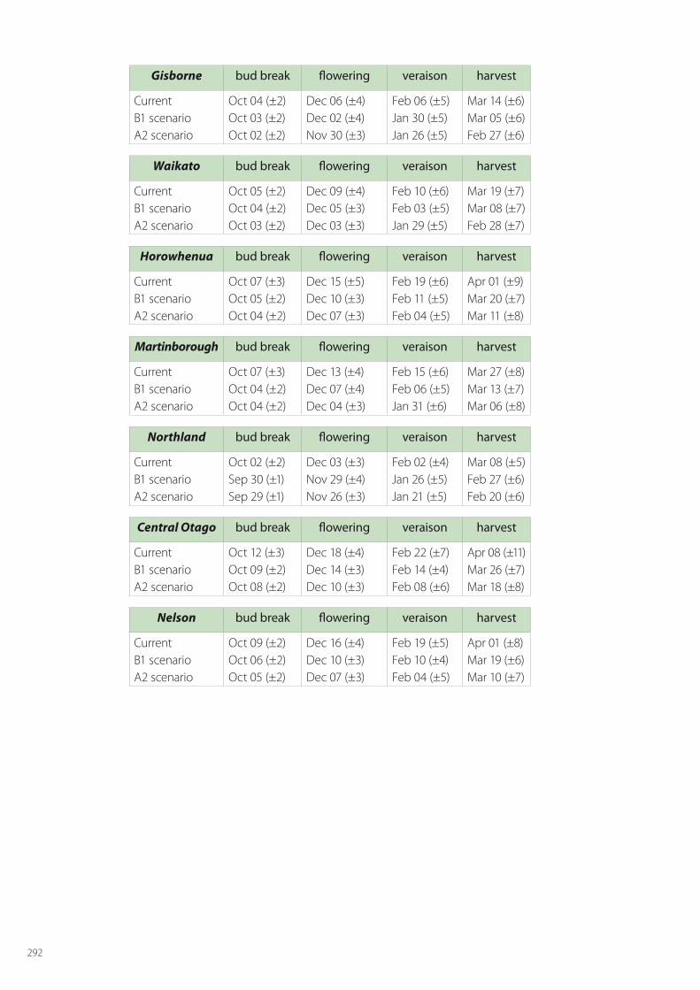
292

Gisborne bud break flowering veraison harvest

CurrentB1 scenarioA2 scenario

Oct 04 (±2)Oct 03 (±2)Oct 02 (±2)

Dec 06 (±4)Dec 02 (±4)Nov 30 (±3)

Feb 06 (±5)Jan 30 (±5)Jan 26 (±5)

Mar 14 (±6)Mar 05 (±6)Feb 27 (±6)

Waikato bud break flowering veraison harvest

CurrentB1 scenarioA2 scenario

Oct 05 (±2)Oct 04 (±2)Oct 03 (±2)

Dec 09 (±4)Dec 05 (±3)Dec 03 (±3)

Feb 10 (±6)Feb 03 (±5)Jan 29 (±5)

Mar 19 (±7)Mar 08 (±7)Feb 28 (±7)

Horowhenua bud break flowering veraison harvest

CurrentB1 scenarioA2 scenario

Oct 07 (±3)Oct 05 (±2)Oct 04 (±2)

Dec 15 (±5)Dec 10 (±3)Dec 07 (±3)

Feb 19 (±6)Feb 11 (±5)Feb 04 (±5)

Apr 01 (±9)Mar 20 (±7)Mar 11 (±8)

Martinborough bud break flowering veraison harvest

CurrentB1 scenarioA2 scenario

Oct 07 (±3)Oct 04 (±2)Oct 04 (±2)

Dec 13 (±4)Dec 07 (±4)Dec 04 (±3)

Feb 15 (±6)Feb 06 (±5)Jan 31 (±6)

Mar 27 (±8)Mar 13 (±7)Mar 06 (±8)

Northland bud break flowering veraison harvest

CurrentB1 scenarioA2 scenario

Oct 02 (±2)Sep 30 (±1)Sep 29 (±1)

Dec 03 (±3)Nov 29 (±4)Nov 26 (±3)

Feb 02 (±4)Jan 26 (±5)Jan 21 (±5)

Mar 08 (±5)Feb 27 (±6)Feb 20 (±6)

Central Otago bud break flowering veraison harvest

CurrentB1 scenarioA2 scenario

Oct 12 (±3)Oct 09 (±2)Oct 08 (±2)

Dec 18 (±4)Dec 14 (±3)Dec 10 (±3)

Feb 22 (±7)Feb 14 (±4)Feb 08 (±6)

Apr 08 (±11)Mar 26 (±7)Mar 18 (±8)

Nelson bud break flowering veraison harvest

CurrentB1 scenarioA2 scenario

Oct 09 (±2)Oct 06 (±2)Oct 05 (±2)

Dec 16 (±4)Dec 10 (±3)Dec 07 (±3)

Feb 19 (±5)Feb 10 (±4)Feb 04 (±5)

Apr 01 (±8)Mar 19 (±6)Mar 10 (±7)

Chapter 7. ForestryLong-term adaptation of productive forests in a changing climatic environment

Andrew Dunningham Scion

Miko Kirschbaum Landcare Research

Tim Payn Scion

Dean Meason Scion