Embed Size (px)
Citation preview

Chapter 6
Finite Element Processing

Chapter 6 Finite Element Processing

Chapter 6 Finite Element Processing 6-1
Finite element analysis consists of several steps from creating geometric coordinate
data to visualizing the analysis results.
The core of the finite element analysis is to form the system equations using the
data pre p a red as described in the previous chapters, and to solve them. This
p ro c e d u re is called “p ro c e s s i n g of finite element analysis,” and termed here as
“finite element processing.” Among all the procedures in finite element analysis,
this is the one which re q u i res minimum user interaction. Once the pro c e s s i n g
begins, it goes on continuously by itself to the end without requiring user
intervention. However, the processing is the step which involves the most
intensive computation. This usually demands huge computational re s o u rces in
terms of computing time and memory space. The computing time for processing
varies largely depending on the size of the problem: from less than a second to
several hours or more. The computing time as well as the memory space required
for finite element processing increases drastically as the size of the pro b l e m
becomes larger, in going from 2-D to 3-D, linear to nonlinear, static to dynamic.
Computational efficiency in terms of computing time and memory space is an
important issue in the finite element processing. There are a number of factors
affecting computational efficiency. Either node numbering or element numbering
depending on the solution scheme is one of the major factors determining the
e ff i c i e n c y. Optimizing the node numbering or the element numbering is an
essential step which should be taken prior to the processing. Accuracy as well as
computational efficiency is affected also by integration schemes and element types
employed in the processing. Therefore, they should be manipulated by the users
for the best accuracy and efficiency.
This chapter describes the usage of functions related with finite element processing
and its computational efficiency. These functions are arranged as items of
menu as shown in the figure below.
Chapter 6 Finite Element Processing
Optimize node numbersOptimize element numbersSet integration schemeChoose analysis output itemsSubmenus for checking node or element connectivityDisplay analysis statusSubmenus for simulation of finite element analysis (CBT)Register external processesLaunch a registered external processTurn on and off auto-solve modeProcess finite element analysis

6-2 Chapter 6 Finite Element Processing
Getting Finite Element Solution
Assembling and solving finite element equations involve many complicated steps
and a huge amount of computation. For you as an end-user, however, it is usually
a simple single step pro c e d u re. All you have to do is to choose an appro p r i a t e
menu item. In spite of this simplicity, it is important for you to understand the
mechanism of this pro c e d u re in order to get a proper solution with maximum
efficiency.
Solver of finite element analysis
T h e re is software specialized in finite element p ro c e s s i n g. They are commonly
called “solver.” VisualFEA has the capability of such as solver embedded in itself.
H o w e v e r, you may use VisualFEA together with other solvers provided by third
p a r t y, or developed by yourself. In other words, you may use VisualFEA for
creating a finite element model (preprocessing) and visualizing the analysis results
( p o s t p rocessing), and use other solvers for processing. Such a finite element
processor is termed here as “external solver.”
T h e re are two paths for doing finite element analysis with VisualFEA: one is
relying only on VisualFEA through the whole procedures, and the other combining
an external solver for processing and VisualFEA for pre- and postprocessing.
<Alternative procedures of FEA using VisualFEA>
The procedure of finite element analysis based only on VisualFEA is simpler, more
s t r a i g h t f o r w a rd and more efficient than that based on the combined usage of
VisualFEA and an external solver. However, the solver embedded in VisualFEA
may not cover the range of problem you want to solve. In such a circ u m s t a n c e ,
Processing PostprocessingPreprocessing
External Solver
Postprocessing
Combined use of VisualFEA and an external solver
Use of intuitiveFEM for whole procedures
Processing
Preprocessing
VisualFEA
VisualFEA

Chapter 6 Finite Element Processing 6-3
you should employ an external solver.
It is your responsibility to make data interface between VisualFEA and external
solvers, unless there exists software interfacing them. The data interface is
described in Chapter 10.
Processing of structural analysis
The simplest method of getting a finite element solution is to use VisualFEA’s own
processing capability. The finite element solver’s capabilities are embedded within
VisualFEA. This makes VisualFEA much simpler to use than other finite element
p rograms which has separate module for processing, pr e p rocessing and
postprocessing.
In order to get into the processing stage for solution, choose “S o l v e” item fro m
menu Then, “Analysis Options” d i a l o g appears on the screen. The
contents of the dialog vary depending on the type of solution as will be described
b e l o w. Set the dialog items as desired and click button. Then, the
p rocessing starts, and goes on up to the completion of all the necessary
computation including assembling the system equations and solving them.
■ Setting analysis options for linear static analysis
Choosing “Solve” item from menu will pop up "Analysis Options" dialog
as shown below, if you have set the solution type as linear static. The solution type
is initially set as linear static, and remains as it is, unless you have checked any one of the
check boxes under "Solution Type", i.e., "Material nonlinear", "Geometric nonlinear" and
"Dynamic."
The dialog has a few items setting the options related to the finite element
solution procedure.
Set the solution stage
Select the equation solver
Set the processing options

6-4 Chapter 6 Finite Element Processing
• solution stage: The solution stage may be set as one of “Analysis,”
“Reanalysis” and "Adaptive." If you turn on "Adaptive" radio button, the
solution pro c e d u re turns into adaptive process. The analysis options for
adaptive analysis are described in the next section. So, only "Analysis" and
"Reanalysis" options are described in this section.
The initial default setting of the solution stage is “Analysis”, which leads to
the normal pro c e d u re of processing based on assembling equations and
solving them. Once the system equations are assembled and solved, they
may be used for subsequent processing by setting the option as “Reanalysis”.
The reanalysis option will eliminate most of the computing time for
assembling and decomposing the system equations. The reanalysis option is
enabled and valid only under the following conditions.
- The system equations should have been solved in the previous session.
- The files containing the system equations should exist in the same directory
(folder) as the data file.
In order to keep these file for reanalysis in next sessions, check “Keep the matrix for
reanalysis” item in the “Analysis Options” dialog.
- G e o m e t r y, element properties, and boundary conditions should not have
been altered since the system equation files were created.
Loads may be changed.
- The analysis type is linear static, and not adaptive nor sequential.
• equation solver: You may choose one of two methods of assembling and
solving equations: frontal method and skyline method. They are typical and
the most widely used methods in finite element analysis solvers.
Skyline method uses only CPU memory, while frontal method relies much on
auxiliary memory such as a hard disk. Accordingly skyline method demands
much larger CPU memory space than frontal method. Skyline method
usually works faster than the frontal method which requires frequent reading
and writing with the auxiliary memory.
The default setting is “Frontal.” If your computer is equipped with huge CPU
m e m o r y, and you want faster solution, choose “Skyline.” Otherwise, you
should keep the option as “Frontal.”
In case you chose “Skyline,” but the memory space is not sufficient, the
software will notify this by the following message box. If you click
button of the dialog, the software will automatically switch the solver to
“Frontal.”

Chapter 6 Finite Element Processing 6-5
• processing options: You can turn on or off each of the processing options by
clicking the check box in front of each item. These settings are applied
during the processing stage.
- “Optimize element number” : This item is enabled only when the equation
solver is set as “Frontal”. If this option is turned on, optimization of element
numbering is automatically done prior to assembling the system equations.
- “O p t i m i z e node number” : This item is enabled only when the equation
solver is set as “Skyline”. If this option is turned on, optimization of node
numbering is automatically done prior to assembling the system equations.
- “Visualize the process” : If this option is turned on, a graphical rendering of
the model is provided along with the status of the element stiffness matrix
assembly.
- “Keep the matrix for re a n a l y s i s” : The system equation files are created at
the start of matrix assemblage and removed at the end of the processing. In
order to keep these files for reanalysis, this option should be turned on.
- “Check the available disk space” : If this option is turned on, the available
disk space is checked while processing is going on. If the disk space is not
sufficient, the processing will pause with the following notice so that you
may secure enough space and resume the processing.
- “Use temporary file for safety” : If the processing is abnormally interrupted
due to system failure or any other reasons, the data file may be spoiled or
lost. In order to avoid such risks, turn on this option. Then, a duplicate of
the data file will be created temporarily and used during the processing, and
it will replace the original file when the processing is successfully completed.
The processing procedure is initiated when you click button of the dialog,
after setting all the appropriate items.
■ Setting analysis options for adaptive analysis
If you click "Adaptive analysis" radio button of "Analysis Options" dialog, the
dialog expands with additional items as shown below. The upper part of the
dialog has the original items, and the bottom half includes new items as follows:
• termination criterion: The adaptive iteration continues until one of the
conditions set for its termination is satisfied. These conditions are termed
here as the termination criterion. You may validate or invalidate each one of
the following termination criteria by checking or unchecking the boxes in
front of them. If the box is checked, the corresponding criterion is applied.
- number of iteration cycles: The number of iteration cycles can be restricted

6-6 Chapter 6 Finite Element Processing
by checking this item, and setting the number. Iteration terminates when the
number of cycles reaches the number.
- energy norm error: Iteration terminates when maximum energy norm error
over the whole solution domain gets smaller than the criterion set as the
limiting energy norm error.
If both of the termination criteria are checked, iteration terminates when any
one of them is fulfilled.
• handling of intermediate models: It is the option determining how to tre a t
the model data created at the intermediate stages of iterations.
- "Keep all the intermediate models": If this radio button is turned on, the
modeling data and analysis results obtained during the intermediate cycles
of adaptive iteration are saved, and can be retrieved for later use.
- "Keep the original and the final models": If this radio button is turned on,
the intermediate modeling and analysis data are discarded, and only the
original and the final data are saved.
• visualization of adaptive process: It is the option related with visualizing the
model and/or energy norm error while the adaptive iteration process is going
on.
- "Display updated mesh": If this radio button is turned on, the meshes
generated at each step of adaptive iterations are plotted.
- "Display energy norm error": If this radio button is turned on, the energ y
norm error distribution is displayed by contour at each step of adaptive
Set the criteria for terminatingthe adaptive iterations.
Decide how to handle the data from intermediate iteration cycles.
Decide whether to displaythe intermedate adaptive process.

Chapter 6 Finite Element Processing 6-7
iterations. (This option may not work for the current version of VisualFEA.)
■ Setting analysis options for dynamic analysis
Choosing “S o l v e” item from m e n u will pop up "Dynamic Analysis
O p t i o n s" dialog as shown below, if you have set the solution type as d y n a m i c.
The solution type can be set by using the "Project Setup" dialog.
• solution method : This option determines how to get the dynamic analysis
results. VisualFEA supports 3 methods of performing dynamic analysis.
- direct integration: No transformation is applied for integration in time. The
nodal displacements are obtained directly at each time step.
- mode superposition: Time integration is operated on the participation
factors of dynamic modes. Thus, the dynamic modes are extracted first
through eigenvalue analysis, and the system equations are formed in terms
of participation factors of these dynamic modes. The nodal displacements
are obtained by superposing the dynamic modes at each time step.
- modal analysis: Only dynamic modes are extracted, No time integration is
performed. Other analysis results including nodal displacements are not
computed.
• integration method : This applies to the integration in time for both the direct
integration method and the mode superposition method.
- "Central diff e re n c e (e x p l i c i t)": A explicit integration method, in which the
s t i ffness matrix is not decomposed. The mass matrix is decomposed only
Set the mode equivalentRayleigh damping
Set the solution methodSelect the time integration method
Set the way of computing mass matrix
Set the number of dynamic modes
Set the number of time steps
Set the step size for time integration
Set the Rayleigh damping
Set the modal damping
Set the constants used with the integration method

6-8 Chapter 6 Finite Element Processing
when consistent mass matrix is used. The solution may diverge if the time
step is larger than the critical value.
- "N e w m a r k": An implicit method with linear acceleration controlled by
parameters α and δ, which can be set by the user.
- "Wilson Theta": An implicit method with linear acceleration controlled by
an input parameter θ, which can be set by the user.
• mass matrix : There are following two options in computing the element mass
matrix.
- "Lumped": The mass matrix is computed by assuming that element mass is
concentrated at nodal points.
- "Consistent": The mass matrix is computed by interpolation consistent with
that used for the stiffness matrix.
• number of dynamic modes : To specify the number of dynamic modes used
for mode superposition. This item is valid only when the solution method is
set as mode superposition.
• number of time steps : The number of steps included for time history
analysis. The total duration of the analysis is determined by the number of
steps and the step size which is the next input item.
• time step size : The length of time from one step to the next. Equal step size
is assumed for the whole duration of the analysis.
• R a y l e i g h d a m p i n g : If this item is checked, Rayleigh damping is assumed,
which is the form of . And the following 2 sub-items pop up.
- "Stiffness damping ratio": This is the stiffness damping coefficient β of the
above equation.
- "Mass damping ratio": This is the mass damping coefficient α of the above
equation.
• mode equivalent Rayleigh damping : If this item is checked, Rayleigh
damping is assumed, but is re p resented by 2 modal damping ratios which
appear as additional input items.
- "Mode 1 damping ratio": ξ1- "Mode 2 damping ratio": ξ2
There is a following relationship between the Rayleigh damping coefficients( and )
and the modal damping ratios ( 1 and 2).
1 =2 1
+ 1
2
2 =2 2
+ 2
2
C = M + K

Chapter 6 Finite Element Processing 6-9
• m o d a l damping : One method of assigning damping characteristic is to
assume an individual damping ratio for each dynamic mode. It is termed
h e re as modal damping. However, information on dynamic modes is not
available prior to completing the modal analysis. Thus, the damping ratio are
specified as a function of modal frequency.
If you click this item, there appears button which is used to launch
"Modal Damping Ratio" dialog. A table of modal frequencies and paire d
damping ratio can be specified using this dialog. The damping ratio for a
given frequency is estimated by interpolating the values given in this table.
• Acceleration parameters : parameter(s) for linear acceleration of time
integration. There are different parameters depending on the method of time
integration. The input items change as the method of integration changes.
- central dif f e rence method: no input parameters for this method of
integration.
- Newmark: There are 2 parameters α and δ. The default values, α=0.25 and
δ=0.5 are used for unconditionally stable solution.
Damping ratios
Modal frequencies in Hz
Editable text box for selected text
Add a frequency to the list
Delete a frequency from the list
Import a list of damping ratios saved in a text file.Save the list of
damping ratios in a text file.

6-10 Chapter 6 Finite Element Processing
- Wilson θ: There is a parameter θ. The default value is θ=1.4. The value of
should be 1.37 or greater for unconditionally stable solution.
■ Setting analysis options for nonlinear analysis
Choosing “Solve” item from menu will pop up "Nonlinear Analysis
O p t i o n s" dialog as shown below, if you have set the solution type as material
n o n l i n e a r, or geometric nonlinear. The solution type can be set by using the
"Project Setup" dialog.
• number of load incremental steps : It is the number of steps for solution of a
nonlinear problem by i n c remental method. If this value is 1, a simple
iterative solution is applied. Otherwise, the total load is divided into as
many segments as this number, and applied incrementally through the
nonlinear solution process.
• number of iterations within a step : The maximum limit in the number of
iterations within an incremental step for solution of nonlinear equation. If
this value is 1, simple incremental procedure is applied.
• e r ror tolerance for c o n v e rg e n c e : This c o n v e rgence criterion applies to the
iterative procedure within an incremental step. The iteration is terminated if
either the percentage of the residual force falls below this level, or the number
of iterations reaches the maximum limit.
Set the number of increments
Set other nonlinear options
Set the number of iterations
Set the convergence tolerance
Select the option of updatingstiffness matrix

Chapter 6 Finite Element Processing 6-11
< Number of load increments and number of iterations >
• options for s t i ffness matrix update: There are following 3 options of
updating stiffness matrix throughout the incremental and iterative process.
- "C o n s t a n t s t i ffness matrix (no update)": If this button is turned on, the
s t i ffness matrix is not updated throughout the whole incremental and
iterative process. Thus, the stiffness matrix is computed only once and no
additional time is re q u i red for its update. However, this option leads to
large number of iterations as shown in the figure below.
- "Update each step of load increment": If this button is turned on, the stiffness
matrix is updated only for the first iteration of each load increment. The
stiffness matrix remains constant for all iterations within a load incremental
step.
- "Update each iteration within a step": If this button is turned on, the stiffness
matrix is updated for every iteration throughout the whole process. This
option takes more time for updating stiffness matrix, but re q u i res smaller
number of iterations.
< Schemes of stiffness matrix update >
Constant stiffness matrix
F
∆
F
∆
F
∆Update for each step of load increment Update for each iteration
m>1, n=1 m>1, n>1
m=number of incremental steps, n=number of iterations within a step
F
∆
F
∆
F
∆m=1, n>1

6-12 Chapter 6 Finite Element Processing
• other nonlinear option:
- "Specify division of incremental steps" : This item is not checked by default,
and the sizes of all load increments are equal. If you check this item, the
following "Load Incremental Steps" dialog pops up. Initially the editable
text boxes are filled with uniformly divided incremental portions of the
load. These incremental proportions can be modified by editing the text.
boxes
- "Keep results of intermediate steps" : If this item is checked, the solution
data obtained at every incremental step is saved, and can be retrieved for
later use.
■ Setting analysis options for sequentially staged modeling
As for linear analysis, the same dialog is used for both non-staged and staged
modeling. In the case of nonlinear analysis, dialog for sequentially staged
modeling has a few more items than the dialog for non-stage modeling. They are
related to incremental and iterative solution scheme for each stage.
In order to apply constant number of incremental steps and iterations, turn on
"Constant step iteration" radio button in the dialog and then insert the number of
Set the incremental proportion of loads
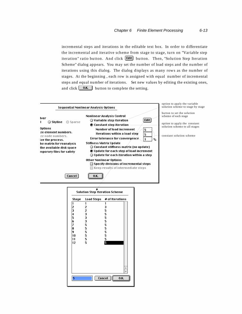
Chapter 6 Finite Element Processing 6-13
incremental steps and iterations in the editable text box. In order to differentiate
the incremental and iterative scheme from stage to stage, turn on "Variable step
iteration" ratio button. And click button. Then, "Solution Step Iteration
Scheme" dialog appears. You may set the number of load steps and the number of
iterations using this dialog. The dialog displays as many rows as the number of
stages. At the beginning , each row is assigned with equal number of incremental
steps and equal number of iterations. Set new values by editing the existing ones,
and click button to complete the setting.
constant solution scheme
button to set the solution scheme of each stage
option to apply the constantsolution scheme to all stages
option to apply the variable solution scheme to stage by stage

6-14 Chapter 6 Finite Element Processing
Processing of heat conduction and seepage analysis
P rocessing of heat conduction analysis is basically the same as that of stru c t u r a l
analysis. But a seepage analysis should go through iterative processes of
determining the phreatic flow surface which is not necessary in a structural or a
heat conduction analysis.
■ Setting analysis options for heat conduction analysis
A steady state analysis of a heat conduction problem re q u i res only one cycle of
equation assembly and solution process which is identical to the processing of a
linear static analysis of a structural problem. This type of processing is described
a l ready in "Processing of structural analysis" section of this chapter, and is not
repeated here.
■ Setting analysis options for seepage analysis
Although both the seepage analysis and the heat conduction analysis are based on
the same governing equations, the processing of seepage analysis is different from
that of the latter because it re q u i res an iterative pro c e d u re determining the
phreatic flow surface.
The editable text items of the dialog requires inputting the following values:
• Datum (Coordinate of zero height) : datum elevation. The hydraulic head is
set to 0 at this level.
direction of elevation(used only for 3-D models)
datum level H0
maximum head increment within an iteration cycle
convergence criterion for iteration(error percentage in head)
number of time steps (only for transient analysis)
length of a time step (only for transient analysis)
criterion for modifying the open head in each iteration
unit weight of fluid
maximum number of iterations

Chapter 6 Finite Element Processing 6-15
< Datum level>
• Unit weight of fluid : The unit weight of fluid is used in converting the head
to fluid pressure.• Number of time steps : the number of time steps involved
in the transient analysis. This value is ignored in a steady state analysis.
• Time step size : the length of time between two consecutive steps. This value
is ignored in a steady state analysis.
• Number of iteration within a step : The phreatic surface is determined by
iterative computation. This value specifies the maximum number of
iterations determining phreatic surface in a steady state analysis. This value
is also applied to a transient analysis as the number of iterations within each
time step.
• Error tolerance for convergence : Another criterion for finishing the iterative
p rocess is base on the maximum diff e rence of phreatic surface elevations
between the current and the last iterations. One of this and the above criteria
is met, the iterative processing is terminated.
• Open head increment : The limit of increment in modifying the open head in
a iteration cycle.
• Criterion for open head modification : The open head is incremented on the
basis of this criterion.
- "By elevation": If this option is on, the node with lowest elevation is searched
along the open head boundary, and the phreatic head is set to the head of
node. If more than one node has the lowest elevation, only the node with
the maximum pressure will be used to set the head
- "By pressure": If this option is on, he node with maximum positive pressure
is searched along the open head boundary, and the phreatic head is set to the
head of node.
X
H0 =Datum
H1
H2

6-16 Chapter 6 Finite Element Processing
Processing stages
Processing is divided into a few stages, and a message dialog shows the progress of
each stage. Processing can be interrupted or resumed in the middle, if necessary.
If there is any problem in solving the equations, appropriate message is displayed
and processing aborts.
■ Progress of processing
While the processing is going on, its pro g ress is indicated on a modal dialog as
shown below. The pro g ress is displayed in 3 stages. If the frontal solver is
adopted, “Assembling element”, “Back substitution”, and “Stress recovery and
smoothing” caption is posted on the dialog to indicate the processing stages. If
skyline solver is used, “Matrix decomposition” is posted at the second stage.
During the first stage, the element matrices are assembled. The dialog shows the
total number of elements as well as the number of elements assembled so far. For
nonlinear analysis or sequentially stage analysis, the stage No., the load
incremental step No. and the iteration No. are also displayed in the dialog. In case
of frontal solver, not only assembly but also decomposition of the equations are
going on at this stage.
Total number of elements
The number of the element now being assembled
stage No.
load incremental step No.
iteration No.
load incremental step No.
iteration No.
For linear analysis
For nonlinear analysis
For staged analysis
Chapter 6 Finite Element Processing 6-17
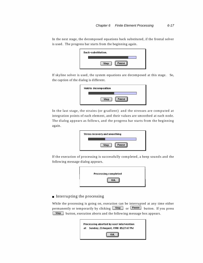
In the next stage, the decomposed equations back substituted, if the frontal solver
is used. The progress bar starts from the beginning again.
If skyline solver is used, the system equations are decomposed at this stage. So,
the caption of the dialog is different.
In the last stage, the strains (or gradient) and the stresses are computed at
integration points of each element, and their values are smoothed at each node.
The dialog appears as follows, and the pro g ress bar starts from the beginning
again.
If the execution of processing is successfully completed, a beep sounds and the
following message dialog appears.
■ Interrupting the processing
While the processing is going on, execution can be interrupted at any time either
permanently or temporarily by clicking or button. If you press
button, execution aborts and the following message box appears.

6-18 Chapter 6 Finite Element Processing
If you click button of the progress dialog, processing does not abort but is
temporarily suspended so that you may do other operations while the following
dialog stays on the screen.
Execution is resumed and the status dialog moves to the front when you click
button of the dialog. Processing may be aborted at this stage by pressing
button.
■ Abnormal termination of the processing
Processing may be terminated abnormally in the middle of execution due to one of
the following reasons.
• Matrix files for reanalysis are not found or are mismatching: If the solution
stage is set as “Reanalysis” but necessary files for reanalysis do not exist or do
not match the data file, the processing cannot be executed. So, the operation
will abort with the following message box.
The matrix files for reanalysis should reside in the same folder (or directory) as the
data file. And their name and extension should be compatible with that of the data
file. If the name of the data file is “mydata” , for example, “mydata.mtx” and
“mydata.fro” should exist in the same folder (or directory).
• I n s u fficient memory space: If “Skyline” is chosen as solver option, but the
CPU memory space is insufficient, then the software will let you to allow
automatic switch to “Frontal” as already explained in the previous section. In
case “Frontal” is chosen as solver option and the CPU memory space is
insufficient, the processing aborts with the following message box.

Chapter 6 Finite Element Processing 6-19
The re q u i red memory space for “Frontal” solver may be reduced by optimizing
element numbering. If a memory insufficiency problem persists even after element
number optimization, more computer memory should be secured for VisualFEA.
• Equation ill-conditioning: If the assembled system equations are ill-
conditioned, numerical difficulty arises in solving the equations, and thus the
processing aborts in the middle with the following message.
The possible causes of equation ill-conditioning are as follows.
- Poor element shape or element connectivity : The element stiffness matrix
may have numerical singularity due to unacceptably distorted shape or due
to improper connectivity. If such is the case, improve the element shape and
connectivity by carefully regenerating the finite element mesh again.
- I n s u fficient constraints : The system equations may have rank deficiency
due to insufficient constraints or boundary conditions. In this case, check
the boundary conditions and add more constraints if necessary.
- I r relevant element properties: Element stiffness matrices may have been
spoiled by irrelevant values of element properties. To avoid such problem,
check the contents of element property sets.
- insufficient integration order: The stiffness matrix may have spurious zero
e n e rgy modes due to insufficient integration ord e r. In order to re m o v e
spurious zero energy modes, adopt an integration scheme of higher order.

6-20 Chapter 6 Finite Element Processing
Interactive real time processing
VisualFEA has the capability of interactive real time processing for truss and frame
analysis. Interactive real time processing means that the cycle of data modification,
subsequent processing, and graphical visualization of the analysis results is formed
in real time. Thus, you can see the changing response as you add or modify the
data.
For analysis types of 2-D truss, 3-D truss, 2-D frame and 3-D frame,
interactive real time processing is the default mode. “Auto Solve” item of
menu is enabled only for these analysis types. The interactive real
time analysis mode can be turned on or off by checking the menu item. If
the mode is turned off, the normal pro c e d u re of processing applies, as
described in the previous sections.
If the mode is on, you don’t have to select “Solve” item from menu.
Instead, you have to designate the data item to display from
menu. Whenever you add or modify the data, the processing is executed
automatically, and the display of the analysis results is updated immediately.
The progress bar does not appear during processing.
F u r t h e r m o re, if “Instant Redrawing” item of menu is checked,
the diagrams re p resenting the analysis results are automatically updated
immediately after any change in the modeling data. Modification in
geometries, attributes, boundary conditions, or load conditions of the model
is reflected in the currently displayed diagram instantly.
An example of interactive real time analysis is shown in the following figure.
The example shows that the bending moment diagram is displayed directly
by selecting the corresponding menu item. There is no need to invoke
explicitly the processing stage. The diagram is updated at the moment the
load condition is altered. Likewise, the diagram will be changed as you
modify the boundary conditions or element properties. Thus, the responses
to varying external effects or attributes can be examined interactively.
On the other hand, interactive real time analysis may sometimes hamper the
responsiveness of the software, when the size of the problem is too large to get
enough speed in processing one cycle. In such circumstances, you may suppress
the options, by unchecking “Instant Redrawing” of menu. In addition,
the progress bar can be shown while processing goes on, if “Auto Solve” item of
menu is unchecked as well.

Chapter 6 Finite Element Processing 6-21
1. Model the structure, and assign attributes, boundary conditions and load conditions.
3. Bending moment diagram is displayed.
5. Select the point load.
2. Choose “Bending Moment” menu item.Make sure that “Instant Redrawing” item is also checked.
4. Choose “Load Condition” menu item.
6. Drag the point load to the right.Then, the bending moment diagram changes subsequently.
< Example of interactive real time processing>

6-22 Chapter 6 Finite Element Processing
Other Functions Related to Processing
The computational efficiency of processing depends on a number of factors like
node numbering, element numbering, integration scheme, and so on. They can be
manipulated to improve the efficiency.
Optimizing node numbering
If “S k y l i n e” solver is used, the re q u i red memory and the computing time is
d i rectly related to the band width of the system equations. The band width i s
determined by the node numbering. Therefore, node numbering is very important.
H o w e v e r, nodes are numbered initially in the order of their creation during the
modeling stage. It is desirable to renumber the nodes before processing stage so
that the band width is minimized. This pro c e d u re is called node number
optimization.
Node number optimization can be dictated as an optional item to be done before
processing as explained in the previous section. This option, however, may cause
redundant repetition of the operation, if the same modeling data are used for
multiple analysis. This redundant operation may be avoided by doing the node
number optimization once and executing the processing multiple times without
the optimization option.
Node number optimization can be invoked by choosing “Optimize Node Number”
item from the menu. A dialog shows the intermediate state of progressive band
width reduction and the final half band width (HBW) after the completion of
optimization. If you click button, the nodes will be re n u m b e red as
optimized. If you click button, the optimization is ignored and the old
node numbering will be retained. Save the file in order to keep this renumbering
for future processing.
It should be noted that the optimization does not mean absolute minimization of the band
width, but means relative reduction of the band width. There may exist a node numbering
with smaller band width than the optimized one. However, it is too time consuming or not
feasible to find the numbering with this absolute minimum band width.

Chapter 6 Finite Element Processing 6-23
Optimizing element numbering
If “Frontal” solver is used, the required memory and computing time are directly
related to the critical f rontal length of the system equations. The critical fro n t a l
length is determined by the element numbering. Similarly to node number
optimization, it is desirable to renumber the elements before processing stage so
that the critical frontal length becomes the minimum. This pro c e d u re is called
element number optimization.
Element number optimization can be dictated as an optional item to be done before
processing as explained in the previous section. This option, however, may cause
redundant repetition of the operation, if the same modeling data are used for
multiple analysis. This redundant operation may be avoided by doing the element
number optimization once and executing the processing multiple times without
optimization option.
Element number optimization can be invoked by choosing “Optimize Element
Number” item from menu. A dialog shows the intermediate state of progressive
reduction of critical frontal length and the final critical frontal length after
completion of optimization. If you click button, the elements will be
re n u m b e red as optimized. If you click button, the optimization is
ignored and the old element numbering will be retained. Save the file in order to
keep this renumbering for future processing.
It should be noted that the optimization does not mean absolute minimization of the critical
frontal length, but means relative reduction of the critical frontal length. There may exist
an element numbering with smaller critical frontal length than the optimized one.
However, it is too time consuming or not feasible to find the numbering with this absolute
minimum critical frontal length

6-24 Chapter 6 Finite Element Processing
Setting output items
• output items: Only the checked items are computed during the pro c e s s i n g
and accordingly are accessible for postprocessing or text output. Depending
on the subject of analysis, either structural analysis related items or heat
transfer related items are enabled and the others are disabled.
Specifying integration scheme
In order to change the integration scheme, select “Integration Scheme...” item from
menu. Then “Integration Scheme” dialog box appears as shown below.
Select the element shape (and order) from the popup menu of the dialog.
Then, alternative integration schemes for the element shape are displayed as radio
button items. The radio button corresponding to the current setting is marked.
The integration scheme can be changed simply by turning on the radio button of
Popup Menu Items
Element shape
Integration schemes
Either ‘Heat Analyis Items” or “Seepage Analysis Items” appearsdepending on coupling with the structural analysis.
Data of checked items are computed and savedfor text or graphic output.
The dimmed items indicate that the corresponding data are unavailable from the analysis.

Chapter 6 Finite Element Processing 6-25
the desired scheme. After changing the schemes of the relevant element shapes,
click button. The integration scheme of each element shape is applied in
computing the element stiffness matrix of the respective element shape.
VisualFEA uses numerical integration(Gauss quadrature) in evaluating the
s t i ffness matrix. The computing time, accuracy and stability of the system
equations depend greatly on the integration scheme. There are default schemes
p reset for various element shapes as shown in the following table. These
integration schemes can be altered if desired.
<Integration scheme>
Triangle
ElementShape
No. ofNodes
Integration Schemes
•
Quadrangle
Tetrahedron
Prism
Hexahedron
1
1
1
1
•
1
•
•
•
•
••
2×1
2×2×2
2×2
• •
••
3
4
•
••
•
•
•
•••
•
•••
•
5
2×3
3×3×3
3×3
••
••
•
•
•••
7
•
•
•••
•
•
•
••
••
•
•
•
•
•
•
•••••
••••••
••••••
••••••
••••
3
6
4
8
4
10
6
15
8
20
DefaultScheme
1
3
1
2×2
1
4
1
2×3
2×2×2
2×2×2

6-26 Chapter 6 Finite Element Processing
Displaying analysis information
The state of analysis and related information is displayed as exemplified below by
selecting “Analysis Info” item from menu. The information includes the
time and memory space required to solve the problem.
The above information is displayed only in case the problem was successfully
solved in the current session. If it was solved in the previous session, the
following message will be displayed.
If the problem has not gone through processing, the following message will be
shown.
If the processing was canceled in the middle, the following message will be
displayed .