Embed Size (px)
Citation preview

Civil Engineering Department: Engineering Statistics (ECIV 2005)
Engr. Yasser M. Almadhoun Page 1
Chapter 6: Descriptive Statistics
Problem (01): Make a frequency distribution table for the following data using 5 classes.
5 10 7 19 25 12 15 7 6 8
17 17 22 21 7 7 24 5 6 5
Solution:
≤ <
≤ <
≤ <
≤ <
≤ ≤
Problem (02): Annual Salaries Sample (in thousands of dollars) for municipal employees
in Los Angeles and Long Beach are listed.
Los Angeles 20.2 26.1 20.9 32.1 35.9 23 28.2 31.6 18.3
Long Beach 20.9 18.2 20.8 21.1 26.5 26.9 24.2 25.1 22.2
Find the number of classes and the class range, variance, and standard
deviation of each data set.
Solution:

Civil Engineering Department: Engineering Statistics (ECIV 2005)
Engr. Yasser M. Almadhoun Page 2
√9 = 3
Mean (�̅�) =∑ 𝑋
𝑛=
236.3
9= 26.26
Variance (𝑆2) =∑(𝑋 − �̅�)2
𝑛 − 1=
360.8241
9 − 1= 45.10
Standard deviation (𝑆) = √∑(𝑋 − �̅�)2
𝑛 − 1
= √360.8241
9 − 1
= √45.10
= 6.72
√9 = 3
Mean (�̅�) =∑ 𝑋
𝑛=
205.9
9= 22.88
Variance (𝑆2) =∑(𝑋 − �̅�)2
𝑛 − 1=
116.8209
9 − 1= 14.60
Standard deviation (𝑆) = √∑(𝑋 − �̅�)2
𝑛 − 1

Civil Engineering Department: Engineering Statistics (ECIV 2005)
Engr. Yasser M. Almadhoun Page 3
= √116.8209
9 − 1
= √14.60
= 3.82
Problem (03): The weights (in pounds) of the defensive players on a high school football
team are given.
(a) Make a boxplot of the data.
(b) Find the mode observation.
173 145 205 192 197 227 156 240 172 185
208 185 190 167 212 228 190 184 195
Solution:
Mean (�̅�) =∑ 𝑋
𝑛=
3651
19= 192.16

Civil Engineering Department: Engineering Statistics (ECIV 2005)
Engr. Yasser M. Almadhoun Page 4
Problem (04): The data set is the number of minutes a sample of 25 people exercise each
week.
108 139 120 123 120 132 123 131 131
157 150 124 111 101 135 119 116 117
127 128 139 119 118 114 127
(a) Make a frequency distribution of the data set using five classes.
Include class limits, midpoints, frequencies, boundaries, relative
frequencies, and cumulative frequencies.
(b) Display the data using a frequency histogram and a frequency
polygon on the same axes.
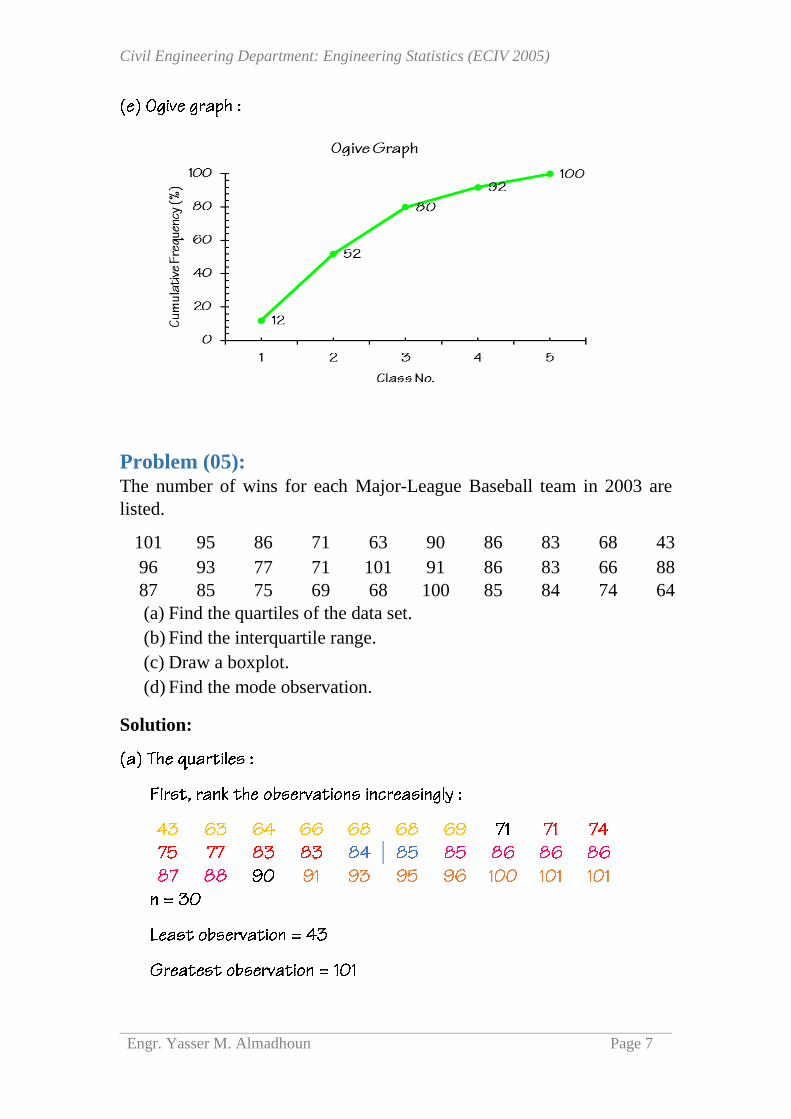
(c) Display the data using a relative frequency histogram.
(d) Display the data using a boxplot.
(e) Display the data using an ogive
Solution:
Least
observation
Lower
quartile Median Upper
quartile Greatest
observation
Mean
Interquartile range
145.0 173.0 208.0 190.0
240.0
35.0 192.16

Civil Engineering Department: Engineering Statistics (ECIV 2005)
Engr. Yasser M. Almadhoun Page 5
≤ <
≤ <
≤ <
≤ <
≤ ≤
Civil Engineering Department: Engineering Statistics (ECIV 2005)
Engr. Yasser M. Almadhoun Page 6
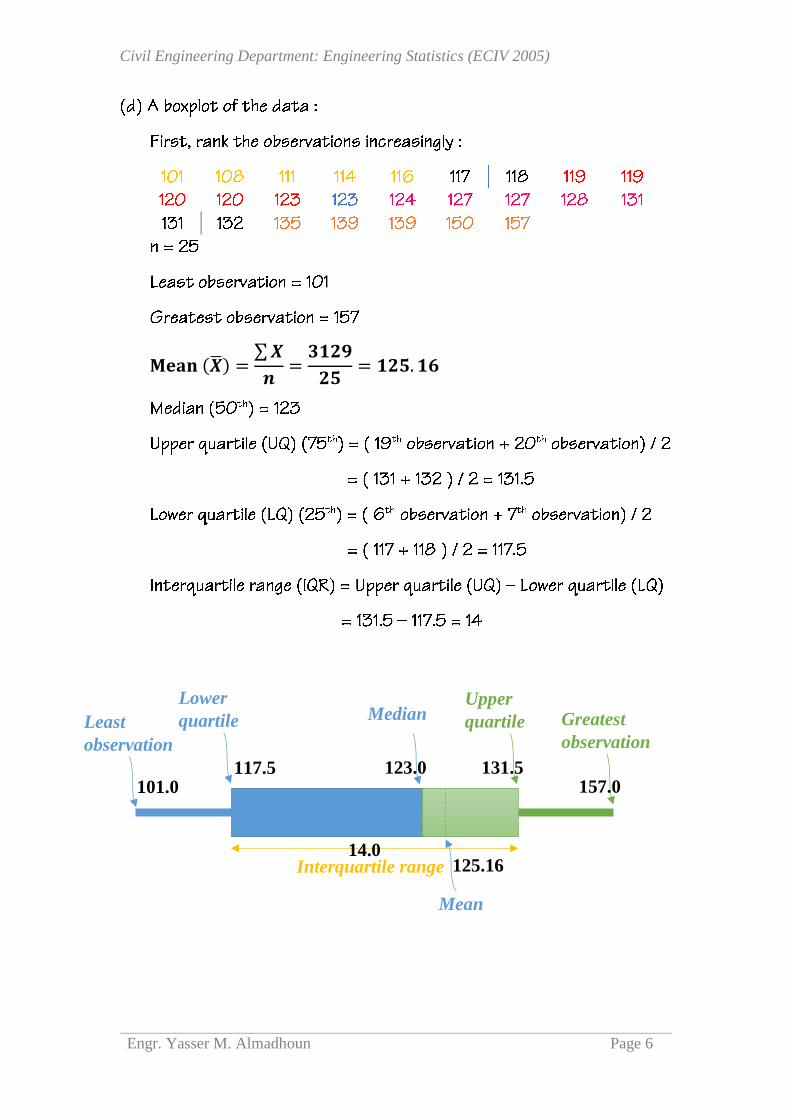
𝐌𝐞𝐚𝐧 (�̅�) =∑ 𝑿
𝒏=
𝟑𝟏𝟐𝟗
𝟐𝟓= 𝟏𝟐𝟓. 𝟏𝟔
Least
observation
Lower
quartile Median Upper
quartile Greatest
observation
Mean
Interquartile range
101.0 117.5 131.5 123.0
157.0
14.0 125.16
Civil Engineering Department: Engineering Statistics (ECIV 2005)
Engr. Yasser M. Almadhoun Page 7
Problem (05): The number of wins for each Major-League Baseball team in 2003 are
listed.
101 95 86 71 63 90 86 83 68 43
96 93 77 71 101 91 86 83 66 88
87 85 75 69 68 100 85 84 74 64
(a) Find the quartiles of the data set.
(b) Find the interquartile range.
(c) Draw a boxplot.
(d) Find the mode observation.
Solution:

Civil Engineering Department: Engineering Statistics (ECIV 2005)
Engr. Yasser M. Almadhoun Page 8
Mean (�̅�) =∑ 𝑋
𝑛=
2429
30= 80.97
Problem (06): For the following set of data, using five classes, find:
87 82 64 95 66 75 88 92 67 77 71 76
93 88 75 55 69 87 61 94 87 74 66 92
69 77 92 83 85 90 65 74 84 65 91 70
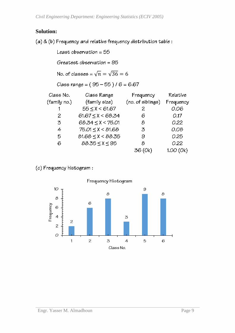
(a) The frequency distribution table.
(b) The relative frequency distribution table.
(c) The Frequency Histogram.
(d) Present the data as stem-and-leaf plot.
Least
observation
Lower
quartile Median Upper
quartile Greatest
observation
Mean
Interquartile range
43.0 71.75 90.0 84.5
101.0
19.0 80.97
Civil Engineering Department: Engineering Statistics (ECIV 2005)
Engr. Yasser M. Almadhoun Page 9
Solution:
√𝑛 = √36 = 6
≤ <
≤ <
≤ <
≤ <
≤ <
≤ ≤

Civil Engineering Department: Engineering Statistics (ECIV 2005)
Engr. Yasser M. Almadhoun Page 10
Problem (07): The grades of 20 students in statistics midterm exam are as follow:
30 21 15 14 10
19 14 22 27 30
20 18 23 15 16
16 15 29 28 13
(a) Calculate the sample mean and the trimmed mean.
(b) Calculate the sample standard deviation.
(c) Find the quartiles.
(d) Draw a boxplot of the above data set.
(Question 6: in Final Exam 2005)
Solution:
Mean (�̅�) =∑ 𝑋
𝑛=
395
20= 19.75

Civil Engineering Department: Engineering Statistics (ECIV 2005)
Engr. Yasser M. Almadhoun Page 11
Trimmed mean (𝑋𝑇10%̅̅ ̅̅ ̅̅ ̅̅ ) =
∑ 𝑋
𝑛=
312
16= 19.50
𝑋 (𝑋 − �̅�) (𝑋 − �̅�)2
Variance (𝑆2) =∑(𝑋 − �̅�)2
𝑛 − 1=
739.75
20 − 1= 38.93
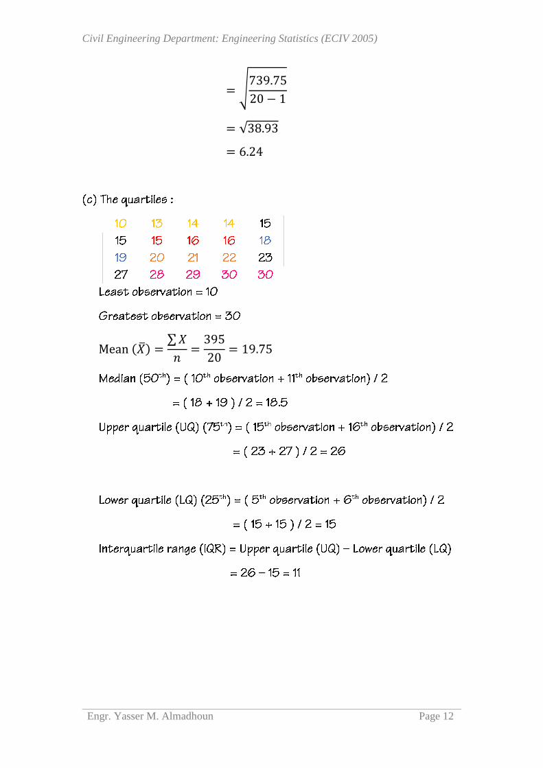
Standard deviation (𝑆) = √∑(𝑋 − �̅�)2
𝑛 − 1
Civil Engineering Department: Engineering Statistics (ECIV 2005)
Engr. Yasser M. Almadhoun Page 12
= √739.75
20 − 1
= √38.93
= 6.24
Mean (�̅�) =∑ 𝑋
𝑛=
395
20= 19.75

Civil Engineering Department: Engineering Statistics (ECIV 2005)
Engr. Yasser M. Almadhoun Page 13
Problem (08): Use the boxplot below to determine which statement is accurate (choose
the best alternative):
(a) About 25% of the adults have cholesterol levels of at most 211.
(b) About 75% of the adults have cholesterol levels less than 180.
(c) One half of the cholesterol levels are between 180 and 197.5.
(d) One half of the cholesterol levels are between 180 and 211.
Solution:
Smaller
observation
Lower
quartile Median Upper
quartile Greatest
observation
Mean
Interquartile range
10.0 15.0 26.0 18.5
30.0
11.0 19.75