Chapter 6 Cost analysis Chapter 6 Cost analysis and Measurementand Measurement

Chapter 6 Cost analysis Chapter 6 Cost analysis and Measurementand Measurement

KEY CONCEPTS• historical cost• current cost• replacement cost• opportunity cost• explicit cost• implicit cost• incremental cost• profit contribution• sunk cost• cost function• short-run cost functions• long-run cost functions• planning curves

• operating curves fixed cost• variable cost• short-run cost curve• long-run cost curve• economies of scale• cost elasticity• capacity• minimum efficient scale• multiplant economies of scale• multiplant diseconomies of scale• learning curve• economies of scope• cost-volume-profit analysis• breakeven quantity

OVERVIEW

• What Makes Cost Analysis Difficult• Opportunity Cost• Incremental and Sunk Costs in Decision

Analysis• Short-run and Long-run Costs• Short-run Cost Curves• Long-run Cost Curves• Minimum Efficient Scale• Firm Size and Plant Size• Learning Curves• Economies of Scope• Cost-volume-profit Analysis

一 . Nature of costs

• 1.Accounting cost and Economic cost

2. Historical costs Versus Current Costs

Historical cost: the actual cash outlay

Current cost: the present cost of previously acquired items

3.Replacement Cost– Cost of replacing productive capacity

using current technology.

• 4.Opportunity Cost – foregone value.– second-best use.

• 5.Explicit and Implicit Costs– Explicit costs= cash expenses– Implicit costs= noncash

expenses

• 6.Incremental Cost and marginal cost– Incremental cost: the change in cost

tied to a managerial decision.– Incremental cost can involve multiple

units of output.

Marginal cost: a single unit of output.

• 7.Sunk Cost– Irreversible expenses incurred

previously.

– **Sunk costs are irrelevant to present decisions.

Definition of the Operating Period– At least one input is fixed in the

S.R.– All inputs are variable in the L.R.

• Fixed and Variable Costs

二 .Short-run Costs1.Categories: Total Cost = Fixed Cost + Variable

Cost– ATC = AFC + AVC– MC = ∂TC/∂Q

2. Cost curves**Short-run Cost Relations

– Short-run cost curves show minimum cost in a given production environment.

True or false:1. An implicit cost usually involves the

use of resources owned by the owner of the firm.

2. Costs are money payments for the use of resources.

3. Variable costs depend on how much output is produced.

4. Short run is a period of time that is less than 1 year.

??List the inputs that generate explicit costs and implicit costs

• A self-employed automobile mechanic uses his own tools, rents a building, buys replacement parts, and hires a teenager as a helper.

•??opportunity cost• A piece of land is used to raise

wheat . If the farmer could make $2000 by growing corn on this land, $1800 by growing peanuts, $1700 by growing soybeans, and $1500 by raising cattle, what is the opportunity cost of the wheat.

Which of the following are short‑run and which are long‑run adjustments?

(a) Wendy’s builds a new restaurant;(b) Acme Steel Corporation hires 200

more production workers; (c) A farmer increases the amount of

fertilizer used on his corn crop; (d) An Alcoa plant adds a third shift of

workers.

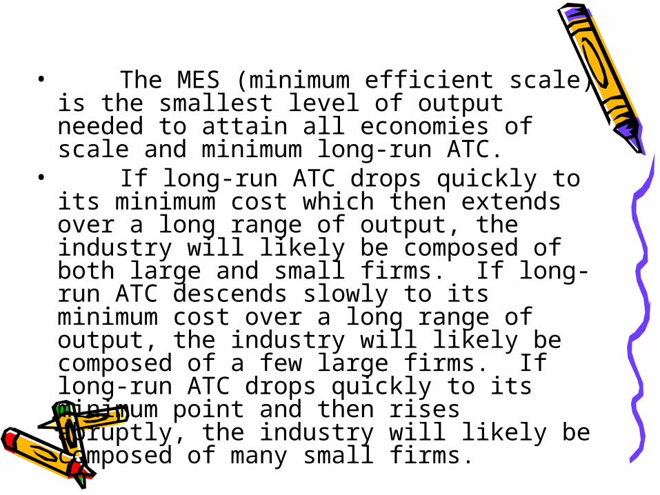
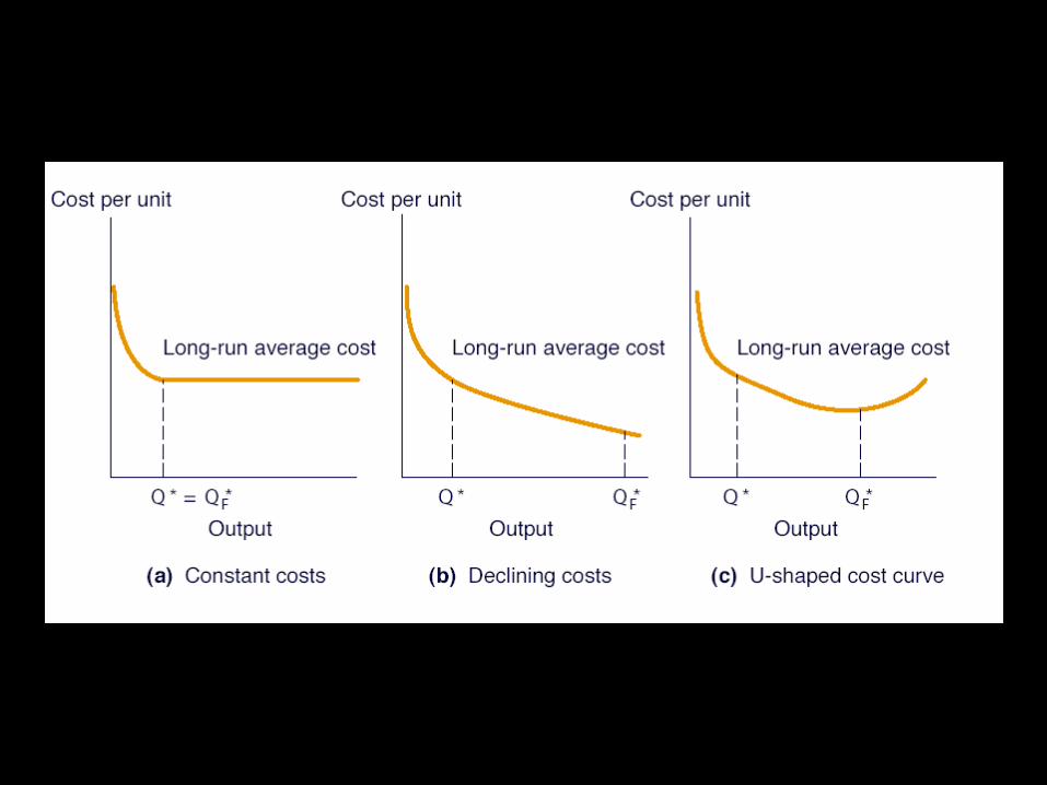
• The MES (minimum efficient scale) is the smallest level of output needed to attain all economies of scale and minimum long-run ATC.

• If long-run ATC drops quickly to its minimum cost which then extends over a long range of output, the industry will likely be composed of both large and small firms. If long-run ATC descends slowly to its minimum cost over a long range of output, the industry will likely be composed of a few large firms. If long-run ATC drops quickly to its minimum point and then rises abruptly, the industry will likely be composed of many small firms.

三 .Long-run Cost Curves

• 1.Types of LR costs• 2.LRAC and SRAC( envelope of

SACs) • 3.law • 4. economy of scale/diseconomies

of scale• 5. minimum efficient scale• ６ .shift of long run cost curve:

learning curve• 7. break even analysis

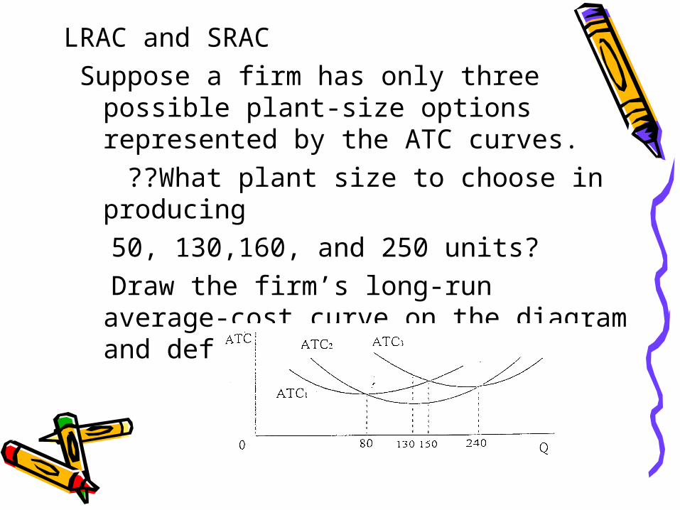
LRAC and SRAC Suppose a firm has only three possible

plant-size options represented by the ATC curves.

??What plant size to choose in producing

50, 130,160, and 250 units? Draw the firm’s long‑run average‑cost

curve on the diagram and define this curve.

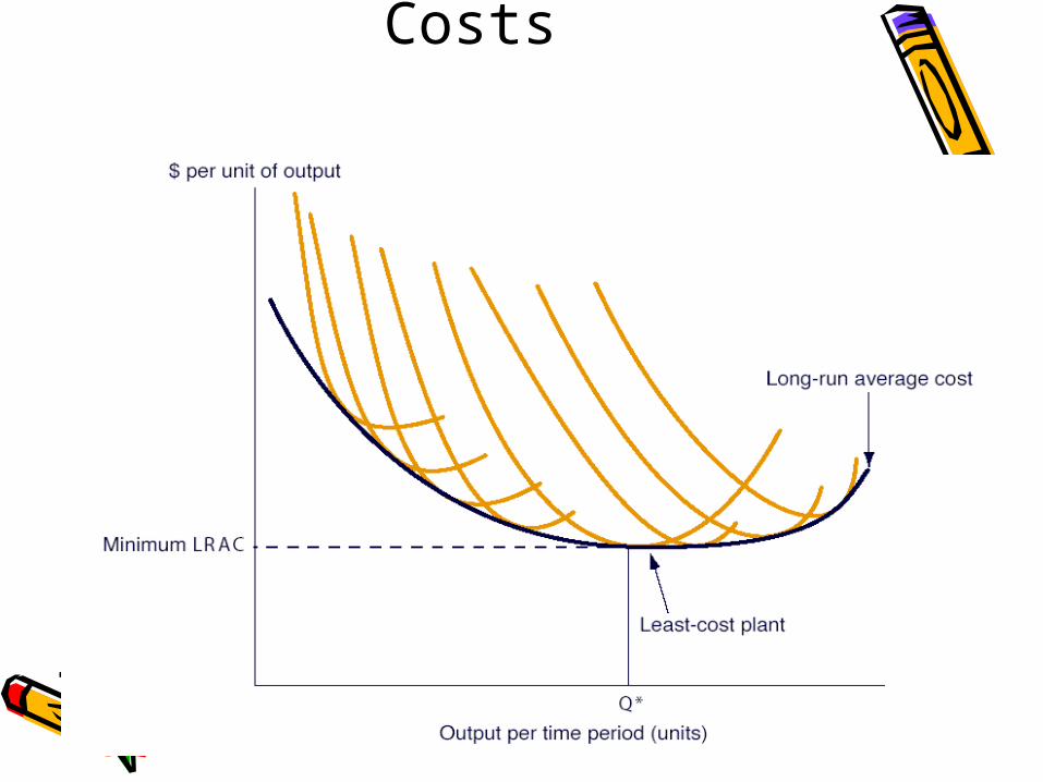
Long-run Average Costs

To understand LRAC

• LRAC: shows the lowest average total cost at which any output level can be produced after the firm has had time to make all appropriate adjustments in its plant size.

??Why U-shaped LRAC

Law--AC

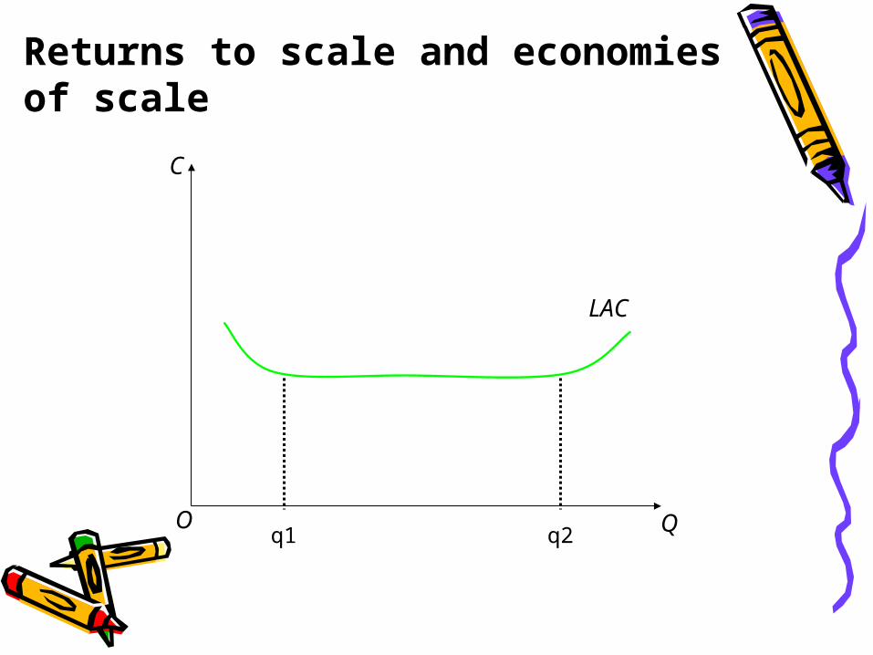
• Economies of scale: the reduction in LRAC as the scale of the firm’s output is increased.

• Diseconomies of scale:

O

C

Q

LAC

q1 q2

Returns to scale and economies of scale

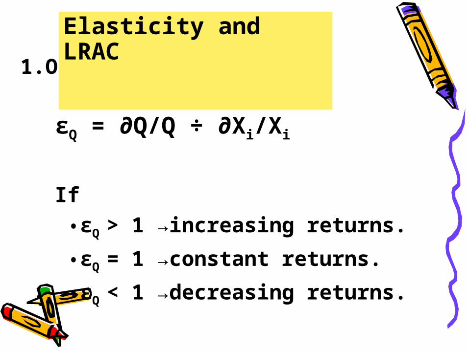
1.Output Elasticity

εQ = ∂Q/Q ÷ ∂Xi/Xi

If

•εQ > 1 →increasing returns.

•εQ = 1 →constant returns.

•εQ < 1 →decreasing returns.

Elasticity and LRAC

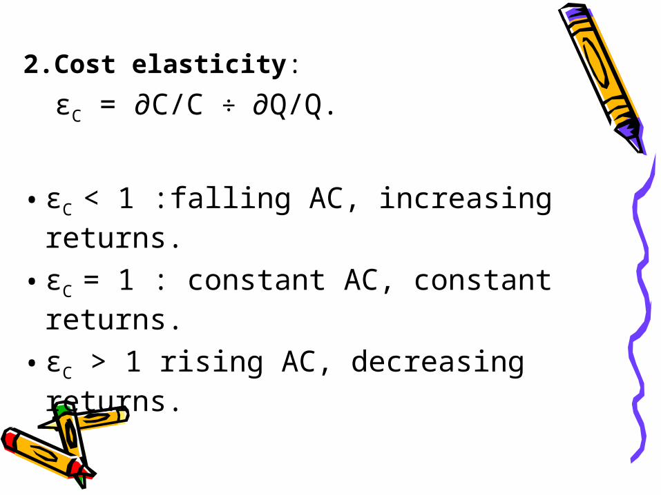
2.Cost elasticity:

εC = ∂C/C ÷ ∂Q/Q.

• εC < 1 :falling AC, increasing returns.

• εC = 1 : constant AC, constant returns.

• εC > 1 rising AC, decreasing returns.

5.Minimum Efficient Scale

Definition of MES: output level at the minimum point on the LRAC curve.

Competitive Implications of MES:

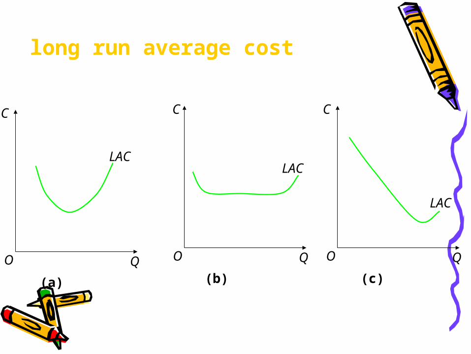
long run average cost

O

C

Q

LAC

(a)

O

C

Q

LAC

(b)

O

C

Q

LAC

(c)

6.Learning Curves

• Definition : average cost reduction over time due to production experience.

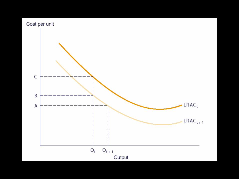
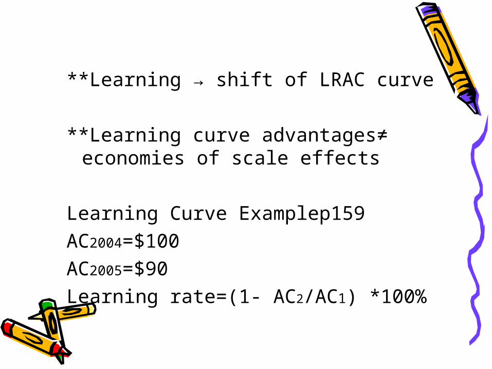
**Learning → shift of LRAC curve

**Learning curve advantages≠ economies of scale effects

Learning Curve Examplep159AC2004=$100AC2005=$90Learning rate=(1- AC2/AC1) *100%

• Strategic Implications of the Learning Curve Concept– When learning results in 20% to 30%

cost savings, it becomes a key part of competitive strategy.

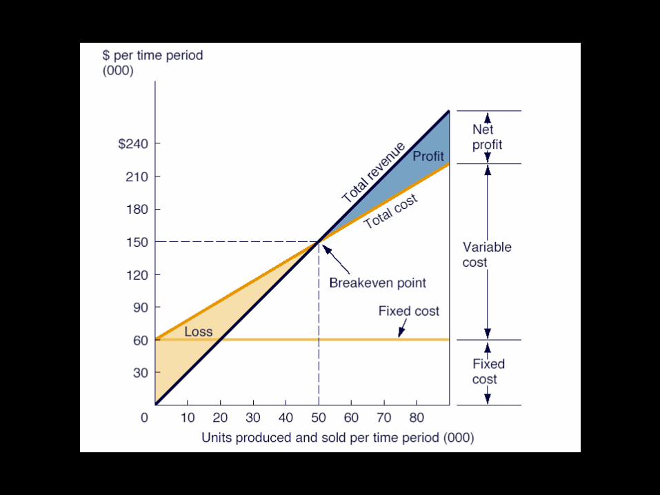
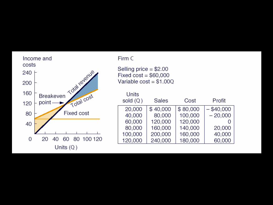
7.Cost-volume-profit Analysis

• (1) ． Break even quantity

• 　 QBE=TFC/ (P-AVC)　• 　　 Example

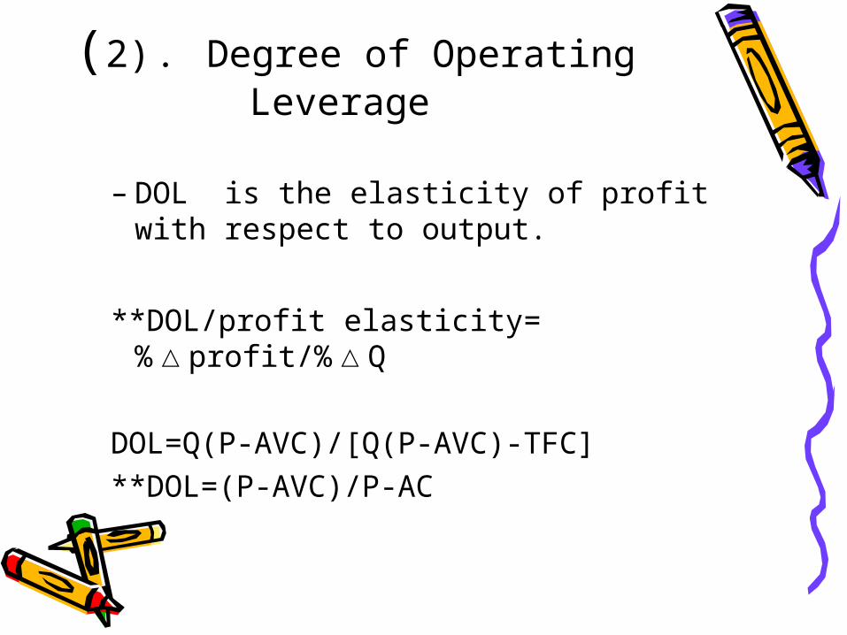
(2) ． Degree of Operating Leverage

– DOL is the elasticity of profit with respect to output.

**DOL/profit elasticity= %△profit/%△Q

DOL=Q(P-AVC)/[Q(P-AVC)-TFC]**DOL=(P-AVC)/P-AC

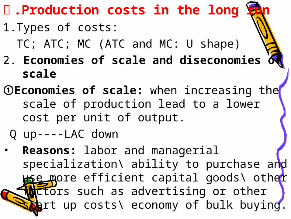
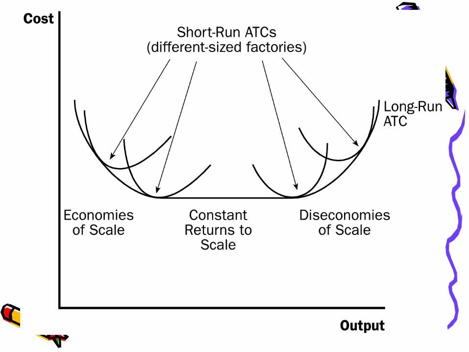
五 .Production costs in the long run1.Types of costs: TC; ATC; MC (ATC and MC: U shape)2. Economies of scale and diseconomies of

scale①Economies of scale: when increasing the

scale of production lead to a lower cost per unit of output.

Q up----LAC down• Reasons: labor and managerial

specialization\ ability to purchase and use more efficient capital goods\ other factors such as advertising or other start up costs\ economy of bulk buying.

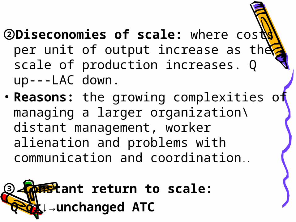
②Diseconomies of scale: where costs per unit of output increase as the scale of production increases. Q up---LAC down.

• Reasons: the growing complexities of managing a larger organization\ distant management, worker alienation and problems with communication and coordination..

③ Constant return to scale: Q↑or↓→unchanged ATC

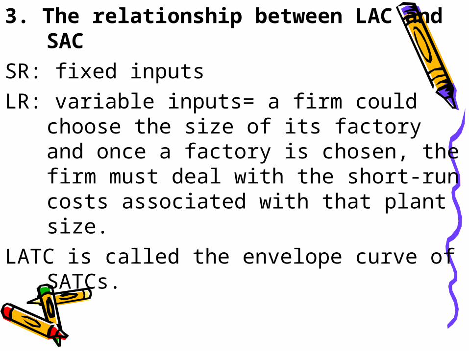
3. The relationship between LAC and SAC

SR: fixed inputsLR: variable inputs= a firm could choose

the size of its factory and once a factory is chosen, the firm must deal with the short-run costs associated with that plant size.

LATC is called the envelope curve of SATCs.

4.Minimum efficient scale and industry structure

Minimum efficient scale: MECthe smallest level of output at which a firm

can minimize its average costs in the long run..

If the MES is a large percentage of the market, and if the firms are to be large enough to gain the full economies of scale, there will not be room for many firms.

If the MES exceeds 50%, there is only room for one firm large to gain full economies of scale. In this case, the industry is said to be a natural monopoly.

• **MES +market==structure

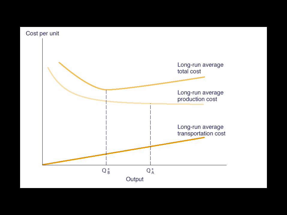
Transportation Costs and MES

– Terminal, line-haul and inventory costs can be important.

– High transport costs reduce MES impact.

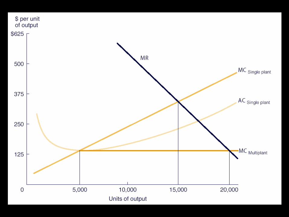
Firm Size and Plant Size

• Multi-plant Economies and Diseconomies of Scale– Multi-plant economies are cost

advantages from operating several plants.

– Multi-plant diseconomies are cost disadvantages from operating several plants.

Economics of Multi-plant Operation: an Example

• Plant Size and Flexibility

Economies of Scope• Economies of Scope Concept

– Scope economies are cost advantages that stem from producing multiple outputs.

– Big scope economies explain the popularity of multi-product firms.

– Without scope economies, firms specialize.

• Exploiting Scope Economies– Scope economics often shape competitive

strategy for new products.