Embed Size (px)
Citation preview
113
Chapter 6
6. Control of Shunt Active Filter
6.1 Introduction
The SAF generates a current equal and opposite to the load current
harmonics and reactive power component at fundamental frequency to
achieve balanced, sinusoidal supply current which is in phase with the
voltage at PCC. The critical task of the SAF controller is to generate reference
current. The accuracy of the SAF current reference determines performance
of SAF. Reference current generation methods utilized in SAF applications
can summarized in two groups as frequency domain methods and time
domain methods. Frequency domain methods are based on Fourier analysis.
The time domain methods are more preferred over the former due to
less number of calculations and fast response during transients. There exist
two well known time domain methods of harmonic extraction in SAF appli-
cation based on: 1) Instantaneous reactive power (IRP) theory 2) Synchronous
reference frame theory (SRF), briefly introduced in Chapter 1. A review of the
two techniques is presented in next section. A method to extract SAF refer-
ence current based on SSI (Sine Signal Integrator) for single phase SAF
application is presented in this chapter. This technique is particularly suited
for single phase applications as it simplifies the task of generating orthogonal
signal which is a main hurdle in extracting reference current for single phase
SAF using IRP and SRF techniques.

Chapter 6. Control of Shunt Active Filter
114
The current controller controls switching of the VSI switches so that the
current injected by the VSI is exactly equal to the reference current. A review
of different current control techniques and M-PWM (modified PWM) current
control technique is also explained.
In spite of compensation of harmonic currents of the load, SAF leaves
switching frequency ripple in the supply current if not filtered. This requires
a switching ripple filter at the input of SAF. Design of a broad-band tuned
type switching ripple filter is presented at the end.
6.2 Instantaneous Reactive Power Theory (p-q theory)
The p-q theory proposed by Akagi et. al. [H1] deals with instantaneous
powers. It is based on abc to 0 transformation to calculate instantaneous
powers defined in the time domain. As it is instantaneous, it assumes no
restrictions on the voltage and current waveforms. It is not only valid in
steady state but also in transient state. It can be applied to three phase sys-
tems with or without neutral wire. p-q theory has made it possible to design
very efficient and flexible controllers for power quality conditioners based on
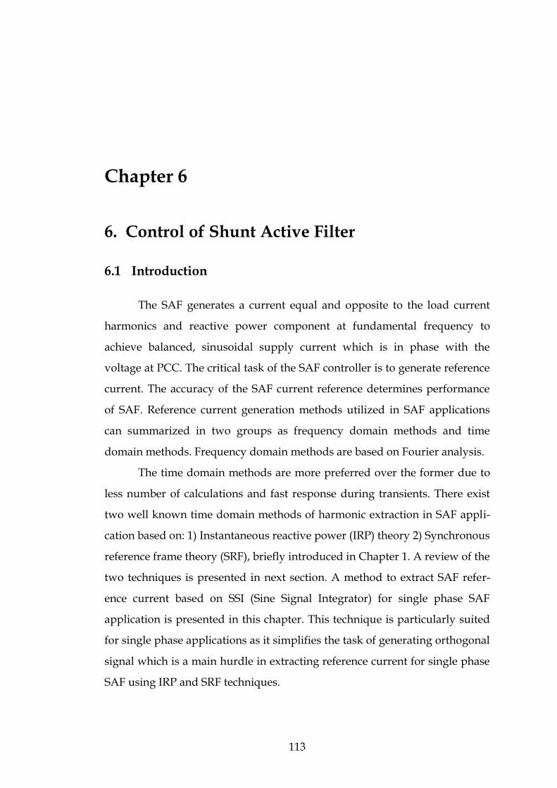
power electronic devices. Fig. 6.1 illustrates basic idea of three phase shunt
current compensation. It is assumed that the compensator behaves like a
controlled current source that can draw arbitrary chosen current references*cai , *
cbi , *cci . Fig. 6.2 shows a general controller structure[H1,J5]. The calculated
real and imaginary powers p, q of the load can be separated into its average (
,p q ) and oscillating ( ,p q ) parts respectively. Then the undesired portions of
real and imaginary powers of the load that should be compensated are
selected and compensating powers * *,c cp q are derived. The negative sign
implies compensating current being exact inverse of the corresponding
undesired component of the load current. The inverse transformation from
0 to abc is applied to calculate instantaneous value of the compensating
current references *cai , *
cbi , *cci .
Chapter 6. Control of Shunt Active Filter
115
Figure 6-2 Control method for three phase shunt compensation based on p-q theory
The merits and drawbacks of p-q theory are reported as [H2] as: 1) easy
implementation 2) excellent steady state performance and the drawback
being sensitivity to harmonics and unbalances in the supply voltage [H17].
Figure 6-1: Basic shunt compensation principle
Chapter 6. Control of Shunt Active Filter
116
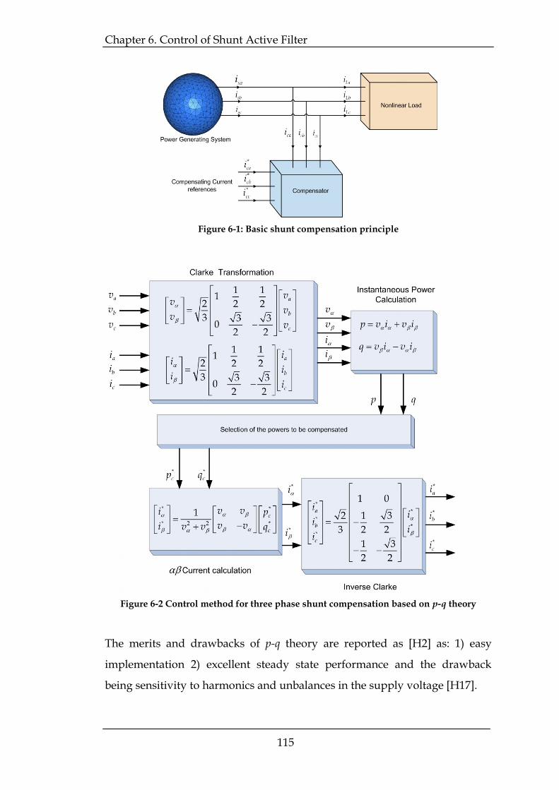
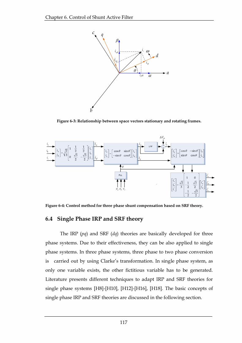
6.3 Synchronous Reference Frame Theory (dq theory)
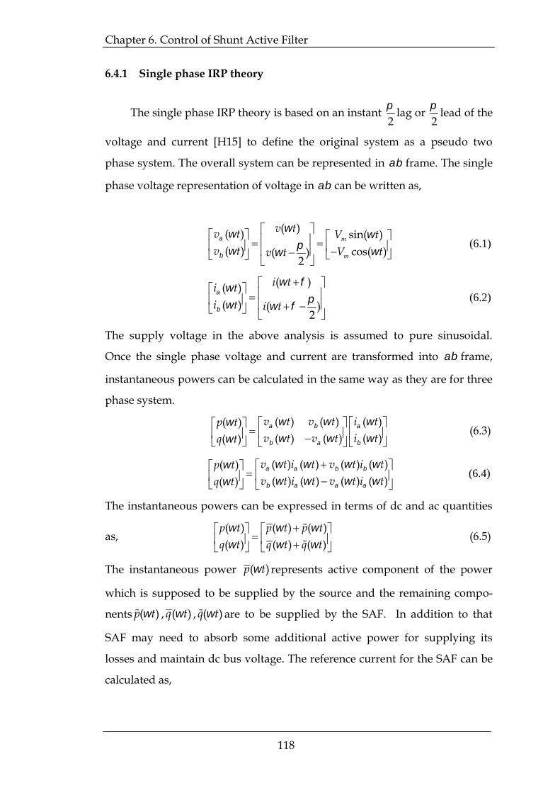
The basic principle of synchronous reference frame controller [H2] for
the current reference generation in SAF is illustrated in Fig. 6.4. The meas-
ured load currents in abc reference frame are first transformed into frame
via abc- transformation and subsequently to synchronous reference frame
(dq) reference frame via to dq transformation. The to dq transformation
utilizes phase angle information ( t ) of the utility voltage for the transfor-
mation of the quantities to synchronous rotating frame. The and dq
frames are illustrated in Fig. 6.3. In synchronous rotating frame, once the
transformation is carried out, the positive sequence components at funda-
mental frequency appear as dc quantities whereas negative sequence
components at and other frequency components (harmonics) appear as ac.
By employing proper filtering technique in the dq reference frame, the dc and
ac quantities can be easily separated. Once the filtering in the dq reference is
carried out, the desired dq reference signals are obtained and transformed
back to . The three phase current references can be obtained via to dq
transformation.
One important characteristics of the SRF theory is that the reference
currents are directly obtained from the load current without considering the
source voltage. This is an important advantage since the generation of refer-
ence current is not affected by supply voltage unbalance or distortion.
However, in order to transform to dq synchronous rotating frame, sine
and cosine signals synchronized with the respective phase-to-neutral supply
voltages are required. A phase locked loop (PLL) must be used to derive sine
and cosine signals corresponding to the supply voltage. A novel PLL and its
performance are also presented later in this chapter.
Chapter 6. Control of Shunt Active Filter
117
6.4 Single Phase IRP and SRF theory
The IRP (pq) and SRF (dq) theories are basically developed for three
phase systems. Due to their effectiveness, they can be also applied to single
phase systems. In three phase systems, three phase to two phase conversion
is carried out by using Clarke’s transformation. In single phase system, as
only one variable exists, the other fictitious variable has to be generated.
Literature presents different techniques to adapt IRP and SRF theories for
single phase systems [H8]-[H10], [H12]-[H16], [H18]. The basic concepts of
single phase IRP and SRF theories are discussed in the following section.
Figure 6-3: Relationship between space vectors stationary and rotating frames.
Figure 6-4: Control method for three phase shunt compensation based on SRF theory.
Chapter 6. Control of Shunt Active Filter
118
6.4.1 Single phase IRP theory
The single phase IRP theory is based on an instant2 lag or
2 lead of the
voltage and current [H15] to define the original system as a pseudo two
phase system. The overall system can be represented in frame. The single
phase voltage representation of voltage in can be written as,
( )( ) sin( )( ) cos( )( )
2
m
m
v tv t V tv t V tv t
(6.1)
( )( )( ) ( )
2
i ti ti t i t
(6.2)
The supply voltage in the above analysis is assumed to pure sinusoidal.
Once the single phase voltage and current are transformed into frame,
instantaneous powers can be calculated in the same way as they are for three
phase system.
( ) ( ) ( )( )( ) ( ) ( )( )
v t v t i tp tv t v t i tq t
(6.3)
( ) ( ) ( ) ( )( )( ) ( ) ( ) ( )( )
v t i t v t i tp tv t i t v t i tq t
(6.4)
The instantaneous powers can be expressed in terms of dc and ac quantities
as,( ) ( ) ( )( ) ( ) ( )
p t p t p tq t q t q t
(6.5)
The instantaneous power ( )p t represents active component of the power
which is supposed to be supplied by the source and the remaining compo-
nents ( )p t , ( )q t , ( )q t are to be supplied by the SAF. In addition to that
SAF may need to absorb some additional active power for supplying its
losses and maintain dc bus voltage. The reference current for the SAF can be
calculated as,
Chapter 6. Control of Shunt Active Filter
119
*
* 2 2
( ) ( ) ( )( ) 1( ) ( ) ( )( ) ( ) ( )
c v t v t p ti tv t v t q ti t v t v t
(6.6)
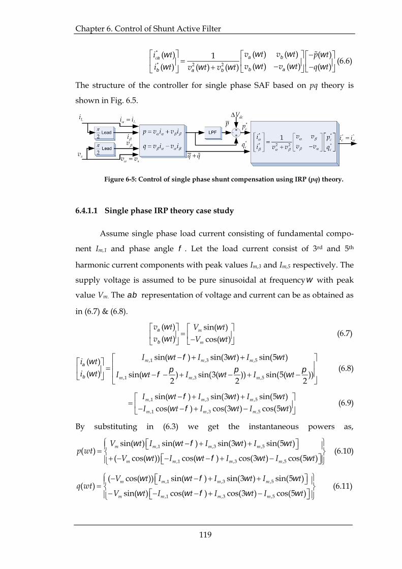
The structure of the controller for single phase SAF based on pq theory is
shown in Fig. 6.5.
6.4.1.1 Single phase IRP theory case study
Assume single phase load current consisting of fundamental compo-
nent Im,1 and phase angle . Let the load current consist of 3rd and 5th
harmonic current components with peak values Im,3 and Im,5 respectively. The
supply voltage is assumed to be pure sinusoidal at frequency with peak
value Vm. The representation of voltage and current can be as obtained as
in (6.7) & (6.8).
( ) sin( )( ) cos( )
m
m
v t V tv t V t
(6.7)
,1 ,3 ,5
,1 ,3 ,5
sin( ) sin(3 ) sin(5 )( )( ) sin( ) sin(3( )) sin(5( ))
2 2 2
m m m
m m m
I t I t I ti ti t I t I t I t
(6.8)
,1 ,3 ,5
,1 ,3 ,5
sin( ) sin(3 ) sin(5 )cos( ) cos(3 ) cos(5 )
m m m
m m m
I t I t I tI t I t I t
(6.9)
By substituting in (6.3) we get the instantaneous powers as,
,1 ,3 ,5
,1 ,3 ,5
sin( ) sin( ) sin(3 ) sin(5 )( )
( cos( )) cos( ) cos(3 ) cos(5 )m m m m
m m m m
V t I t I t I tp wt
V t I t I t I t
(6.10)
,1 ,3 ,5
,1 ,3 ,5
( cos( )) sin( ) sin(3 ) sin(5 )( )
sin( ) cos( ) cos(3 ) cos(5 )m m m m
m m m m
V t I t I t I tq wt
V t I t I t I t
(6.11)
Figure 6-5: Control of single phase shunt compensation using IRP (pq) theory.
Chapter 6. Control of Shunt Active Filter
120
Solving further,
,1 ,3 ,5( ) cos( ) cos(4 ) cos(4 )m m m m m mp wt V I V I t V I t (6.12)
,1 ,3 ,5( ) sin( ) sin(4 ) sin(4 )m m m m m mq wt V I V I t V I t (6.13)
The oscillating active power can be represented as,
,3 ,5( ) cos(4 ) cos(4 )m m m mp wt V I t V I t (6.14)
*,3 ,5( ) 1( cos(4 ) cos(4 ))c m m m mp wt V I t V I t (6.15)
*,1 ,3 ,5( ) 1( sin( ) sin(4 ) sin(4 ))c m m m m m mq wt V I V I t V I t (6.16)
The SAF reference current can be derived from (6.6) above,
,3 ,5*2
,1 ,3 ,5
sin( ) cos(4 ) cos(4 )1( )cos( ) ( sin( ) sin(4 ) sin(4 ))
m m m m m
m m m m m m m m
V t V I t V I ti t
V V t V I V I t V I t
(6.17)
*,1 ,3 ,5( ) 1 sin( )cos( ) sin(3 ) sin(5 )m m mi t I t I t I t (6.18)
The SAF reference current derived from application of IRP theory is such that
the resulting instantaneous active power is constant as seen by the supply
side. This means that the SAF will compensate for the oscillating component
of the load active power, p wt( ) and reactive power component, q wt( ) . As
stated in [H17], the SAF controlled according to the IRP theory, in the pres-
ence of supply voltage harmonics “attempts” to compensate even an ideal,
resistive, unity-power factor load and the compensator injects a distorted
current into the supply system unnecessarily. In the present work, a method
based on SSI is used to extract fundamental component of supply voltage
before calculating instantaneous active and reactive powers as per IRP
theory.
6.4.2 Single phase SRF theory
In order to apply the concept of dq transformation for single phase
systems, the basic requirement is representation of single phase system in
reference frame. As stated previously, it requires a phase shift of2 in the
original variable to generate the component. The resulting equations in dq
reference frame can be stated as,
Chapter 6. Control of Shunt Active Filter
121
( ) ( )sin( ) cos( )( ) ( )cos( ) sin( )
d
q
i t i tt ti t i tt t
(6.19)
( ) ( )( ) ( )sin( ) ( )cos( )( ) ( )cos( ) ( )sin( )( ) ( )
d dd
q q q
i t i ti t i t t i t ti t i t t i t ti t i t
(6.20)
The dc terms in (6.20), ( )di t and ( )qi t represents fundamental active and
reactive current components of the load and the non-dc terms, ( )di t and
( )qi t represents harmonic components of active and reactive current. The dc
terms from ( )di t and ( )qi t can be easily extracted by using a low pass filter.
The current reference in dq domain is generated by subtracting the dc com-
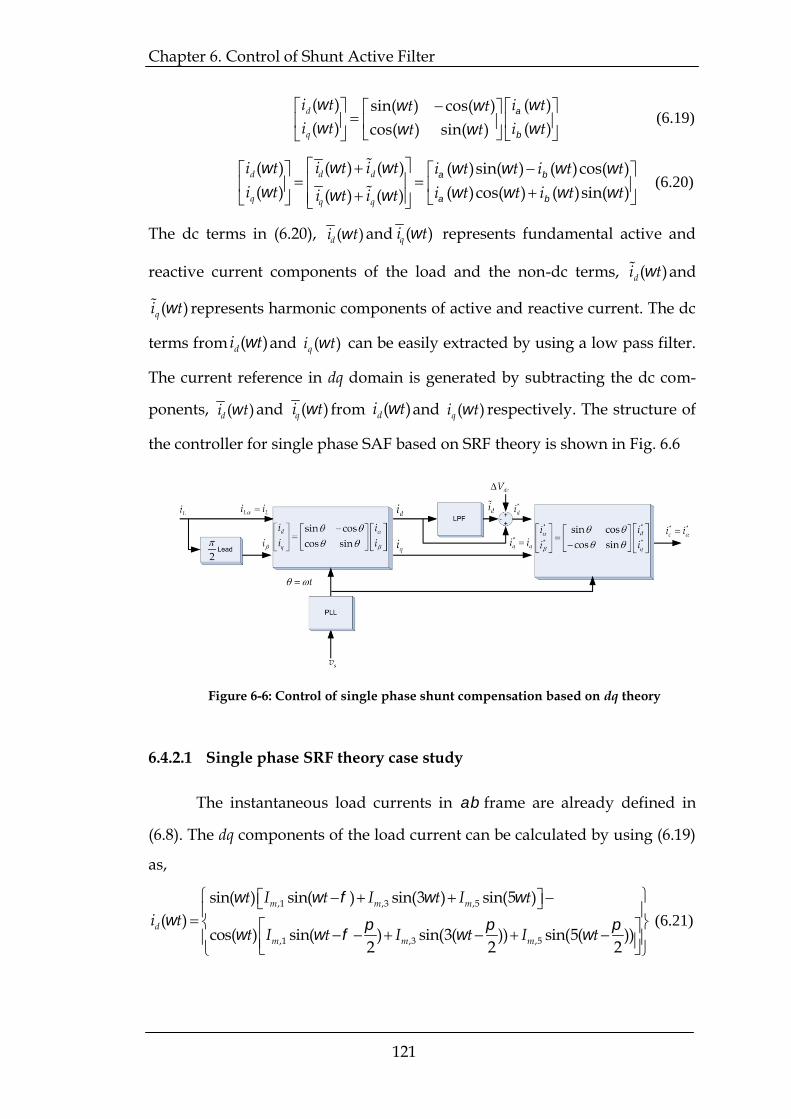
ponents, ( )di t and ( )qi t from ( )di t and ( )qi t respectively. The structure of
the controller for single phase SAF based on SRF theory is shown in Fig. 6.6
6.4.2.1 Single phase SRF theory case study
The instantaneous load currents in frame are already defined in
(6.8). The dq components of the load current can be calculated by using (6.19)
as,
,1 ,3 ,5
,1 ,3 ,5
sin( ) sin( ) sin(3 ) sin(5 )( )
cos( ) sin( ) sin(3( )) sin(5( ))2 2 2
m m m
dm m m
t I t I t I ti t
t I t I t I t
(6.21)
Figure 6-6: Control of single phase shunt compensation based on dq theory
Chapter 6. Control of Shunt Active Filter
122
Solving further,
,1 ,3 ,5
,1 ,3 ,5
sin( ) sin( ) sin(3 ) sin(5 )( )
cos( ) cos( ) cos(3 ) cos(5 )m m m
dm m m
t I t I t I ti t
t I t I t I t
(6.22)
Similarly,
,1 ,3 ,5
,1 ,3 ,5
cos( ) sin( ) sin(3 ) sin(5 )( )
sin( ) cos( ) cos(3 ) cos(5 )m m m
qm m m
t I t I t I ti t
t I t I t I t
(6.23)
Applying trigonometric identities,
,1 ,5 ,3( ) cos( ) ( )cos(4 )d m m mi t I I I t (6.24)
,1 ,3 ,5( ) sin( ) ( )sin(4 )q m m mi t I I I t (6.25)
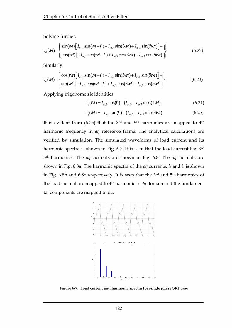
It is evident from (6.25) that the 3rd and 5th harmonics are mapped to 4th
harmonic frequency in dq reference frame. The analytical calculations are
verified by simulation. The simulated waveforms of load current and its
harmonic spectra is shown in Fig. 6.7. It is seen that the load current has 3rd
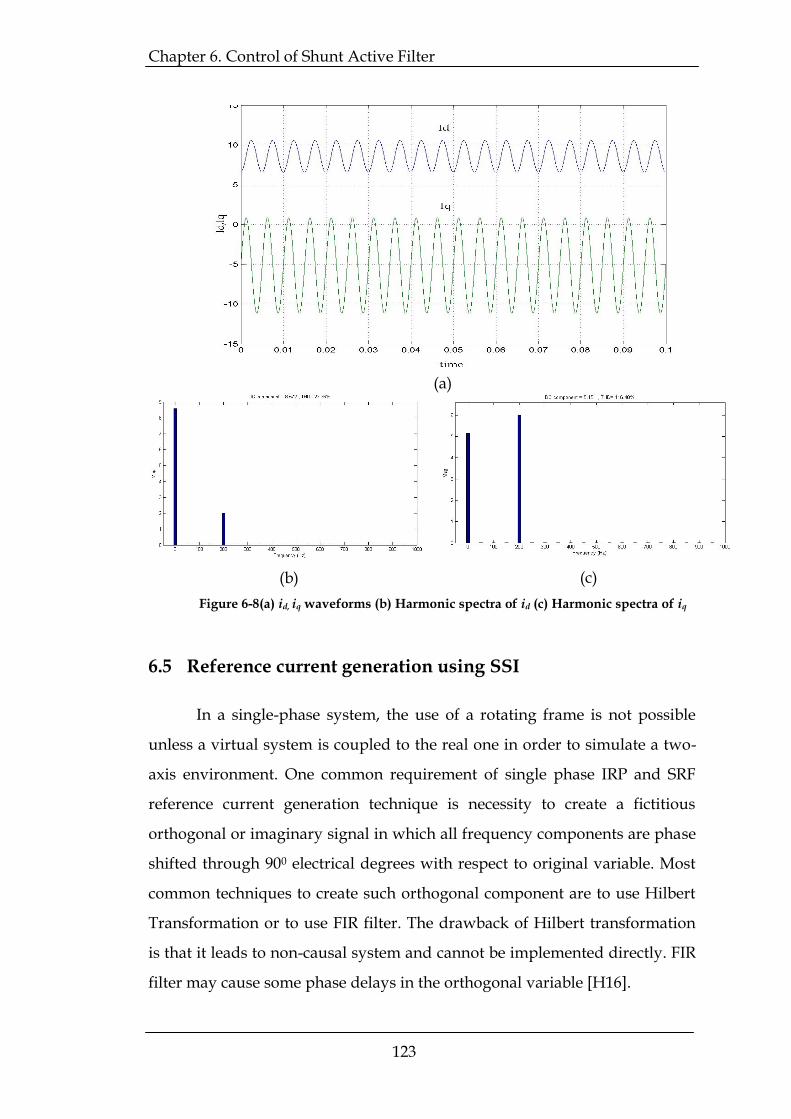
5th harmonics. The dq currents are shown in Fig. 6.8. The dq currents are
shown in Fig. 6.8a. The harmonic spectra of the dq currents, id and iq is shown
in Fig. 6.8b and 6.8c respectively. It is seen that the 3rd and 5th harmonics of
the load current are mapped to 4th harmonic in dq domain and the fundamen-
tal components are mapped to dc.
Figure 6-7: Load current and harmonic spectra for single phase SRF case
Chapter 6. Control of Shunt Active Filter
122
Solving further,
,1 ,3 ,5
,1 ,3 ,5
sin( ) sin( ) sin(3 ) sin(5 )( )
cos( ) cos( ) cos(3 ) cos(5 )m m m
dm m m
t I t I t I ti t
t I t I t I t
(6.22)
Similarly,
,1 ,3 ,5
,1 ,3 ,5
cos( ) sin( ) sin(3 ) sin(5 )( )
sin( ) cos( ) cos(3 ) cos(5 )m m m
qm m m
t I t I t I ti t
t I t I t I t
(6.23)
Applying trigonometric identities,
,1 ,5 ,3( ) cos( ) ( )cos(4 )d m m mi t I I I t (6.24)
,1 ,3 ,5( ) sin( ) ( )sin(4 )q m m mi t I I I t (6.25)
It is evident from (6.25) that the 3rd and 5th harmonics are mapped to 4th
harmonic frequency in dq reference frame. The analytical calculations are
verified by simulation. The simulated waveforms of load current and its
harmonic spectra is shown in Fig. 6.7. It is seen that the load current has 3rd
5th harmonics. The dq currents are shown in Fig. 6.8. The dq currents are
shown in Fig. 6.8a. The harmonic spectra of the dq currents, id and iq is shown
in Fig. 6.8b and 6.8c respectively. It is seen that the 3rd and 5th harmonics of
the load current are mapped to 4th harmonic in dq domain and the fundamen-
tal components are mapped to dc.
Figure 6-7: Load current and harmonic spectra for single phase SRF case
Chapter 6. Control of Shunt Active Filter
123
6.5 Reference current generation using SSI
In a single-phase system, the use of a rotating frame is not possible
unless a virtual system is coupled to the real one in order to simulate a two-
axis environment. One common requirement of single phase IRP and SRF
reference current generation technique is necessity to create a fictitious
orthogonal or imaginary signal in which all frequency components are phase
shifted through 900 electrical degrees with respect to original variable. Most
common techniques to create such orthogonal component are to use Hilbert
Transformation or to use FIR filter. The drawback of Hilbert transformation
is that it leads to non-causal system and cannot be implemented directly. FIR
filter may cause some phase delays in the orthogonal variable [H16].
(a)
(b) (c)Figure 6-8(a) id, iq waveforms (b) Harmonic spectra of id (c) Harmonic spectra of iq
Chapter 6. Control of Shunt Active Filter
124
Alternatively, computation of the SAF reference current can be performed
using Sine Signal Integrator (SSI) with less computational burden. This
approach enables delay less orthogonal signal generation. Moreover, refer-
ence current generation is insensitive to grid voltage distortion. The transfer
function of the basic Second Order Generalized Integrator(SOGI) is defined
by (6.26) which correspond to the block diagram depicted in Fig. 6.9. It
presents two poles located at 0s jw and a zero at 0s .
2 20
( )SOGIsG s
s w
(6.26)
Taking into account Laplace transform of a sine and cosine signal are:
sine 2 20
sG (s)s w
(6.27)
0cosine 2 2
0
G (s)s
(6.28)
Figure 6-9: Block diagram of SOGI
Figure 6-10: Bode Diagram of the basic SOGI
Chapter 6. Control of Shunt Active Filter
125
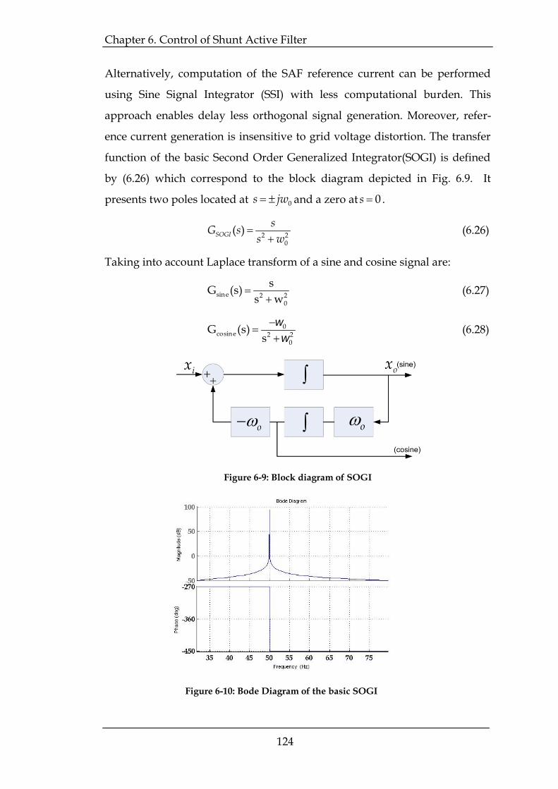
Bode diagram of the continuous time domain transfer function of the SOGI
tuned to 0 2 50rad/sec is shown in Fig. 6.10. Its phase diagram
represents zero phase at 0 and theoretically infinite gain at that frequen-
cy. In rest of the frequencies, the phase takes the values from to2 2 rad.
One of the main characteristics of SOGI is that it presents very narrow band-
width around the resonant frequency, 0 i.e. it is very selective. It also rejects
the dc component, since it has a zero at s=0, thus it shown infinite attenuation
at 0 . The basic SOGI has the disadvantage of having infinite gain at
resonant frequency, which can make the system unstable. To avoid stability
problems associated with the infinite gain and to increase bandwidth, a
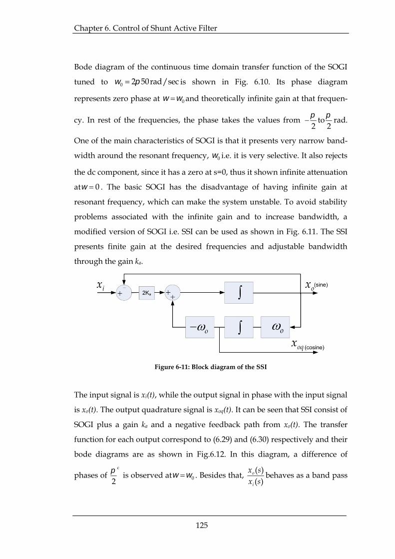
modified version of SOGI i.e. SSI can be used as shown in Fig. 6.11. The SSI
presents finite gain at the desired frequencies and adjustable bandwidth
through the gain ka.
Figure 6-11: Block diagram of the SSI
The input signal is xi(t), while the output signal in phase with the input signal
is xo(t). The output quadrature signal is xoq(t). It can be seen that SSI consist of
SOGI plus a gain ka and a negative feedback path from xo(t). The transfer
function for each output correspond to (6.29) and (6.30) respectively and their
bode diagrams are as shown in Fig.6.12. In this diagram, a difference of
phases of c
2is observed at 0 . Besides that, ( )
( )o
i
x sx s
behaves as a band pass
Chapter 6. Control of Shunt Active Filter
126
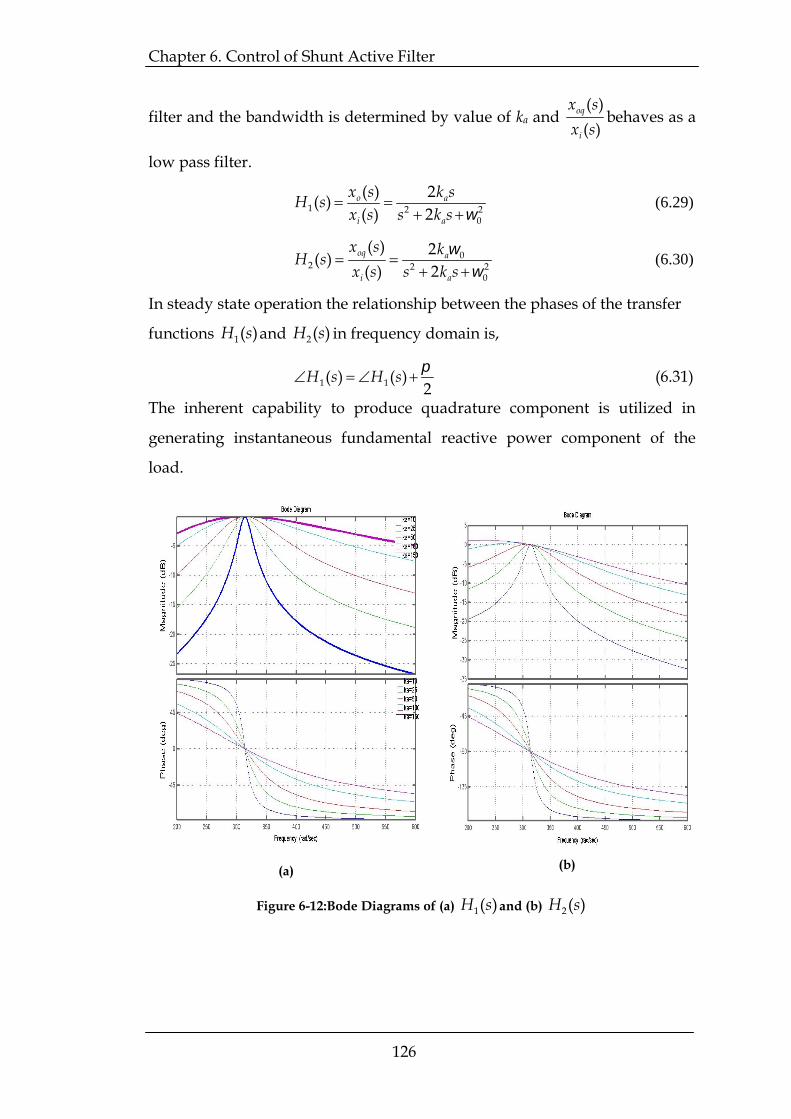
filter and the bandwidth is determined by value of ka and( )( )
oq
i
x sx s
behaves as a
low pass filter.
1 2 20
( ) 2( )( ) 2
o a
i a
x s k sH sx s s k s
(6.29)
02 2 2
0
( ) 2( )( ) 2
oq a
i a
x s kH sx s s k s
(6.30)
In steady state operation the relationship between the phases of the transfer
functions H s1( )and H s2( ) in frequency domain is,
H s H s1 1( ) ( )2
(6.31)
The inherent capability to produce quadrature component is utilized in
generating instantaneous fundamental reactive power component of the
load.
(a) (b)
Figure 6-12:Bode Diagrams of (a) H s1( )and (b) H s2( )

Chapter 6. Control of Shunt Active Filter
127
6.6 Reference current generation for direct control of SAF
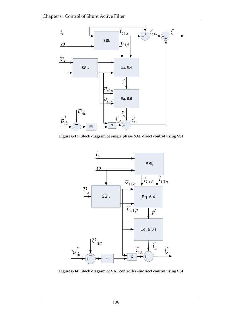
The block diagram for SAF reference current generation based on SSI
is depicted in Fig. 6.13. There are two SSI blocks to extract fundamental
components of supply voltage and load current respectively. The SSIv block
generates sv 1 and sv 1 components of the supply voltage sv . As the SSIv and
SSII blocks are sharply tuned to fundamental frequency, sv 1 and sv 1 outputs
are insensitive to distortion present in sv .The harmonic component of the
load current L hi*1 is calculated by subtracting component of load current
Li 1 from the actual load current Li . The output of the SSII block is the
fundamental component of the load current (including active and reactive
components). To extract the fundamental reactive current, single phase IRP
theory as discussed in section 6.4.1 has been used. The instantaneous reactive
power reference q* can be calculated by using (6.4). Equating real power to
zero, the fundamental reactive current reference can be calculated using (6.6).
The resulting equation reactive current reference is,
v t v ti tv t v t q ti t v t v t
*
* 2 2
( ) ( ) 0( ) 1( ) ( ) ( )( ) ( ) ( )
(6.32)
In (6.32), the reactive power component is fundamental i.e. q t( ) as the
calculation of q(wt) performed on fundamental terms. The resulting
expression for i t* ( ) becomes
s s L s Lv v t i t v t i ti t
v t v t1 1 1 1 1*
2 2
( ) ( ) ( ) ( )( )
( ) ( )
(6.33)
As the system is single phase, i* component can be neglected and the i*
component acts as the reactive current reference. The necessary fundamental
active current, dci*1 needed to be absorbed by the SAF to maintain dc bus
voltage is generated by a DC voltage controller and added to i* . The resulting
fundamental current i *1 and L hi*
1 are added to generate the SAF reference
current ci* .
Chapter 6. Control of Shunt Active Filter
128
6.7 Reference current generation for indirect control of SAF
In indirect control of SAF, the supply current is sensed and the SAF
switches are controlled in such a manner so that the supply current is sinu-
soidal and in phase with the supply voltage. A This means the SAF current is
indirectly controlled. As the sensed current is sinusoidal at fundamental
frequency, this offers an advantage of selecting a low bandwidth current
transducer. Ideally, the supply should generate only fundamental active
component of the load current. In attempt to maintain sinusoidal and in
phase supply current, the SAF indirectly supplies the fundamental reactive
and harmonic current. The block diagram of the SAF reference current
extraction for indirect control is shown in Fig. 6.14. The SSI structure is as
same as shown for direct current control technique. As both of the SSI units
extract fundamental components of supply voltage and load current
respectively, the instantaneous fundamental active power p t( ) can be
calculated by using (6.4). The component i *1 can be calculated as,
v t v t i t v t i ti t
v t v t1 1 1 1 1*
2 2
( ) ( ) ( ) ( ) ( )( )
( ) ( )
(6.34)
The desired supply current is addition of i t* ( ) and dci*1 . The use of SSI
eliminates the need of additional low pass filter to extract fundamental
powers and a2 lag/lead for supply voltage and load current signals to
generate fictitious signal to apply IRP theory as proposed by [H15]. The
resultant structure of the SAF controller is greatly simplified and eliminates
the need of phase lag elements and filters.
Chapter 6. Control of Shunt Active Filter
129
Figure 6-13: Block diagram of single phase SAF direct control using SSI
Figure 6-14: Block diagram of SAF controller -indirect control using SSI
Chapter 6. Control of Shunt Active Filter
130
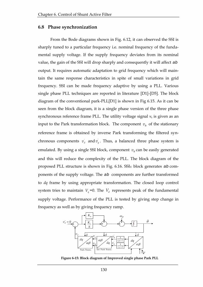
6.8 Phase synchronization
From the Bode diagrams shown in Fig. 6.12, it can observed the SSI is
sharply tuned to a particular frequency i.e. nominal frequency of the funda-
mental supply voltage. If the supply frequency deviates from its nominal
value, the gain of the SSI will drop sharply and consequently it will affect
output. It requires automatic adaptation to grid frequency which will main-
tain the same response characteristics in spite of small variations in grid
frequency. SSI can be made frequency adaptive by using a PLL. Various
single phase PLL techniques are reported in literature [D1]-[D5]. The block
diagram of the conventional park-PLL[D1] is shown in Fig 6.15. As it can be
seen from the block diagram, it is a single phase version of the three phase
synchronous reference frame PLL. The utility voltage signal vs is given as an
input to the Park transformation block. The component v of the stationary
reference frame is obtained by inverse Park transforming the filtered syn-
chronous components 'dv and '
qv . Thus, a balanced three phase system is
emulated. By using a single SSI block, component v can be easily generated
and this will reduce the complexity of the PLL. The block diagram of the
proposed PLL structure is shown in Fig. 6.16. SSIV block generates com-
ponents of the supply voltage. The components are further transformed
to dq frame by using appropriate transformation. The closed loop control
system tries to maintain qV =0. The dV represents peak of the fundamental
supply voltage. Performance of the PLL is tested by giving step change in
frequency as well as by giving frequency ramp.
Figure 6-15: Block diagram of Improved single phase Park PLL

Chapter 6. Control of Shunt Active Filter
131
Dynamic performance of the PLL is tested by giving step input of input
frequency as shown in Fig. 6.17. The performance of the PLL under distorted
utility conditions is shown in Fig. 6.18. From the responses, it can be con-
cluded that the SSI based PLL has satisfactory dynamic response and has
ability to extract instantaneous phase angle information even in presence of
distorted supply.
Figure 6-18: Frequency tracking performance of PLL
Figure 6-16: Block diagram of single phase PLL based on SSI
Figure 6-17: PLL performance under distorted supply voltage conditions
Chapter 6. Control of Shunt Active Filter
132
6.9 SAF current control
The generated SAF reference current is sent to the current controller.
The current controller takes the instantaneous feedback of the SAF current at
its input ( ci ) and the reference current ( ci* ) and then creates the switching
signals to the individual switches of VSI for regulation of SAF current. Per-
formance of current controller can be characterized by following
requirements [G8]:
Non sinusoidal multi frequency tracking.
Ability to operate with low VSI output inductance (Lac < 5%).
High di/dt reference current tracking and high current control-
ler. bandwidth for tracking of high frequency harmonics.
Minimization of low as well as high frequency errors in current.
Desired implementation by constant switching frequency PWM
scheme.
Maintain predictable ripple bounds.
Different current control strategies are reported in literature for SAF
applications. Hysteresis and sliding mode controls allow both a direct control
of the current but at the price of a time-varying switching frequency. Hyste-
resis current regulators are on-off type current regulators and widely utilized
for tracking of non-sinusoidal, multiple frequency and high di/dt current
references. When analog implementation is utilized, hysteresis current
regulators exhibit high bandwidth and superior tracking capability of the
reference currents with high di/dt. Various techniques to implement hystere-
sis control are discussed in [I2]-[I7]. The well known drawback of hysteresis
control technique is variable switching frequency. Hysteresis current regula-
tors also generate an undesirable ‘white noise’ current spectrum as a result of
variable inverter switching frequency. The design of the output filter is also
difficult for these methods as well as control of noise level. [G8].
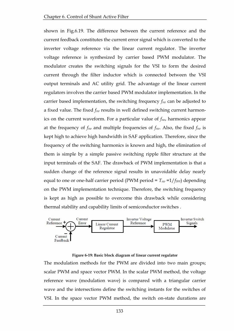
Linear and on-off current controllers also form a viable solution for
SAF applications. The basic principle of the linear current regulators is
Chapter 6. Control of Shunt Active Filter
133
shown in Fig.6.19. The difference between the current reference and the
current feedback constitutes the current error signal which is converted to the
inverter voltage reference via the linear current regulator. The inverter
voltage reference is synthesized by carrier based PWM modulator. The
modulator creates the switching signals for the VSI to form the desired
current through the filter inductor which is connected between the VSI
output terminals and AC utility grid. The advantage of the linear current
regulators involves the carrier based PWM modulator implementation. In the
carrier based implementation, the switching frequency fsw can be adjusted to
a fixed value. The fixed fsw results in well defined switching current harmon-
ics on the current waveform. For a particular value of fsw, harmonics appear
at the frequency of fsw and multiple frequencies of fsw. Also, the fixed fsw is
kept high to achieve high bandwidth in SAF application. Therefore, since the
frequency of the switching harmonics is known and high, the elimination of
them is simple by a simple passive switching ripple filter structure at the
input terminals of the SAF. The drawback of PWM implementation is that a
sudden change of the reference signal results in unavoidable delay nearly
equal to one or one-half carrier period (PWM period = Tsw =1/fSW) depending
on the PWM implementation technique. Therefore, the switching frequency
is kept as high as possible to overcome this drawback while considering
thermal stability and capability limits of semiconductor switches .
Figure 6-19: Basic block diagram of linear current regulator
The modulation methods for the PWM are divided into two main groups;
scalar PWM and space vector PWM. In the scalar PWM method, the voltage
reference wave (modulation wave) is compared with a triangular carrier
wave and the intersections define the switching instants for the switches of
VSI. In the space vector PWM method, the switch on-state durations are
Chapter 6. Control of Shunt Active Filter
134
calculated from the complex number from volt-seconds balance equation for
the inverter voltage and the switch pulse pattern is programmed via digital
PWM.
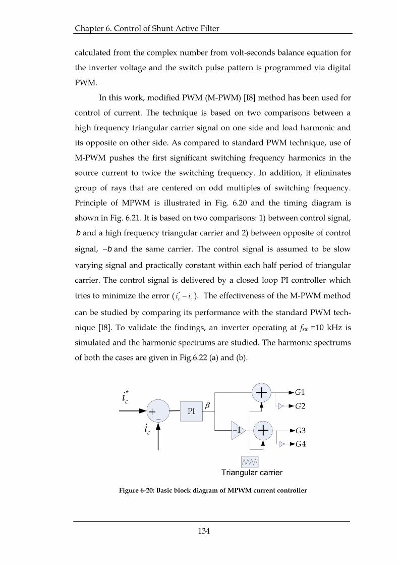
In this work, modified PWM (M-PWM) [I8] method has been used for
control of current. The technique is based on two comparisons between a
high frequency triangular carrier signal on one side and load harmonic and
its opposite on other side. As compared to standard PWM technique, use of
M-PWM pushes the first significant switching frequency harmonics in the
source current to twice the switching frequency. In addition, it eliminates
group of rays that are centered on odd multiples of switching frequency.
Principle of MPWM is illustrated in Fig. 6.20 and the timing diagram is
shown in Fig. 6.21. It is based on two comparisons: 1) between control signal,
and a high frequency triangular carrier and 2) between opposite of control
signal, and the same carrier. The control signal is assumed to be slow
varying signal and practically constant within each half period of triangular
carrier. The control signal is delivered by a closed loop PI controller which
tries to minimize the error ( c ci i* ). The effectiveness of the M-PWM method
can be studied by comparing its performance with the standard PWM tech-
nique [I8]. To validate the findings, an inverter operating at fsw =10 kHz is
simulated and the harmonic spectrums are studied. The harmonic spectrums
of both the cases are given in Fig.6.22 (a) and (b).
Figure 6-20: Basic block diagram of MPWM current controller

Chapter 6. Control of Shunt Active Filter
135
Figure 6-21: Timing diagram of MPWM current control technique
(a)
Chapter 6. Control of Shunt Active Filter
136
(b)
Figure 6-22: Comparison of vc spectrum: a) with S-PWM b) with M-PWM
6.10 Switching ripple filter for the SAF
The current ripple generated by the VSI of the SAF power circuitry can
spread to the power line through the PCC where the PAF system is con-
nected to the power system. High frequency switching harmonics create
noise problems for other loads connected to the same PCC. To filter the high
frequency switching ripple currents due to the switching of the VSI, passive
switching ripple filters are placed at the PCC as an integral part of the SAF.
Linear current regulators generate regular PWM ripples around the switch-
ing frequency and its multiples and sidebands over the frequency spectrum.
The M-PWM switching technique causes the switching ripple to be at 2fsw as
shown in the previous discussed above. This section presents overview of
different switching ripple filter topologies and design of broad band switch-
ing ripple filter topology to reduce switching ripples.
6.10.1 Switching Ripple Filter Topologies
The choice of SRF topology is directly related to the ripple currents
frequency spectrum, hence that is related to the current regulator type uti-
lized in the PAF control system. The switching ripple currents of linear
current regulators are observed at switching frequency (fsw) and its multiples
(2fsw, 3fsw...) i.e. at specific frequency components which depend upon the
switching frequency. Therefore, a tuned type switching ripple filter which is
Chapter 6. Control of Shunt Active Filter
137
tuned to fsw should be utilized to filter the switching ripple currents of the
PAF when utilizing linear current regulators. Various filter topologies are
already shown in Fig. 3.4 of Chapter 3. Broad band tuned filter is the most
suitable choice considering the specific harmonic frequencies present in the
current.
6.10.2 Broad-band Tuned Type switching ripple filter
The broad-band tuned type switching ripple filter (RF) illustrated in
Figure 3.4.b is utilized to filter the switching ripple currents created by the
linear current regulators in the SAF applications and also for providing
passive damping of the parallel resonance for a wide frequency range [F7].
The filter involves two separate paths; one for the attenuation of the switch-
ing ripple currents and the other for damping of the load and/or source side
induced resonances. The LF, CF branch is a series resonant branch which is
tuned to frequency fsw. The impedances of CF and LF cancel each other at fsw
and the total impedance of filter is equal to filter resistance RF at fsw. To sink
the switching ripple currents, RF should be low. RF is mainly constituted by
the internal resistance of LF. By tuning resonant frequency of the LF CF RF
filter to fsw, the most dominant switching ripple currents at fsw are filtered
through the low impedance path. The value of the filter damping resistor Rd
is selected such that it will damp out the resonances for a wide frequency
range with the capacitor C connected in series with the two parallel con-
nected arms. The series resonant frequency fs of the broad-band tuned type
filter, considering the inclusion of C to the filter structure, is defined as,
sF
FF
fC CL
C C
1
2
(6.35)
For the design simplicity, the approximate value of fs can be expressed in
terms of LF and CF values, as,
Chapter 6. Control of Shunt Active Filter
138
sF F
fL C1
2 (6.36)
The size of C should be such that, C >> CF. As suggested in [F5], the value of
CF should be such that,
FC C10 (6.37)
However, the larger C sizes are not preferred since they result in excessive
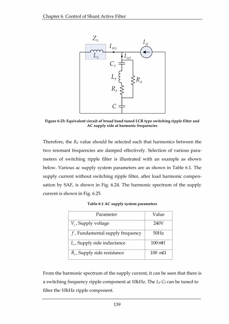
reactive power at the fundamental frequency. The equivalent circuit of broad
band switching ripple filter at harmonic frequencies is shown in Fig. 6.23.
The transfer function T(s) defined as the ratio of the line current IHS to har-
monic current source IH expressed in terms of filter circuit components CF, LF,
C, and Rd as follows,
F F d F F F d
S F F F S F d F F S F d
s L C CR s L C s C C RT ss L L C C s L L C CR s L C L C s C C R
3 2
4 3 2
( ) 1( )( ) ( ) ( ) ( ) 1
(6.38)
It can be seen that, very low value of Rd there can exist a condition for paral-
lel resonance between switching ripple filter capacitance C and supply side
inductance Ls, at frequency fp1,
ps
fL C1
12 (6.39)
As Rd increases, there is a chance of parallel resonance which occurs between
filter capacitor CF, filter inductor LF and line inductance LS at a frequency fp2
given as,
ps F F
fL L C2
12 ( )
(6.40)
Chapter 6. Control of Shunt Active Filter
139
Therefore, the Rd value should be selected such that harmonics between the
two resonant frequencies are damped effectively. Selection of various para-
meters of switching ripple filter is illustrated with an example as shown
below. Various ac supply system parameters are as shown in Table 6.1. The
supply current without switching ripple filter, after load harmonic compen-
sation by SAF, is shown in Fig. 6.24. The harmonic spectrum of the supply
current is shown in Fig. 6.25.
Table 6-1 AC supply system parameters
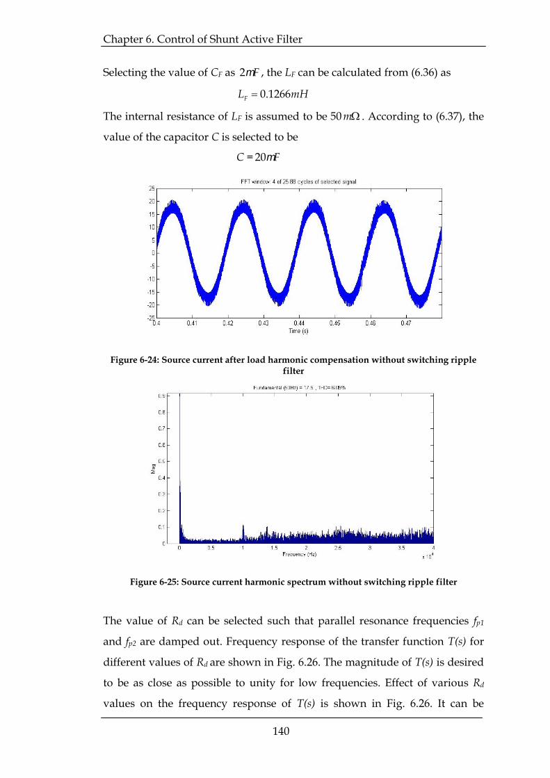
From the harmonic spectrum of the supply current, it can be seen that there is
a switching frequency ripple component at 10kHz. The LF CF can be tuned to
filter the 10kHz ripple component.
Figure 6-23: Equivalent circuit of broad band tuned LCR type switching ripple filter andAC supply side at harmonic frequencies
Parameter Value
sV , Supply voltage 240V
f , Fundamental supply frequency 50Hz
sL , Supply side inductance 100 H
sR , Supply side resistance 100 m
Chapter 6. Control of Shunt Active Filter
140
Selecting the value of CF as F2 , the LF can be calculated from (6.36) as
FL mH0.1266
The internal resistance of LF is assumed to be 50 m . According to (6.37), the
value of the capacitor C is selected to be
C = F20
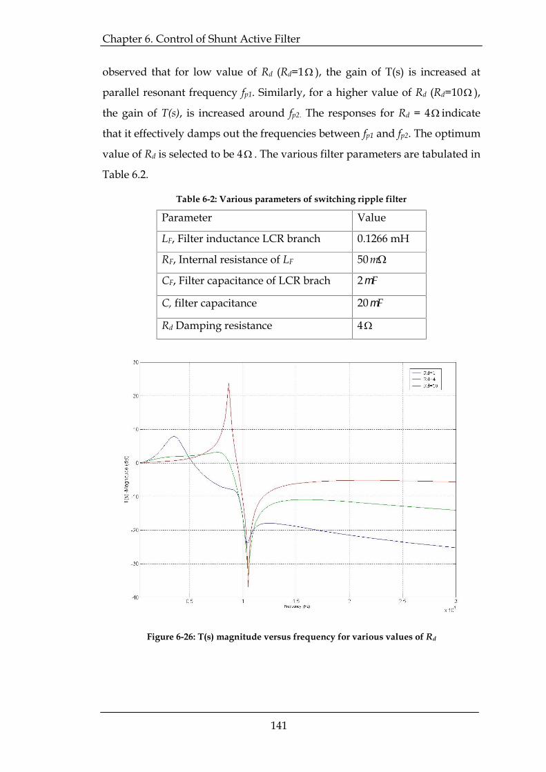
The value of Rd can be selected such that parallel resonance frequencies fp1
and fp2 are damped out. Frequency response of the transfer function T(s) for
different values of Rd are shown in Fig. 6.26. The magnitude of T(s) is desired
to be as close as possible to unity for low frequencies. Effect of various Rd
values on the frequency response of T(s) is shown in Fig. 6.26. It can be
Figure 6-24: Source current after load harmonic compensation without switching ripplefilter
Figure 6-25: Source current harmonic spectrum without switching ripple filter
Chapter 6. Control of Shunt Active Filter
141
observed that for low value of Rd (Rd=1 ), the gain of T(s) is increased at
parallel resonant frequency fp1. Similarly, for a higher value of Rd (Rd=10 ),
the gain of T(s), is increased around fp2. The responses for Rd = 4 indicate
that it effectively damps out the frequencies between fp1 and fp2. The optimum
value of Rd is selected to be 4 . The various filter parameters are tabulated in
Table 6.2.
Table 6-2: Various parameters of switching ripple filter
Parameter Value
LF, Filter inductance LCR branch 0.1266 mH
RF, Internal resistance of LF 50 m
CF, Filter capacitance of LCR brach 2 F
C, filter capacitance 20 F
Rd Damping resistance 4
Figure 6-26: T(s) magnitude versus frequency for various values of Rd
Chapter 6. Control of Shunt Active Filter
142
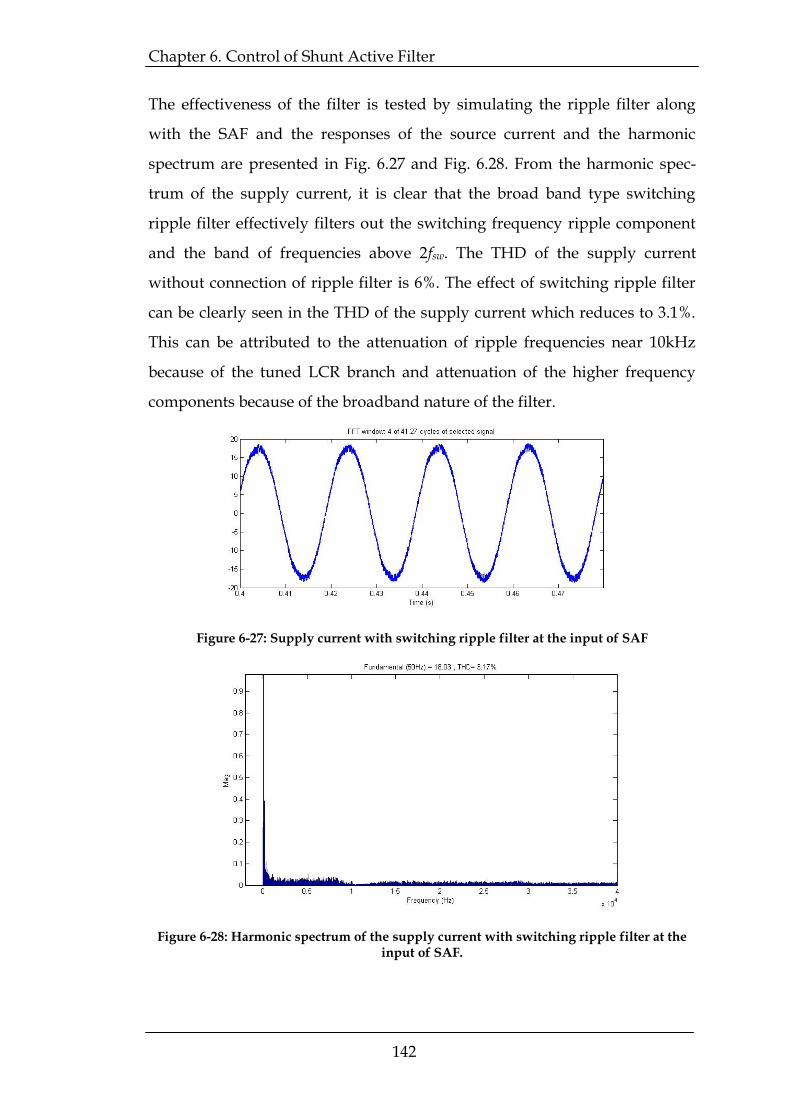
The effectiveness of the filter is tested by simulating the ripple filter along
with the SAF and the responses of the source current and the harmonic
spectrum are presented in Fig. 6.27 and Fig. 6.28. From the harmonic spec-
trum of the supply current, it is clear that the broad band type switching
ripple filter effectively filters out the switching frequency ripple component
and the band of frequencies above 2fsw. The THD of the supply current
without connection of ripple filter is 6%. The effect of switching ripple filter
can be clearly seen in the THD of the supply current which reduces to 3.1%.
This can be attributed to the attenuation of ripple frequencies near 10kHz
because of the tuned LCR branch and attenuation of the higher frequency
components because of the broadband nature of the filter.
Figure 6-27: Supply current with switching ripple filter at the input of SAF
Figure 6-28: Harmonic spectrum of the supply current with switching ripple filter at theinput of SAF.

Chapter 6. Control of Shunt Active Filter
143
6.11 Summary
In this chapter, a method based on SSI to extract reference current of
single phase SAF is presented. Two models to extract SAF reference current
for direct and indirect controlled SAFs have been put forth. A single phase
PLL based on SSI is also proposed. The current controller is based on M-
PWM technique. The design of broad-band tuned LCR filter to minimize
switching frequency ripple is also discussed along with its simulation results.