CHAPTER 6 APPLICATION OF NUMERICAL …homes.civil.aau.dk/.../Bennetsen_JC/chap6_del_5.pdfCHAPTER 6 APPLICATION OF NUMERICAL SIMULATION TO VENTILATED FLOW PROBLEMS 1) Personal communication

CHAPTER 6 APPLICATION OF NUMERICAL SIMULATION TO VENTILATED FLOW PROBLEMS

101


168

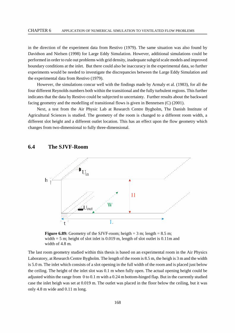
Figure 6.89: Geometry of the SJVF-room; heigth = 3 m; length = 8.5 m;width = 5 m; height of slot inlet is 0.019 m, length of slot outlet is 0.11m and width of 4.8 m.

in the direction of the experiment data from Restivo (1979). The same situation was also found byDavidson and Nielsen (1998) for Large Eddy Simulation. However, additional simulations could beperformed in order to rule out problems with grid density, inadequate subgrid scale models and improvedboundary conditions at the inlet. But there could also be inaccuracy in the experimental data, so furtherexperiments would be needed to investigate the discrepancies between the Large Eddy Simulation andthe experimental data from Restivo (1979).

However, the simulations concur well with the findings made by Armaly et al. (1983), for all thefour different Reynolds numbers both within the transitional and the fully turbulent regions. This furtherindicates that the data by Restivo could be subjected to uncertainty. Further results about the backwardfacing geometry and the modelling of transitional flows is given in Bennetsen (C) (2001).

Next, a test from the Air Physic Lab at Research Centre Bygholm, The Danish Institute ofAgricultural Sciences is studied. The geometry of the room is changed to a different room width, adifferent slot height and a different outlet location. This has an effect upon the flow geometry whichchanges from two-dimensional to fully three-dimensional.

6.4 The SJVF-Room

The last room geometry studied within this thesis is based on an experimental room in the Air PhysicsLaboratory, at Research Centre Bygholm. The length of the room is 8.5 m, the heigh is 3 m and the widthis 5.0 m. The inlet which consists of a slot opening in the full width of the room and is placed just belowthe ceiling. The height of the inlet slot was 0.1 m when fully open. The actual opening height could beadjusted within the range from 0 to 0.1 m with a 0.24 m bottom-hinged flap. But in the currently studiedcase the inlet heigh was set at 0.019 m. The outlet was placed in the floor below the ceiling, but it wasonly 4.8 m wide and 0.11 m long.


169

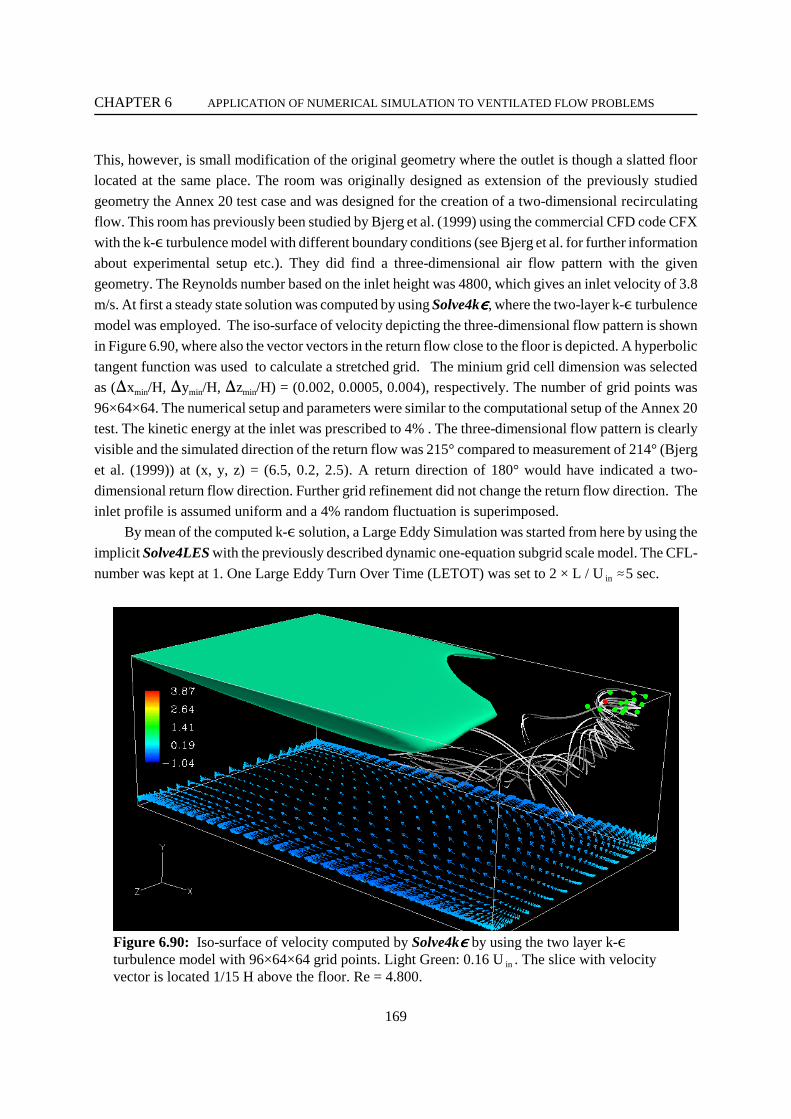
Figure 6.90: Iso-surface of velocity computed by Solve4kIIII by using the two layer k-Iturbulence model with 96×64×64 grid points. Light Green: 0.16 U in . The slice with velocityvector is located 1/15 H above the floor. Re = 4.800.

This, however, is small modification of the original geometry where the outlet is though a slatted floorlocated at the same place. The room was originally designed as extension of the previously studiedgeometry the Annex 20 test case and was designed for the creation of a two-dimensional recirculatingflow. This room has previously been studied by Bjerg et al. (1999) using the commercial CFD code CFXwith the k-I turbulence model with different boundary conditions (see Bjerg et al. for further informationabout experimental setup etc.). They did find a three-dimensional air flow pattern with the givengeometry. The Reynolds number based on the inlet height was 4800, which gives an inlet velocity of 3.8m/s. At first a steady state solution was computed by using Solve4kIIII, where the two-layer k-I turbulencemodel was employed. The iso-surface of velocity depicting the three-dimensional flow pattern is shownin Figure 6.90, where also the vector vectors in the return flow close to the floor is depicted. A hyperbolictangent function was used to calculate a stretched grid. The minium grid cell dimension was selectedas (Fxmin/H, Fymin/H, Fzmin/H) = (0.002, 0.0005, 0.004), respectively. The number of grid points was96×64×64. The numerical setup and parameters were similar to the computational setup of the Annex 20test. The kinetic energy at the inlet was prescribed to 4% . The three-dimensional flow pattern is clearlyvisible and the simulated direction of the return flow was 215° compared to measurement of 214° (Bjerget al. (1999)) at (x, y, z) = (6.5, 0.2, 2.5). A return direction of 180° would have indicated a two-dimensional return flow direction. Further grid refinement did not change the return flow direction. Theinlet profile is assumed uniform and a 4% random fluctuation is superimposed.

By mean of the computed k-I solution, a Large Eddy Simulation was started from here by using theimplicit Solve4LES with the previously described dynamic one-equation subgrid scale model. The CFL-number was kept at 1. One Large Eddy Turn Over Time (LETOT) was set to 2 × L / U in Z5 sec.


170

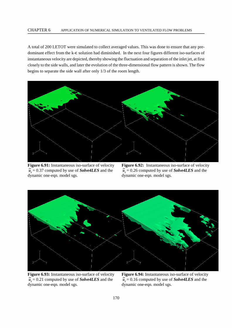
Figure 6.91: Instantaneous iso-surface of velocity= 0.37 computed by use of Solve4LES and the

dynamic one-eqn. model sgs.







A total of 200 LETOT were simulated to collect averaged values. This was done to ensure that any pre-dominant effect from the k-I solution had diminished. In the next four figures different iso-surfaces ofinstantaneous velocity are depicted, thereby showing the fluctuation and separation of the inlet jet, at firstclosely to the side walls, and later the evolution of the three-dimensional flow pattern is shown. The flowbegins to separate the side wall after only 1/3 of the room length.


1) Personal communication with Senior Scientist Guoqiang Zhang, Danish Institute ofAgricultural Sciences, Research Centre Bygholm.

171

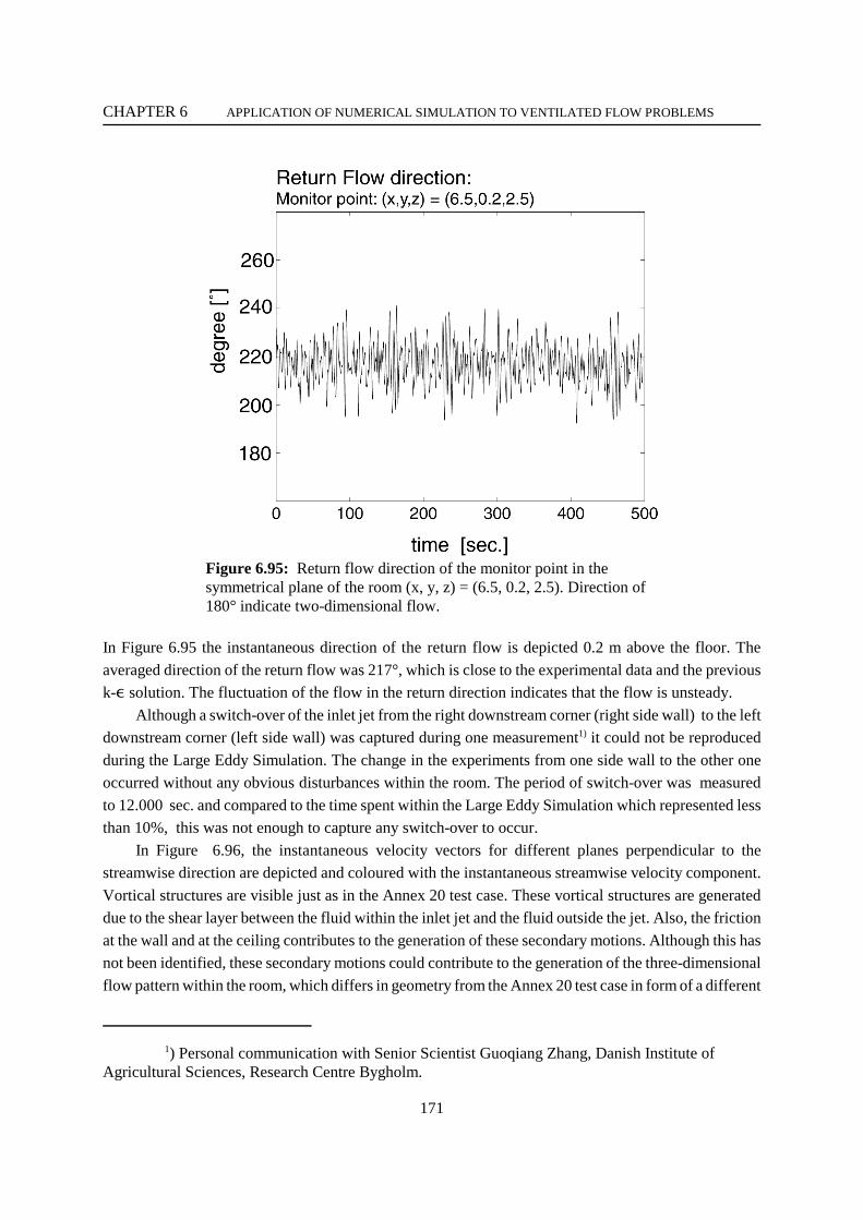
Figure 6.95: Return flow direction of the monitor point in thesymmetrical plane of the room (x, y, z) = (6.5, 0.2, 2.5). Direction of180° indicate two-dimensional flow.

In Figure 6.95 the instantaneous direction of the return flow is depicted 0.2 m above the floor. Theaveraged direction of the return flow was 217°, which is close to the experimental data and the previousk-I solution. The fluctuation of the flow in the return direction indicates that the flow is unsteady.

Although a switch-over of the inlet jet from the right downstream corner (right side wall) to the leftdownstream corner (left side wall) was captured during one measurement1) it could not be reproducedduring the Large Eddy Simulation. The change in the experiments from one side wall to the other oneoccurred without any obvious disturbances within the room. The period of switch-over was measuredto 12.000 sec. and compared to the time spent within the Large Eddy Simulation which represented lessthan 10%, this was not enough to capture any switch-over to occur.

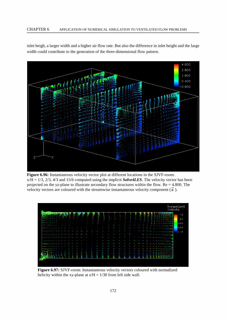
In Figure 6.96, the instantaneous velocity vectors for different planes perpendicular to thestreamwise direction are depicted and coloured with the instantaneous streamwise velocity component.Vortical structures are visible just as in the Annex 20 test case. These vortical structures are generateddue to the shear layer between the fluid within the inlet jet and the fluid outside the jet. Also, the frictionat the wall and at the ceiling contributes to the generation of these secondary motions. Although this hasnot been identified, these secondary motions could contribute to the generation of the three-dimensionalflow pattern within the room, which differs in geometry from the Annex 20 test case in form of a different


172

Figure 6.96: Instantaneous velocity vector plot at different locations in the SJVF-room: x/H = 1/3, 2/3, 4/3 and 15/6 computed using the implicit Solve4LES. The velocity vector has beenprojected on the yz-plane to illustrate secondary flow structures within the flow. Re = 4.800. Thevelocity vectors are coloured with the streamwise instantaneous velocity component ( ).

Figure 6.97: SJVF-room: Instantaneous velocity vectors coloured with normalizedhelicity within the xy-plane at z/H = 1/30 from left side wall.

inlet heigh, a larger width and a higher air flow rate. But also the difference in inlet height and the largewidth could contribute to the generation of the three-dimensional flow pattern.


173

Figure 6.99: SJVF-room: Instantaneous velocity vectors coloured with normalizedhelicity within the xy-plane at z/H = 0.5 (symmetrical plane) from left side wall.

Figure 6.100: SJVF-room: Instantaneous velocity vectors coloured with normalizedhelicity within the xy-plane at z/H = 0.9 from left side wall.

Figure 6.98: SJVF-room: Instantaneous velocity vectors coloured with normalizedhelicity within the xy-plane at z/H = 0.1 from left side wall.

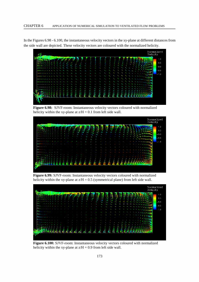
In the Figures 6.98 - 6.100, the instantaneous velocity vectors in the xy-plane at different distances fromthe side wall are depicted. These velocity vectors are coloured with the normalized helicity.


174

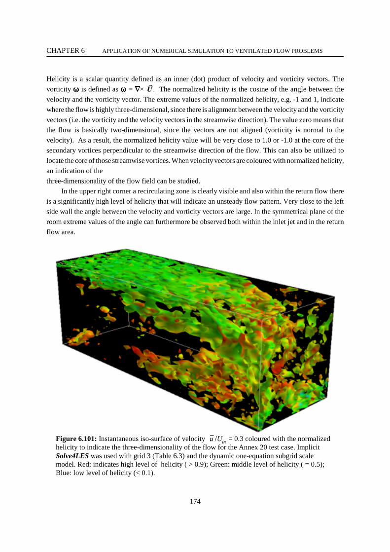
Figure 6.101: Instantaneous iso-surface of velocity = 0.3 coloured with the normalizedhelicity to indicate the three-dimensionality of the flow for the Annex 20 test case. ImplicitSolve4LES was used with grid 3 (Table 6.3) and the dynamic one-equation subgrid scalemodel. Red: indicates high level of helicity ( > 0.9); Green: middle level of helicity ( = 0.5);Blue: low level of helicity (< 0.1).

Helicity is a scalar quantity defined as an inner (dot) product of velocity and vorticity vectors. Thevorticity qqqq is defined as qqqq = iiii× . The normalized helicity is the cosine of the angle between thevelocity and the vorticity vector. The extreme values of the normalized helicity, e.g. -1 and 1, indicatewhere the flow is highly three-dimensional, since there is alignment between the velocity and the vorticityvectors (i.e. the vorticity and the velocity vectors in the streamwise direction). The value zero means thatthe flow is basically two-dimensional, since the vectors are not aligned (vorticity is normal to thevelocity). As a result, the normalized helicity value will be very close to 1.0 or -1.0 at the core of thesecondary vortices perpendicular to the streamwise direction of the flow. This can also be utilized tolocate the core of those streamwise vortices. When velocity vectors are coloured with normalized helicity,an indication of the three-dimensionality of the flow field can be studied.

In the upper right corner a recirculating zone is clearly visible and also within the return flow thereis a significantly high level of helicity that will indicate an unsteady flow pattern. Very close to the leftside wall the angle between the velocity and vorticity vectors are large. In the symmetrical plane of theroom extreme values of the angle can furthermore be observed both within the inlet jet and in the returnflow area.


175

Figure 6.102: Comparison between computedvelocity profile by the two-layer k-I turbulencemodel and the time-averaged velocity from LES byusing the dynamic one-equation sgs model close tothe left side wall. (x/H=1.5; z/H = 1/6). Red: two-layer k-I turbulence mode; Blue: LES withDynamic One-eqn. sgs. Markes: Measurement:Bjerg et al.(1999).

Figure 6.103: Comparison between computedvelocity profile by the two-layer k-I turbulencemodel and the time-averaged velocity from LES byusing the dynamic one-equation sgs model at thesymmetry plane. (x/H=1.5; z/H = 5/6). Red: two-layer k-I turbulence mode; Blue: LES withDynamic One-eqn. sgs. Markes: Measurement:Bjerg et al.(1999).

The level of helicity is compared to the Annex 20 test case depicted in Figure 6.101, which shows theinstantaneous iso-surface of the streamwise velocity, coloured with the absolute value of the normalizedhelicity. For the inlet jet the level of helicity is at a moderate level, and as the back wall is approachedthe level of helicity is increased thus indicating that the flow is becoming more and more three-dimensional and chaotic. The first part of the Annex 20 room also indicates that the flow pattern is almosttwo-dimensional. This was also confirmed by comparing the probability density for points in thesymmetrical plane and close to the side walls.

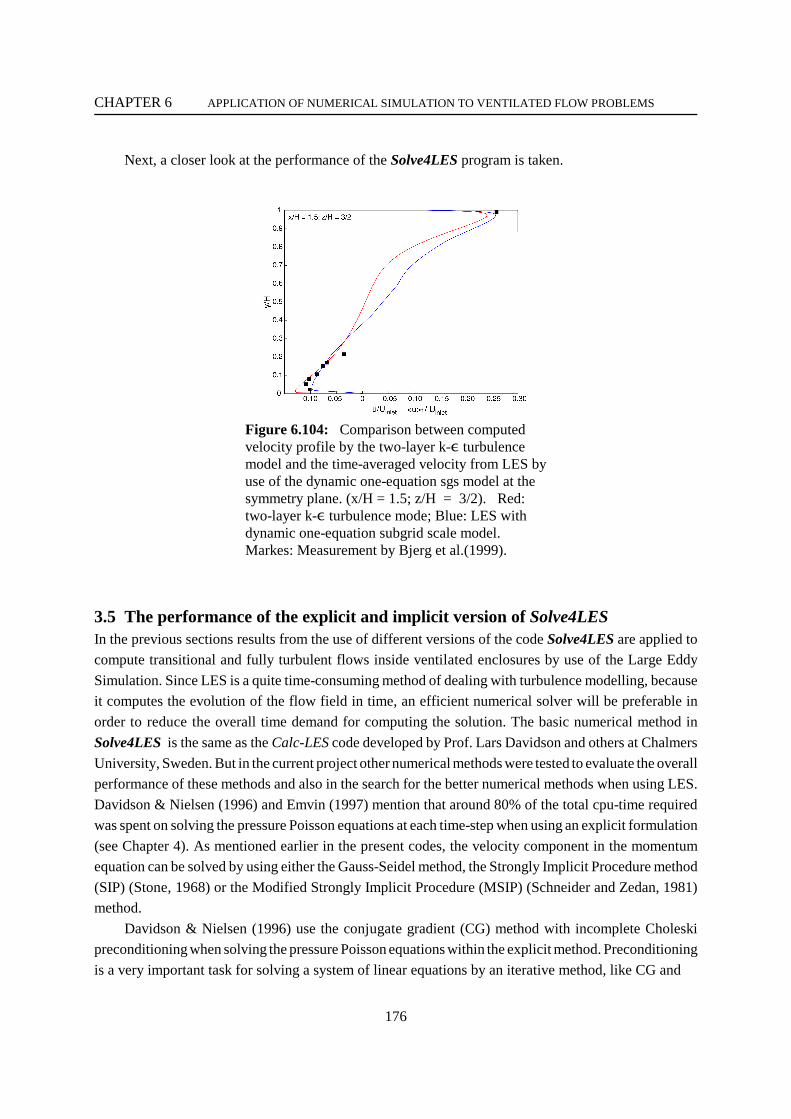
Finally in Figures 6.102 - 6.104 show the velocity profile comparing the two-layer k-I turbulencewithin Solve4kIIII and the time averaged velocity profile from the Large Eddy Simulation with the dynamicone-equation subgrid scale model to the measured data (Bjerg et al. (1999)).

Just below the ceiling at y/H = 0.99 and x/H = 1.5, both types of simulation agree well with themeasurement. Although for z/H = 3/2, the LES with the dynamic one-equation subgrid scale modelpredicts the jet peak velocity a little closer to the measurement. In the return flow the maximum velocityis also predicted quite well, compared to the experiments. The differences between the two-layer k-Iturbulence model and the LES is observed in the middle of the room, where the low velocity region exists.Unfortunately, no experimental data exist for that area of the room.

A very interesting point remains from these simulations when LES is used: Can LES predict theswitch-over of the inlet jet ? Since the present LES was only run for 1000 sec. and the measurements weremore than 10 times longer, this was not attempted in this project.


176

Figure 6.104: Comparison between computedvelocity profile by the two-layer k-I turbulencemodel and the time-averaged velocity from LES byuse of the dynamic one-equation sgs model at thesymmetry plane. (x/H = 1.5; z/H = 3/2). Red:two-layer k-I turbulence mode; Blue: LES withdynamic one-equation subgrid scale model.Markes: Measurement by Bjerg et al.(1999).

Next, a closer look at the performance of the Solve4LES program is taken.

3.5 The performance of the explicit and implicit version of Solve4LESIn the previous sections results from the use of different versions of the code Solve4LES are applied tocompute transitional and fully turbulent flows inside ventilated enclosures by use of the Large EddySimulation. Since LES is a quite time-consuming method of dealing with turbulence modelling, becauseit computes the evolution of the flow field in time, an efficient numerical solver will be preferable inorder to reduce the overall time demand for computing the solution. The basic numerical method inSolve4LES is the same as the Calc-LES code developed by Prof. Lars Davidson and others at ChalmersUniversity, Sweden. But in the current project other numerical methods were tested to evaluate the overallperformance of these methods and also in the search for the better numerical methods when using LES.Davidson & Nielsen (1996) and Emvin (1997) mention that around 80% of the total cpu-time requiredwas spent on solving the pressure Poisson equations at each time-step when using an explicit formulation(see Chapter 4). As mentioned earlier in the present codes, the velocity component in the momentumequation can be solved by using either the Gauss-Seidel method, the Strongly Implicit Procedure method(SIP) (Stone, 1968) or the Modified Strongly Implicit Procedure (MSIP) (Schneider and Zedan, 1981)method.

Davidson & Nielsen (1996) use the conjugate gradient (CG) method with incomplete Choleskipreconditioning when solving the pressure Poisson equations within the explicit method. Preconditioningis a very important task for solving a system of linear equations by an iterative method, like CG and


2SLAP: available from http://www.netlib.org/slap

3) SPARSKIT II available from http://www.cs.umn.edu/~saad

177

other Krylov subspace methods in other to accelerate the convergence rate. During the implementationof the explicit version of Solve4LES the same Sparse Linear Algebra Package (SLAP)2) as Davidson andNielsen (1996) were tested briefly, simulating the Annex 20 test case. The CFL number was kept below0.4, and only the Smagorinsky model was applied. The cpu-time per time step/grid point was found to2.6 × 10 - 4 (sec./grid point). The number of grid points used for this test were only 64×32×32 in the x-,y- and z-directions, respectively, and the cpu-time increased dramatically when larger number of gridpoints were used. This means that 95% of the total cpu-time per time step will be required to solve thepressure Poisson equations, although this explicit method has the advantage that the matrix arising fromthe discretion of the pressure Poisson equations will have the same coefficients, which implies that thecalculation of the preconditioning matrix only has to be carried out once within the first time step, byusing the SLAP package for the calculation of the incomplete Choleski preconditioner requiredapproximably the same time as 12 time steps during the Large Eddy Simulation. However, since thiscalculation will only be needed once, it represents only a fraction of the total computational time whenusing Large Eddy Simulation. In order to test the performance of other preconditioners, a separateimplementation of the Conjugate Gradient method together with an incomplete Choleski (IC)preconditioner, the ILUT (Saad, 1996) which combines incomplete factorization and a threshold strategyfor dropping the numerical fill-in values in the preconditioning matrix was implemented and tested. Thedropping residual was set at 10 -6 and number of fill-in’s were set at 7 (see Saad (1996) for furtherinformation). Moreover, the multilevel-like incomplete factorization method by Botta &Wubs (1999)named , the Matrix-Renumbering Incomplete LU factorization method (MRILU), which is able to achievenear grid independent convergence rate as also the multigrid method is know for was implemented andtested. Finally, a multigrid method (Llorente and Melson, 1998) was implemented and tested for both theexplicit and implicit versions of Solve4LES.

Some other important factors to be considered when different numerical methods are implementedare the computer architectural issues. The testing of different storage formats for the sparse banded matrixarising from the pressure Poisson equations like those mentioned in the SPARSKIT3) package can giveperformances between 4 and 52 Mflops on the currently used PC workstation. A technique to be used forimproving performance on most workstations may be the re-use of the cache-memory, which will oftenrequire some sort of re-ordering of the storage-structure or the sparse-matrix bandwidth minimization.This, however, has not been utilized in the current code. Improvements to the code were made by carefullloop unrolling (the creation of fat loop), reduction of procedure, function calls within loops (by in-liningfunctions and even procedure calls), and the reduction of branches (conditional statements like if-then)within loops. The original matrix is stores as a banded sparse matrix and the preconditioning matrix usingcompressed row format (Saad, 1996). The same code running on vector supercomputers and cache-basedRISC workstations will usually involve severe problems regarding the overall performance. This was also


4Linpack benchmark: is used to solve a dense system of linear equations. It reflects theperfor-mance of a computer for solving a dense system of linear equations, and since the problem isvery regular, the performance achieved will be quite high, and the performance numbers will give agood representation of the peak performance The sizes of the dense system of linear equations will usually be 100 × 100 and 1000 × 1000. See http://www.netlib.org/benchmark/index.html foradditional information about the Linpack benchmark program and software.

178

illustrated with the LESROOM code since this was optimized for the Cray vector supercomputer bymeans of a data structure that favours long vector lengths that could easily be pipelined by this kind ofprocessor. Comparing the performance of LESROOM between the Cray and the PC based on the Mflopsvalues, the ratio was between 14 - 18 in favour of the Cray. Even if the Linpack 4) benchmark shows aratio between the Cray and the currently used PC workstation to be 3.6 and 3, respectively, when thesizes of the dense system of linear equations are 100×100 and 1000×1000.

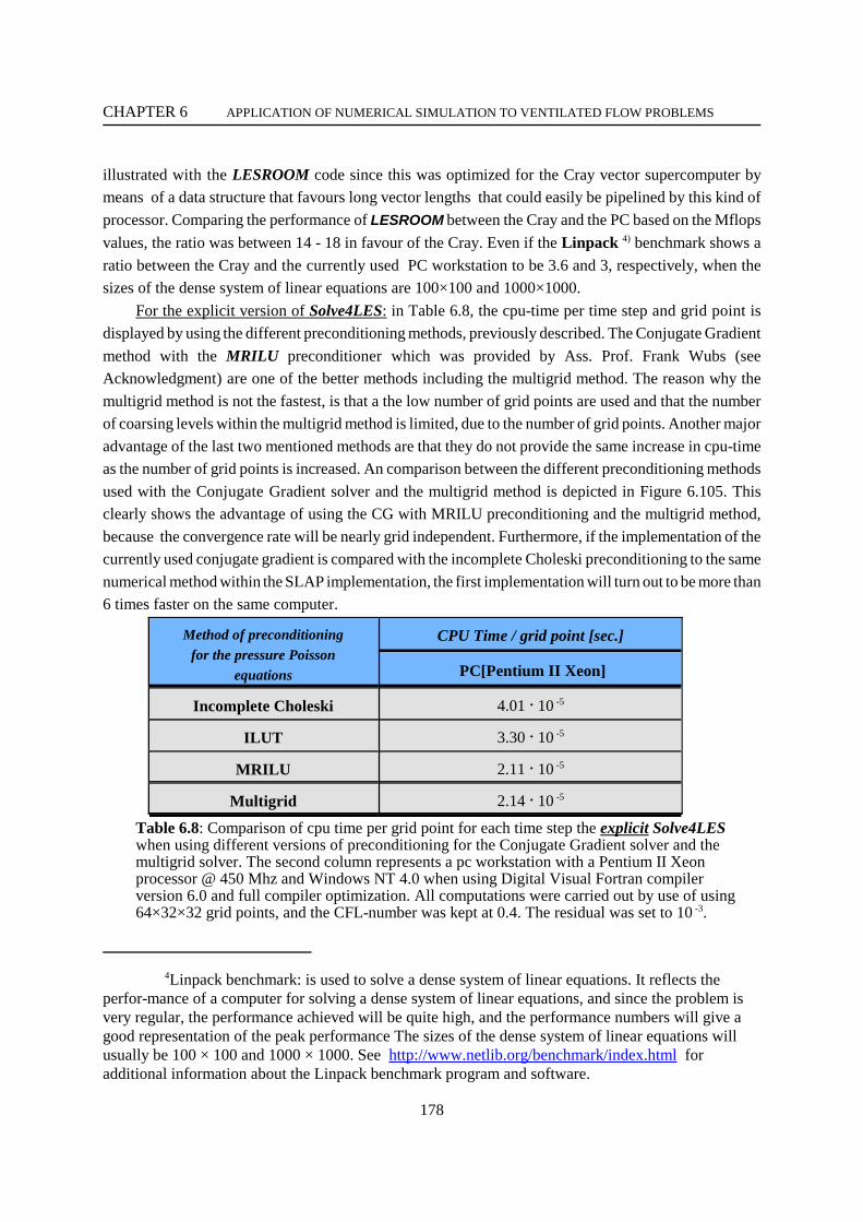
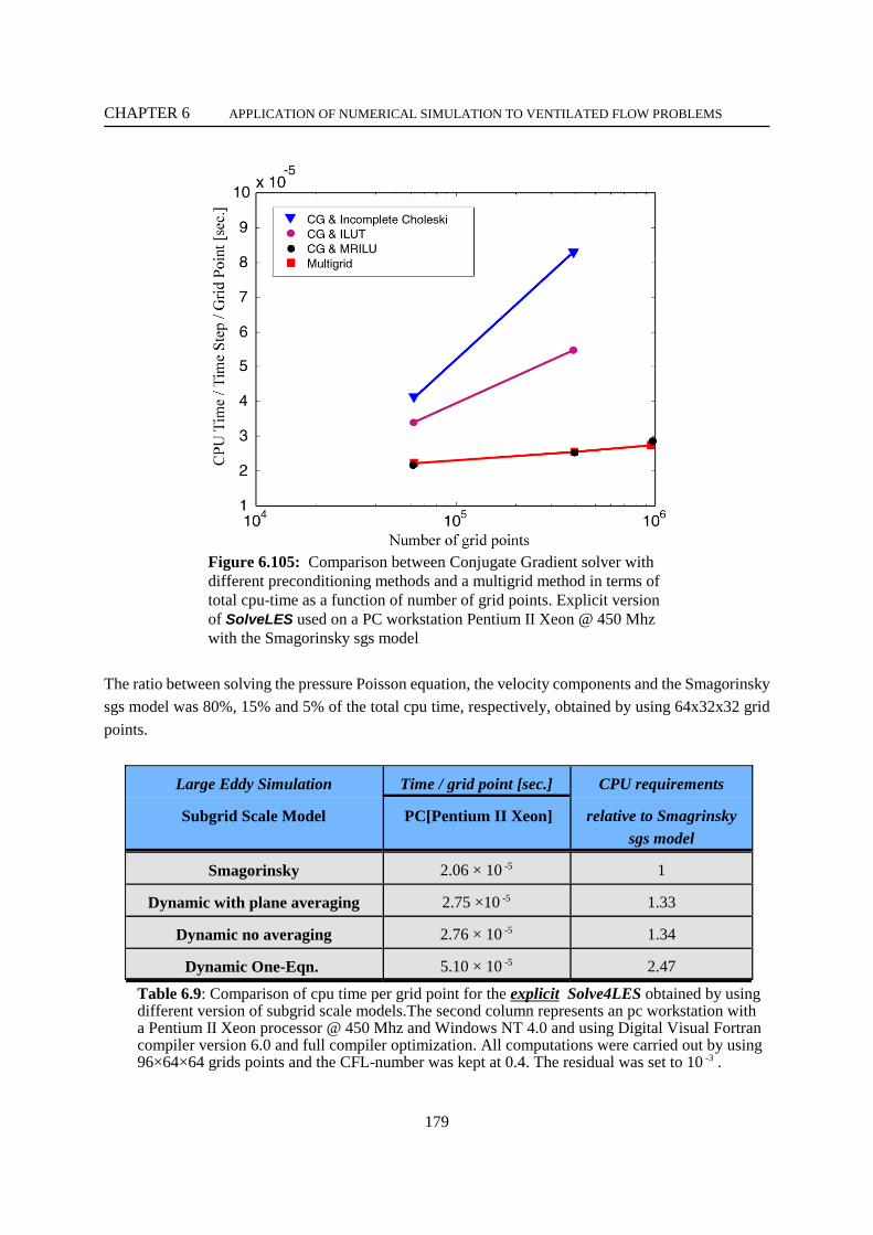
For the explicit version of Solve4LES: in Table 6.8, the cpu-time per time step and grid point isdisplayed by using the different preconditioning methods, previously described. The Conjugate Gradientmethod with the MRILU preconditioner which was provided by Ass. Prof. Frank Wubs (seeAcknowledgment) are one of the better methods including the multigrid method. The reason why themultigrid method is not the fastest, is that a the low number of grid points are used and that the numberof coarsing levels within the multigrid method is limited, due to the number of grid points. Another majoradvantage of the last two mentioned methods are that they do not provide the same increase in cpu-timeas the number of grid points is increased. An comparison between the different preconditioning methodsused with the Conjugate Gradient solver and the multigrid method is depicted in Figure 6.105. Thisclearly shows the advantage of using the CG with MRILU preconditioning and the multigrid method,because the convergence rate will be nearly grid independent. Furthermore, if the implementation of thecurrently used conjugate gradient is compared with the incomplete Choleski preconditioning to the samenumerical method within the SLAP implementation, the first implementation will turn out to be more than6 times faster on the same computer.

Method of preconditioningfor the pressure Poisson

equations

CPU Time / grid point [sec.]

PC[Pentium II Xeon]

Incomplete Choleski 4.01 l 10 -5

ILUT 3.30 l 10 -5

MRILU 2.11 l 10 -5

Multigrid 2.14 l 10 -5

Table 6.8: Comparison of cpu time per grid point for each time step the explicit Solve4LES when using different versions of preconditioning for the Conjugate Gradient solver and the multigrid solver. The second column represents a pc workstation with a Pentium II Xeonprocessor @ 450 Mhz and Windows NT 4.0 when using Digital Visual Fortran compilerversion 6.0 and full compiler optimization. All computations were carried out by use of using64×32×32 grid points, and the CFL-number was kept at 0.4. The residual was set to 10 -3.


179

Figure 6.105: Comparison between Conjugate Gradient solver withdifferent preconditioning methods and a multigrid method in terms oftotal cpu-time as a function of number of grid points. Explicit versionof SolveLES used on a PC workstation Pentium II Xeon @ 450 Mhzwith the Smagorinsky sgs model

The ratio between solving the pressure Poisson equation, the velocity components and the Smagorinskysgs model was 80%, 15% and 5% of the total cpu time, respectively, obtained by using 64x32x32 gridpoints.

Large Eddy Simulation Time / grid point [sec.] CPU requirements

Subgrid Scale Model PC[Pentium II Xeon] relative to Smagrinskysgs model

Smagorinsky 2.06 × 10 -5 1

Dynamic with plane averaging 2.75 ×10 -5 1.33

Dynamic no averaging 2.76 × 10 -5 1.34

Dynamic One-Eqn. 5.10 × 10 -5 2.47

Table 6.9: Comparison of cpu time per grid point for the explicit Solve4LES obtained by usingdifferent version of subgrid scale models.The second column represents an pc workstation witha Pentium II Xeon processor @ 450 Mhz and Windows NT 4.0 and using Digital Visual Fortrancompiler version 6.0 and full compiler optimization. All computations were carried out by using96×64×64 grids points and the CFL-number was kept at 0.4. The residual was set to 10 -3 .


180

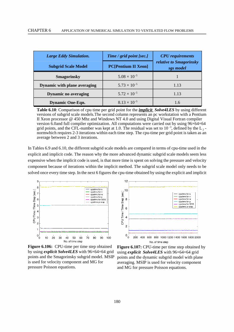
Figure 6.106: CPU-time per time step obtainedby using explicit Solve4LES with 96×64×64 gridpoints and the Smagorinsky subgrid model. MSIPis used for velocity component and MG forpressure Poisson equations.

Figure 6.107: CPU-time per time step obtained byusing explicit Solve4LES with 96×64×64 gridpoints and the dynamic subgrid model with planeaveraging. MSIP is used for velocity componentand MG for pressure Poisson equations.

Large Eddy Simulation. Time / grid point [sec.] CPU requirementsrelative to Smagorinsky

sgs modelSubgrid Scale Model PC[Pentium II Xeon]

Smagorinsky 5.08 × 10 -5 1

Dynamic with plane averaging 5.73 × 10 -5 1.13

Dynamic no averaging 5.72 × 10 -5 1.13

Dynamic One-Eqn. 8.13 × 10 -5 1.6

Table 6.10: Comparison of cpu time per grid point for the implicit Solve4LES by using differentversions of subgrid scale models.The second column represents an pc workstation with a PentiumII Xeon processor @ 450 Mhz and Windows NT 4.0 and using Digital Visual Fortran compilerversion 6.0and full compiler optimization. All computations were carried out by using 96×64×64grid points, and the CFL-number was kept at 1.0. The residual was set to 10 -3, defined by the L 2 -normwhich requires 2-3 iterations within each time step. The cpu-time per grid point is taken as anaverage between 2 and 3 iterations.

In Tables 6.9 and 6.10, the different subgrid scale models are compared in terms of cpu-time used in theexplicit and implicit code. The reason why the more advanced dynamic subgrid scale models seem lessexpensive when the implicit code is used, is that more time is spent on solving the pressure and velocitycomponent because of iterations within the implicit method. The subgrid scale model only needs to besolved once every time step. In the next 6 figures the cpu-time obtained by using the explicit and implicit


181

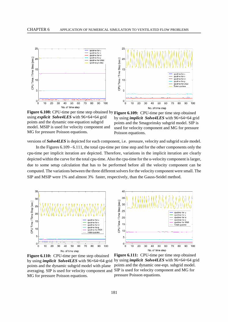
Figure 6.108: CPU-time per time step obtained byusing explicit Solve4LES with 96×64×64 gridpoints and the dynamic one-equation subgridmodel. MSIP is used for velocity component andMG for pressure Poisson equations.

Figure 6.109: CPU-time per time step obtainedby using implicit Solve4LES with 96×64×64 gridpoints and the Smagorinsky subgrid model. SIP isused for velocity component and MG for pressurePoisson equations.

Figure 6.110: CPU-time per time step obtainedby using implicit Solve4LES with 96×64×64 gridpoints and the dynamic subgrid model with planeaveraging. SIP is used for velocity component andMG for pressure Poisson equations.

Figure 6.111: CPU-time per time step obtainedby using implicit Solve4LES with 96×64×64 gridpoints and the dynamic one-eqn. subgrid model.SIP is used for velocity component and MG forpressure Poisson equations.

versions of Solve4LES is depicted for each component, i.e. pressure, velocity and subgrid scale model.In the Figures 6.109 - 6.111, the total cpu-time per time step and for the other components only the

cpu-time per implicit iteration are depicted. Therefore, variations in the implicit iteration are clearlydepicted within the curve for the total cpu-time. Also the cpu-time for the u-velocity component is larger,due to some setup calculation that has to be performed before all the velocity component can becomputed. The variations between the three different solvers for the velocity component were small. TheSIP and MSIP were 1% and almost 3% faster, respectively, than the Gauss-Seidel method.


5SPECMARK: see http://www.specbench.org for further information.

182

From the depicted results on the requirement of cpu-time when using the currently describedimplementation featuring either an explicit or an implicit method of time advancement, Large EddySimulation is still quite time-consuming compared to other methods of turbulence modelling where theflow field is decomposed into a steady and a fluctuating part, the Reynolds Averaging, although theimplicit method has the potential to even larger time steps than the currently used limits of one. But itcould be questionable to use large time steps in a transitional evolving flow field. This has so far not beentested. But LES is capable of providing much more information about the flow field, although notsuperior when mean averaging velocity profiles are compared. Furthermore, LES is capable of computinga solution to a flow field that is not fully developed, thus making it very attractive for many ventilationproblems where the Reynolds number is often below 5000 and for many cases within the transitional flowrange.

Finally, the reported cpu measurement on the PC workstation with a Pentium II, Xeon processor,which is approximable one year behind the latest processor trend, could be reduced by upgrading to thelatest processor. This modern processor will be nearly capable of reducing the cpu-time by a factor of twoand a factor of almost four when the latest UNIX-based workstation with the Alpha processor is used.This assumption is based on the currently available specmark5) ( Spec_fp95 ) numbers for floating pointspeeds. The additional use of parallel computer would certainly make Large Eddy Simulations attractive.But the interaction between implementation, the numerical methods, the architectural issues, and thecompiler technology remains a challenge. The easy gains in computational speed are over.

Documents

CHAPTER 6 APPLICATION OF NUMERICAL …homes.civil.aau.dk/.../Bennetsen_JC/chap6_del_5.pdfCHAPTER 6 APPLICATION OF NUMERICAL SIMULATION TO VENTILATED FLOW PROBLEMS 1) Personal communication