Embed Size (px)
Citation preview

Chapter 6
Alternatives to Expected Utility
Theory
In this lecture, I describe some well-known experimental evidence against the expected
utility theory and the alternative theories developed in order to accommodate these
experiments. (I have posted a comprehensive survey on the class web page.)
6.1 Calibration Paradox
Under expected utility maximization, a decision maker is approximately risk neutral
against a small risk whenever his utility function is differentiable at his initial wealth
level, a condition that is satisfied for almost all initial wealth levels when the decision
maker is risk averse. For example, she is always willing to invest some positive amount in
an asset with positive expected utility. An implication of this result is that, if a decision
maker is rejecting some small amount of risk with positive gain for a range of wealth
levels, then he will not take any large risk even when there are very large potential gains,
refusing to make any reasonable investment.
To illustrate this, suppose first that DM has constant absolute risk-aversion and
plausibly rejects a gamble ($1 $ − 1; 06; 04) that gives 1 dollar with probability = 06
and −1 dollar with probability 1 − . Then, his absolute risk aversion must be at least
ln (32), i.e.,
≥ ln ( (1 − )) = ln 32
49

50 CHAPTER 6. ALTERNATIVES TO EXPECTED UTILITY THEORY
But such a decision maker would reject any gamble that involves a loss of 2 dollars with
probability 1/2, no matter how larger the gains are with the remaining probabilty 1/2.
Indeed, the payoff from such a gamble could be at most
1 1 1 − exp (− · (−2)) = 1 − (32)
2 = −18
2 2
which is clearly less than 0, the expected utility from 0. (The utility function is () =
1 − exp (−).) That is, if we calibrate a decision maker’s utility function using constant risk-aversion
from a plausible observation of rejecting a gamble ($1 $ − 1; 06; 04), we then reach to
the utterly implausible conclusion that the decision maker will not take any gamble
that involes just 2 dollars loss with probability 1/2. It is tempting to take this as a
critique of CARA utilities. Afterall, one expects absolute risk aversion to be decreasing
(as in constant relative risk aversion), and CARA utilities used only for tractability of
theoretical exercises. This is not the case.
Rabin illustrates for any expected utility maximizer that if she would reject such
gambles for a reasonably small interval [ − 100 + 100] of initial wealth levels, he will
be rejecting any reasonable large gambles that one faces in real life, e.g. when she buys
a house or starts up a new business. The idea is quite simple (once one is told). If
she rejects ($1 $ − 1; 06; 04) for all initial weath levels in [ − 100 + 100], then her
absolute risk aversion throughout that interval is at least ln (32). That gives enough
curviture over that interval to prohibit any risk taking behavior with large stakes. The
illustration if this is left as an exercise.
Exercise 6.1 Ann is a risk-averse expected utility maximizer with an increasing util-
ity function : R → R. She is indifferent between accepting and rejecting a lottery
($1−$1; 06 04) that gives $1 (gain) with probability = 06 and −$1 (loss) with prob-ability (1 − ) for all initial wealth levels in [0 − 100 0 + 100]. Find the smallest
for which Ann is willing to accept a lottery that gives $ (gain) with probability 1/2 and
−$ = −$100 000 (loss) with probability 1/2 consistent with above information. That
is, find
∗ = min {| (+ 0) + (−+ 0) ≥ (0) ∈ }
where is the set of utility functions described above.

51 6.2. ALLAIS PARADOX AND WEIGHTED UTILITY
6.2 Allais Paradox and Weighted Utility
Imagine yourself choosing between the following two alternatives:
A Win 1 million dollar for sure.
B Win 5 million dollar with 10% chance, 1 million dollar with 89%, nothing with 1%.
Which one would you choose? In many surveys, subjects who were offered these
alternatives chose A. It seems that they did not want to risk the opportunity of having
a million dollar for a 10% chance of having five million dollar instead. Now consider the
following two alternatives:
C Win $1M with 11% chance, nothing with 89%.
D Win $5M with 10% chance, nothing with 90%.
It seems that the probability of winning the prize is similar for the two alternatives,
while the prizes are substantially different. Hence, it seems reasonable to choose the
higher prize, choosing D rather than C. Indeed, in surveys, the subjects choose D.
Unfortunately, for an expected utility maximizer, the trade of between A and B is
identical to the trade of between C and D, and he prefers A to B if and only if he prefers
C to D. To see this, note that for an expected utility maximizer with utility function ,
A is better than B if and only if (1) 01 (5) + 089 (1), i.e.,
011 (1) 01 (5) (6.1)
where the unit of money is million dollar, and the utility from 0 is normalized to 0. But
for such an expected utility maximizer, C is better than D if and only if (6.1) holds.
The above experiment against the expected utility theory has been designed by Allais.
It illustrates for the subjects surveyed that the indifference curves are not parallel, and
hence the independence axiom is violated. This is illustrated in Figure 6.1. As shown
in the figure, the lines connecting A to B and C to D are parallel to each other. Since
A is better than B, the indifference curve through A is steeper than the line connecting
A to B. Since D is better than C, the indifference curve through C is flatter than the
line connecting C to D. Therefore, the indifference curve through A is steeper than the
indifference curve through C.

52 CHAPTER 6. ALTERNATIVES TO EXPECTED UTILITY THEORY
Pr($0)
Pr($5)
1
1
0
A∙ ∙∙B
C
D
∙
B’∙
Indifference curves
Figure 6.1: Allais Paradox. The prizes are in terms of million dollars. Probability of 0
is on the horizontal axis; the probability of 5 is on the vertical axis, and the remaining
probability goes to the intermediate prize 1.
A series of other experiments also suggested that the indifference curves are not
parallel and "fan out’ as in the figure. Consequently, decision theorists have developed
many alternative theories in which the indifference curves are not parallel. These theories
often assume that the indifference curves are straight lines, called betweenness.
A prominent theory among these assumes that the indifference curves are straight
lines that fan out from a single origin. This theory is called Weighted Utility Theory, as
it assumes the following general form for the utility from a lottery :
P () = (| ) ()
∈
where () ()
(| ) = P ∈ () ()
for some function : → R. Here, the utilities are weighted according to not only the
probabilities of the consequences but also according to the consequences themselves. Of
course, if is constant, the weighting is done only according to the probabilities, as in
the expected utility theory.
Exercise 6.2 Check that under the weighted utility theory, the indifference curves are
straight lines, but the slope of the indifference curves differ when is not constant. Tak-

53 6.2. ALLAIS PARADOX AND WEIGHTED UTILITY
1.0 w 0.8
0.6
0.4
0.2
0.0
p 0.0 0.1 0.2 0.3 0.4 0.5 0.6 0.7 0.8 0.9 1.0
Figure 6.2: Probability Weighting Function; () = −(− ln ) for some ∈ (0 1).
ing with three elements, characterize the functions and under which the indifference
sets fan out as in the Allais paradox.
In the weighted utility theory, the decision maker distorts the probabilities using the
consequences themselves and the whole probability vector . In general, probabilities
need to be distorted if one wants to incorporate Allais paradox in expected utility theory.
A prominent theory that distorts the probabilities to this end is rank-dependent expected
utility theory. In this theory, one first ranks the consequences in the order of increasing
utility. He then applies probability weighting function to the cumulative distribution
function and distorts it to a new cumulative distribution function ◦ . One then
finally uses expected utility under the distorted probabilities in order to evaluate the
lottery. The resulting value function is Z (|) = () ( ()) (6.2)
The survey results in the Allais paradox suggest that the subjects overestimate the
small probability events with extreme value, such as getting nothing with a small proba-
bility. In order to capture such a behavior, one often uses an inverted shaped probabil-
ity weighting function as in Figure 6.2. Here, is an increasing function with (0) = 0
and (1) = 1, and it crosses the diagonal once at some ∗ . The general functional form
() = −(− ln ) for some ∈ (0 1) has many desirable properties.
Example 6.1 Consider the lotteries in the Allais paradox. Set (0) = 0 and (1) = 1.

54 CHAPTER 6. ALTERNATIVES TO EXPECTED UTILITY THEORY
The value of lottery B is computed as follows:
(|) = (001) (0) + [ (09) − (001)] (1) + (1 − (09)) (5)
= (09) − (001) + (1 − (09)) (5)
Similarly, the values of the other lotteries are
(|) = 1
(|) = 1 − (089)
(|) = (1 − (09)) (5)
Now take (5) ∈ (1 (− 1)) and () = −(− ln ) . Note that
lim (|) = 1 (1 − 1) (5) = lim (|) = lim (|) 1−1 = lim (|) →0 →0 →0 →0
Thus, for small , the preferences are as in the Allais paradox.
6.3 Ellsberg Paradox and Ambiguity Aversion
Consider an urn that contains 99 balls, colored Red, Black and Green. We know that
there are exactly 33 Red balls, but the exact number of the other colors is not known.
A ball is randomly drawn from this urn. You choose a color.
• If the ball is of the color you choose, you win $1. What color would you choose?
• If the ball is not of the color you choose, you win $1. What color would you
choose?
When different subjects are asked these questions, an overwhelming majority of them
chose red ball in both questions. That is to say, in the first question, an overwhelming
majority of the subjects bet on the event that the ball is red, and in the second question
an overwhelming majority bet that the ball is not red. This can be taken as an evidence
against the expected utility theory because an expected utility maximizer cannot have
a strict preference in both questions. Indeed, if the probability of colors red, black, and
green are , , and , respectively, then having a strict preference for red in the first
question means that
and .

55 6.3. ELLSBERG PARADOX AND AMBIGUITY AVERSION
A strict preference for red in the second question means that
1− 1− and 1− 1− ,
i.e.,
and ,
a clear contradiction.
This is called Ellsberg Paradox. Note that this is an evidence against the expected
utility theory as formulated by Savage, assuming that the money is the consequence.
In particular, it contradicts the basic assumption that the individuals have well-defined
beliefs that give a well-defined probability for each consequence under each act. Within
the framework of von Neumann and Morgenstern, this could be taken as an evidence
against the fundamental modeling assumption that compound lotteries are reduced to
the simple lotteries.
Suppose that the decision maker believes that the each ball is equally likely to be
drawn. Given the number of black balls, the probability of each color is as follows:
Pr (|) = 13
Pr (|) = 99
Pr (|) = 23− 99
(Here, means that the ball is red; means that the ball is black, and means that
the ball is green.) Savage assumes that the decision maker has a belief about . For
every given belief about , each bet yields a compound lottery. For example, the
compound lotteries given by betting on the event that the ball is red and betting on
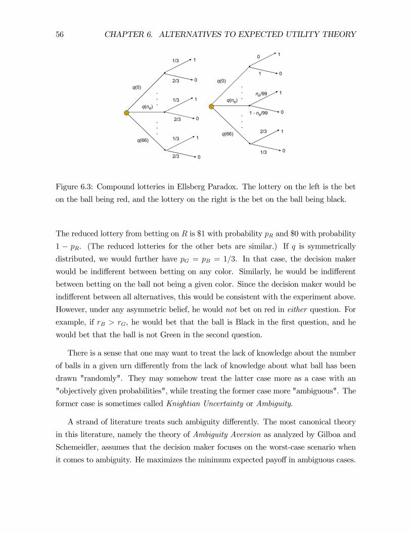
the event that the ball is black are plotted in Figure 6.3.
In expected utility theory, one further assumes that the compound lotteries are re-
duced to simple lotteries. This reduction yields the following probabilities for the color
of the ball:
= 13
66X = () 99
=0
= 23−
56 CHAPTER 6. ALTERNATIVES TO EXPECTED UTILITY THEORY
.
.
.
.
.
.
q(0)
q(nB)
q(66)
1
0
1
0
1
0
.
.
.
.
.
.
q(0)
q(nB)
q(66)
1
0
1
1/3
1/3
1/3
2/3
2/3
2/3
0
1
1 - nB/99
nB/99
2/3
1/3
0
1
0
Figure 6.3: Compound lotteries in Ellsberg Paradox. The lottery on the left is the bet
on the ball being red, and the lottery on the right is the bet on the ball being black.
The reduced lottery from betting on is $1 with probability and $0 with probability
1 − . (The reduced lotteries for the other bets are similar.) If is symmetrically
distributed, we would further have = = 13. In that case, the decision maker
would be indifferent between betting on any color. Similarly, he would be indifferent
between betting on the ball not being a given color. Since the decision maker would be
indifferent between all alternatives, this would be consistent with the experiment above.
However, under any asymmetric belief, he would not bet on red in either question. For
example, if , he would bet that the ball is Black in the first question, and he
would bet that the ball is not Green in the second question.
There is a sense that one may want to treat the lack of knowledge about the number
of balls in a given urn differently from the lack of knowledge about what ball has been
drawn "randomly". They may somehow treat the latter case more as a case with an
"objectively given probabilities", while treating the former case more "ambiguous". The
former case is sometimes called Knightian Uncertainty or Ambiguity.
A strand of literature treats such ambiguity differently. The most canonical theory
in this literature, namely the theory of Ambiguity Aversion as analyzed by Gilboa and
Schemeidler, assumes that the decision maker focuses on the worst-case scenario when
it comes to ambiguity. He maximizes the minimum expected payoff in ambiguous cases.
57 6.3. ELLSBERG PARADOX AND AMBIGUITY AVERSION
For example, he takes the values of betting on events and as
() = min 13 = 13
() = min99 = 0
() = min [23− 99] = 0
Hence, in the first question, an ambiguity averse decision maker chooses to bet on the
event that the ball is red. On the other hand, the value of betting on the event that the
ball is not a given color is given by
() = min 23 = 23
() = min [1− 99] = 13
() = min {1− [23− 99]} = 13
where and denote the complements of , , and , respectively. Hence,
in the second question, an ambiguity-averse decision maker chooses to bet that the ball
is not red.
More generally, theory of ambiguity aversion assumes that there are multiple priors
∈ on state space , the set is the range of ambiguity. Given any , an act yields R an expected utility [ () |] = ( ()) (), where the outcome of an act can be a
lottery as in the Anscombe and Aumann model. For any given act , the worst possible
expected payoff is
() = min [ () |] ∈
The decision maker maximizes this minimum expected utility. His choice function is Z () = argmaxmin ( ()) ()
∈ ∈
Note that this is a theory of an irrational decision maker, who mistakenly assumes that
his choices affect the underlying state of the world, which is given.
Focusing on the worst-case scenarios is clearly an extreme behavior and yields a
useless guide for behavior in many real-world problems. For, under a full support as-
sumption, the worst case scenario is the worst consequence, making the decision maker
indifferent between all such acts. An alternative to above theory introduces the beliefs
about the ambiguous states but treats these probabilities differently. It introduces a

58 CHAPTER 6. ALTERNATIVES TO EXPECTED UTILITY THEORY
probability distribution on and assumes that the decision maker maximizes Z µZ ¶ () = [ ( ())] = ( ()) () ()
where : R → R is a concave function. Hence, the choice function is Z µZ ¶ () = arg max [ ( ())] = arg max ( ()) () ()
∈ ∈
This theory is called Smooth Ambiguity Aversion. The ambiguity aversion is a particular
−limit in which gets extremely concave. For example, if we take () = − and
let → ∞, we would get the ambiguity aversion in the sense of max min. When is
degenerate (or equivalently is singleton), this reduces to the standard expected utility
theory.
While Ellsberg paradox illustrates that the decision maker does not reduce the un-
certainty about the number of balls into a simple probability distrbution on winning,
it is not clear whether she does it because she is ambiguity averse or whether she has
difficilty in reducing compound lotteries to simple lotteries (failure of ROCL), due to
perhaps some form of bounded rationality. Clearly, the two alternative theories have
very different implication to the decision making in complex environments in economics.
Fortunately, there is a simple test. One can provide the probabilities to decision maker
(and describe the problem differently) so that the problem is a given compound lotteries.
If the reason were ambiguity aversion, then DM would now act as an expected utility
maximizer (as there is no ambguity). If the reason were failure of ROCL, then he would
remain to differ from expected utility maximization, still behaving as in Ellsberg para-
dox. Indeed, Yoram Halevy has run such an experiment. His results are in Table I. With
few exceptions, subjects deviated from expected utility theory (ambiguity neutrality) if
and only if they failed to reduce compound lotteries (ROCL). Indeed, there were only
one subject who could reduce the compound lotteries and would deviate from ambiguity
neutrality. That is the only subject who fits the ambguity aversion model.
6.4 Framing
The theories so far all assumed that the decision is not affected by the way the decision
problem is formulated. Actually, in many experiments, the way the problem is formu-
lated has a large impact on the decision. This phenomenon is called framing effect. The

59 6.4. FRAMING
Figure 6.4:
following example, due to Kahneman and Tversky, illustrates this fact. They have asked
to a group of subjects the following question.
An outbreak of a disease is about to kill 600 people. There are two
possible treatments A and B with the following results.
A 400 people die.
B Nobody dies with 1/3 chance, 600 people die with 2/3 chance.
Which treatment would you choose?
In response to this question, 78% of subjects have picked treatment B. To a different
group of subjects, they have offered the following treatments:
C 200 people saved.
D All saved with 1/3 chance, nobody saved with 2/3 chance.
This time, only 28% of subjects have picked D. But clearly, apart from wording, A is
equivalent to C, and B is equivalent to D. By changing the wording of letting 400 people
die to saving 200 people altered the way the subjects approached the problem.
Unlike the previous theories, the next theory allows framing.

60 CHAPTER 6. ALTERNATIVES TO EXPECTED UTILITY THEORY
6.5 Prospect Theory
Based on survey data, Kahneman and Tversky developed a theory of decision making
in which the decision maker distorts the probabilities of events, as in rank-dependent
expected utility, and evaluates the consequences according to a reference-dependent util-
ity function, which treats "gains" differently from the "losses". In addition, Kahneman
and Tversky allow the decision maker to "edit" the problem in a way to simplify the
problem before applying the above procedure. There are two versions of the theory. In
the sequel, I describe the Cumulative Prospect Theory.
In this theory, the reference point 0 plays a central role. The consequences that are
above 0 are considered gains and the ones below 0 are considered losses. In the first
stage, using a probability weighting function as in the rank-dependent expected utility,
one distorts the cumulative distributions of gains and losses separately. The probability
weighting is done started from the extremes. Hence, the resulting cumulative density
function for the losses is
(|0) = 1− (1− ()) for ≤ 0
The resulting cumulative density function for the gains is
(|0) = ( ()) for ≥ 0
In the second stage, he evaluates each consequence according to a reference-dependent
utility function
(|0) = ( − 0)
where is an increasing function with the following properties (see Figure 6.5 for an
illustration):
• is concave on the positive numbers, i.e., the decision maker is risk-averse towards
gains;
• is convex on the negative numbers, i.e., the decision maker is risk-seeking towards
losses;
• there is a kink at 0, so that the decision maker is affected by small losses more
than he is affected by equal amount of gains (loss aversion).

61 6.5. PROSPECT THEORY
v
x
Figure 6.5: Value Function in Prospect Theory
After distortion of probabilities and reference-dependent evaluation of consequences,
the decision maker applies expected utility. The resulting value function for any given
lottery is Z ( | 0 ) = (|0) (|0) Z Z
= ( − 0) (1 − (1 − ())) + ( − 0) ( ()) 0 0
Exercise 6.3 Take () = and ( √ if ≥ 0
() = √ −2 − if 0
Consider a lottery ticket that pays 106 with probability 10−6 . How much is the decision
maker willing to pay to buy the lottery ticket. Now suppose that there is a risk in the
decision maker’s wealth, so that he can lose 106 with probability 10−6. (For example, his
house can burn.) How much is he willing to pay for a full insurance against this risk?
If both insurance and lottery ticket are sold by a risk neutral seller, what is the range of
individually rational prices for each of them?
Notice that in prospect theory, the decision is greatly affected by the reference point.
If the reference is taken to be the smallest consequence available in the lotteries, the

62 CHAPTER 6. ALTERNATIVES TO EXPECTED UTILITY THEORY
individual is risk averse (and is a rank-dependent expected utility maximizer). If the
reference is taken to be the largest consequence available in the lotteries, he is now
risk-seeking (and a rank-dependent expected utility maximizer in the reverse order). If
one can affect the reference point by framing the problem, he can have a great impact
on the decision. In that case, the individuals in prospect theory are prone to framing.
Although the reference point is very important for the theories, it is not clear what it
should be (and it is left to be determined by the context).1
Exercise 6.4 Take zero wealth as the reference point in the previous exercise.
Exercise 6.5 Take () = and ( if ≥ 0
() = otherwise
for some ≥ 1. Take the initial wealth level as the reference point. For every initial
wealth level, DM is indifferent between accepting and rejecting a lottery that gives $1
(gain) with probability = 06 and −$1 (loss) with probability (1 − ). Find the smallest
for which DM is willing to accept a lottery that gives $ (gain) with probability 1/2
and −$ = −$100 000 (loss) with probability 1/2 consistent with above information.
1There are some recent studies that suggest possible alternatives as the reference point.

MIT OpenCourseWarehttp://ocw.mit.edu
14.123 Microeconomic Theory IIISpring 2015
For information about citing these materials or our Terms of Use, visit: http://ocw.mit.edu/terms.


![The Predictive Utility of Generalized Expected Utility ...1].pdfEconometrica, Vol. 62, No. 6 (November, 1994), 1251-1289 THE PREDICTIVE UTILITY OF GENERALIZED EXPECTED UTILITY THEORIES](https://img.pdfslide.us/doc/110x75/5f3062794b20c364a743450f/the-predictive-utility-of-generalized-expected-utility-1pdf-econometrica.jpg)