Embed Size (px)
Citation preview

Copyrighted (Textbook) Fei Hu and Xiaojun Cao, Wireless Sensor Networks: Principles and Practice, CRC Press Page 1
Chapter 5: Transport Layer in Wireless Sensor Networks
As we recall from general network layers concept, the major tasks of Transport Layer is:
(1) to guarantee the reliable transmission of network packets through end-to-end retransmissions
or other strategies, and (2) to reduce or avoid the network congestion due to too much traffic
flowing in the routers or other relay points. TCP is used in Internet. However, we cannot use
TCP in WSN transport layer design. This chapter will explain WSN transport layer design
requirements and some good protocol examples.
5.1 Introduction
We can summarize the requirements of a transport layer protocol for sensor networks as
When you design a Transport Layer protocol for any network, it typically has 2 tasks: (1) It is responsible for end-to-end reliable transmission (i.e. no packet loss) instead of hop-to-hop reliable transmission (which is a MAC layer task). However, you could use hop-to-hop strategies to achieve end-to-end reliability. For instance, later on, we will discuss some WSN transport schemes that use hop-to-hop packet loss recovery to achieve end-to-end reliability. (2) A Transport Layer protocol should also take care of network congestion issues such as how to detect the congestion places and how to avoid those congestion events. Although the above 2 tasks are supposed to be implemented in the same transport protocol, some transport schemes only focus on one of them (either reliability or congestion issues). This is acceptable. However, we point out that it is not a complete transport protocol if only one of them is achieved.

Copyrighted (Textbook) Fei Hu and Xiaojun Cao, Wireless Sensor Networks: Principles and Practice, CRC Press Page 2
follows: [YIyer05]
1) Generic design: The WSN transport layer protocol should be independent of the
application, Network and MAC layer protocols. If a transport layer heavily depends on network
topology assumptions (such as a tree-based architecture), it may not be suitable to some
applications that use a flat topology.
2) Heterogeneous data flow support: A transport protocol should support both continuous
and event-driven flows in the same network. Continuous (i.e. streaming) data needs to use fast
response rate control algorithms to limit the stream flow speed in order to reduce congestion.
Event-driven flows have lower requirements on the rate control sensibility. But it requires a
highly reliable event capture (i.e. no data loss).
3) Controlled variable reliability: Some applications require complete reliability while
others might tolerate the loss of a few packets. The transport layer protocol should leverage this
fact and conserve energy at the nodes. For instance, if the system doesn’t need 100% packet
arrival rate, we may not invoke packet retransmission scheme.
4) Congestion detection and avoidance: The congestion detection and avoidance
mechanism is the most important design in a transport protocol. Congestion detection is not so
easy in WSNs because the congestion only exists in some specific “hot spots” where traffic
amount is significantly higher than other places. But how do we quickly detect those “hot spots”?
5) Base station controlled network: Since sensor nodes are energy constrained and
limited in computational capabilities, majority of the functionalities and computation intensive
tasks should be performed by the base station. However, if we could distribute some tasks in
sensors, we could obtain a better congestion avoidance effect since it is the sensors that need to
reduce their sending rates in order to reduce the traffic.

Copyrighted (Textbook) Fei Hu and Xiaojun Cao, Wireless Sensor Networks: Principles and Practice, CRC Press Page 3
6) Scalability: Sensor networks may comprise of large number of nodes, hence the
protocol should be scalable. Unfortunately it is not easy to find all sensors with buffer overflow.
7) Future enhancements and optimizations: The protocol should be adaptable for future
optimizations to improve network performance and support new applications.
5.2 Pump Slowly, Fetch Quickly (PSFQ) [Chieh-Yih05]
5.2.1 Why TCP doesn’t work well in WSNs?
Why do we need transport protocol in WSNs? This is because WSNs also have the
following two requirements as Internet does:
(1) Reliable end-to-end data transmission: between the two ends (a sensor and a base-
station), the data should be transmitted with no or very few losses.
Typically from a sensor to a base-station, we send out sensor data. The new detected
event is important. We may need 100% reliability for it, that is, no transmission errors or loss at
all. If it is general sensor data without urgent processing requirements, we may tolerate certain
loss, that is, the reliability could be less than 100%. As an example, considering temperature
monitoring or animal location tracking, the system could tolerate the occasional loss of sensor
readings. Therefore we don’t need the complex protocol machinery that would ensure the
reliable delivery of data.
On the other hand, from a base-station to a sensor, typically the transmitted data includes
important data query or sensor control commands. Such data needs 100% reliability (i.e., no
error or loss). In [Chieh-Yih05] they gave an application that needs basestation-to-sensor
Copyrighted (Textbook) Fei Hu and Xiaojun Cao, Wireless Sensor Networks: Principles and Practice, CRC Press Page 4
transport layer control, which is the reprogramming of groups of sensors over-the-air. Today,
WSNs are typically hard-wired to perform a specific task efficiently at low cost. We need to
build more powerful hardware and software capable of reprogramming sensors to do different
things. When we disseminate a program image to sensor nodes, we cannot tolerate the loss of a
single message associated with code segment or script since a loss would render the image
useless and the reprogramming operation a failure.
(2) Congestion detection and avoidance: In a WSN, when many sensors send out data
simultaneously, some sensors that help to relay data will get congested. It is important to identify
those congested sensors, and to use efficient ways to avoid new congestion events.
The most popular transport protocol, TCP, has successfully used in Internet for a few
decades. The TCP protocol stack needs to use 3-way handshake protocol to establish a
communication pipe first. Then a window-based streaming protocol keeps running to control the
sending rate. When it detects timer-out or 3 duplicate Acknowledgement (ACK) packets, it
assumes packet loss and retransmits the data. It aims to achieve 100% reliability.
TCP uses a 20-byte header to hold some congestion control and other information. The
overhead from headers can consume a lot of resources, especially with small packets. In WSNs,
the sensor data are typically some numerical values. It only needs a few bytes to represent such
data. Then the TCP overhead is relatively large.
TCP is designed to make the base station (most times it is the receiver side) as simple as
possible. The base-station just simply acknowledges the sender’s packet (if the data is correct, it
sends out ACK; otherwise, send nothing back). The sender needs to perform a series of complex
rate control operations. However, in WSNs, the sender (sensors) have very constrained
resources, and the base station has unlimited energy. It is better to put more load on the base-

Copyrighted (Textbook) Fei Hu and Xiaojun Cao, Wireless Sensor Networks: Principles and Practice, CRC Press Page 5
station side.
Moreover, TCP provides 100% reliability, that is, it doesn’t allow any packet loss. As
mentioned before, complete reliability is not required in many WSN applications.
In this section, we will focus on the first function of transport protocol – Reliability. We
will defer congestion issues in future discussions. We will answer a question as follows: How do
we design a WSN transport protocol to achieve reliable data transmission? Such a transport
protocol should be lightweight and energy-efficient to be realized on low-end sensor nodes (such
as the Berkeley mote series of sensors), and capable of isolating applications from the unreliable
nature of wireless sensor networks in an efficient and robust manner.
A WSN transport protocol, called pump slowly, fetch quickly (PSFQ), is proposed in
[Chieh-Yih05]. It targets the design and evaluation of a new transport system that is simple,
robust, scalable, and customizable to different applications’ needs.
PSFQ has minimum requirements on the routing infrastructure (as opposed to IP
multicast routing requirements). It also uses minimum signaling (signaling means protocol
messages exchanges among sensors), which helps to reduce the communication cost for data
reliability. PSFQ is responsive to high error rates in wireless communications, which allows
successful operations even under highly error-prone conditions.
In Internet, TCP always achieves 100% reliability, that is, no packet is lost. (By the way, we see packet errors as packet loss because a receiver will not accept any packets with bit errors.). In a WSN, we allow less than 100% reliability in upstream direction (sensors sink) due to the existence of some redundant sensor data. But downstream direction (sink sensors) should have 100% reliability since a sink always sends out important data (such as sensor query or sensor control commands).

Copyrighted (Textbook) Fei Hu and Xiaojun Cao, Wireless Sensor Networks: Principles and Practice, CRC Press Page 6
5.2.2 Key Ideas
How do we achieve minimum packet loss/errors? PSFQ uses the following interesting,
straightforward idea: if sending data to a sensor, it should be done at a relatively slow speed (i.e.
“pump slowly”). This is because too fast data pumping increases wireless loss rate. On the other
hand, if a sensor experiences data loss, that sensor should fetch (i.e., recover) any missing
segments from its upstream neighbor very aggressively to perform local recovery. This is called
“fetch quickly”. Note it is important to use such a quick, local data recovery to minimize the lost
recovery cost. If not local, we need to resort the sender to retransmit the data, which is painful
considering multi-hop, unreliable wireless links.
Using Hop-by-Hop (i.e. local) Error Recovery: Let’s take a look at traditional end-to-end
error recovery mechanisms in which only the final destination node is responsible for detecting
loss and requesting retransmission.
Why does end-to-end error recovery Not work well in WSNs? In many applications we
drop lots of inexpensive sensors (from plane) to a large area with irregular terrain and harsh radio
environments. Due to the long distance between an event area and the base-station, a WSN needs
to rely on multi-hop forwarding techniques to exchange messages.
Based on Probability Theory, if one-hop has error rate 0<p<1, each hop keeps dropping
packets (all erroneous packets will be dropped by a relay sensor), and error accumulates
exponentially over multiple hops. After we pass many hops, the final destination will have little
chance to receive high percentage of good packets.
Using a simple math model, assume that the packet error rate of a wireless channel is p,
then the chances of exchanging a message successfully across n hops decreases quickly to (1-p)n.

Copyrighted (Textbook) Fei Hu and Xiaojun Cao, Wireless Sensor Networks: Principles and Practice, CRC Press Page 7
Figure 5.1 [Chieh-Yih05] numerically shows such a phenomenon. Its Y-axis means packet
success arrival rate. The X-axis is the network size in number of hops. Based on Figure 5.1, we
can see that in larger WSNs (where hops >14) it is very difficult to deliver a single message
using an end-to-end error recovery approach when the error rate is larger than 10%. This is
because so many packets get lost after passing so many hops, and it becomes very inefficient to
recover more than 80% of lost packets.
Let’s use an analogy: if a student failed one course, he/she may re-take it and catch the 4-
year graduation time. But if he/she failed 10 courses, it has no way for him/her to participate in
the graduation ceremony since he/she may need 5 years to finish all courses (including retaking
all failed courses).
Place Figure 5.1 here.
Figure 5.1 Probability of successful delivery of a message using an end-to-end model across a
multi-hop network. [Chieh-Yih05]
Another bad news is that [JZhao03] shows that it is not unusual to experience error rates
of 10% or above in dense WSNs. We can imagine that the error rate could be even higher in
Always remember this “snowball” effect: if loss cannot be solved in one wireless link, next link will make the situation worse. In traditional Internet, we normally do not have this loss accumulation issue since the Internet backbone is built on highly reliable Fiber Optics. But WSNs use radio links among low-cost, energy-constrained sensors. High bit-error-rate is unavoidable.

Copyrighted (Textbook) Fei Hu and Xiaojun Cao, Wireless Sensor Networks: Principles and Practice, CRC Press Page 8
some harsh environments such as military applications, industrial process monitoring, and
disaster recovery activities.
All the above observations tell us that we shouldn’t wait for the end to recover the
erroneous data, i.e., end-to-end error recovery is not a good candidate for reliable transport in
WSNs. Therefore, PSFQ proposes to use hop-by-hop error recovery in which intermediate
sensors also take responsibility for loss detection and recovery. In other words, reliable data
exchange is achieved on a hop-by-hop basis rather than end-to-end basis.
Such a hop-to-hop error recovery approach efficiently eliminates wireless error
accumulation because it divides multi-hop forwarding operations into a series of single-hop
transmission processes. Such a hop-by-hop approach uses local data processing to scale better
and become more tolerable to wireless errors, while reducing the likelihood of packet reordering
in comparison to end-to-end approaches.
Multiple retransmissions for the same lost packet: In WSNs, to handle an erroneous
packet, retransmission should occur. Sometimes multiple times of packet retransmissions can
occur in each hop. Therefore, the data delivery latency would be dependent on the expected
number of retransmissions for successful delivery.
The receiver uses a queue (i.e. a memory buffer) to hold all failed packets. It won’t clear
the queue until those packets are retransmitted and successfully received. To reduce the latency,
it is essential to maximize the probability of successful delivery of a packet within a
“controllable time frame.”
We may use multiple retransmissions of the same packet i (therefore, increasing the
chances of successful delivery) before the next packet i+1 arrives. This is called “fetch quickly”,
in other words, we use multiple retransmissions to quickly recover a lost packet, which quickly

Copyrighted (Textbook) Fei Hu and Xiaojun Cao, Wireless Sensor Networks: Principles and Practice, CRC Press Page 9
clears the queue at a receiver (e.g., an intermediate sensor) before new packets arrive in order to
keep the queue length small, and, hence, reduce the entire communication delay.
[Chieh-Yih05] has analyzed the optimal number of retransmissions that trade off the
success rate (i.e., probability of successful delivery of a single message within a time frame)
against wasting too much energy on retransmissions. Using strict math models, they found out
the relationship between packet success arrival rate and packet loss rate under different
retransmission scenarios. As shown in Figure 5.2, substantial improvements in the success rate
can be gained in the region where the channel error rate is between 0% and 60%. However, the
additional benefit of allowing more retransmissions diminishes quickly and becomes negligible
when number of retransmissions (for the same packet) is larger than 5. This is why PSFQ sets up
the ratio between the timers associated with the pump and fetch operations to 5.
Place Figure 5.2 here.
Figure 5.2 Probability of successful delivery of a message over one hop when the mechanism
allows multiple retransmissions before the next packet arrival. [Chieh-Yih05]
Recover data in the earliest time: If a packet is not recovered timely, we will get
incomplete data in a downstream sensor? But how does a downstream sensor know that a packet
is lost? Using sequence numbers! Each packet has a sequence ID in its header. If a downstream
sensor receives packets 3 and 5, it knows that packet 4 is missing (i.e. lost).
Now we facing a choice: suppose a packet (ID = 99) is lost between sensors 1 and 2. But
sensor 1 is a little “lazy” and doesn’t want to timely recover such a packet using retransmissions.
It may expect one of its downstream sensors will recover the data. Is this a good idea? No, we

Copyrighted (Textbook) Fei Hu and Xiaojun Cao, Wireless Sensor Networks: Principles and Practice, CRC Press Page 10
cannot do this. Why not? This is because only sensor 1 has packet #99 and its downstream
sensors even do Not have packet #99 in its buffer for retransmission even they want to recover
such a packet. Therefore, eventually a downstream sensor, say sensor 12, still needs sensor 1’s
help to retransmit packet #99. If this is the story, why doesn’t a sensor recover a lost packet in
the first time? That is, sensor 2 will feedback to sensor 1 (through negative acknowledgement
packet) to tell it to retransmit Packet #99.
If any missing packet is immediately recovered in that corresponding hop, any future
(downstream) sensors would not see any broken packet sequence IDs. Therefore, we could add a
rule to each sensor: all intermediate nodes only relay messages with continuous sequence
numbers. The store-and-forward approach is effective in highly error-prone environments
because it essentially segments the multi-hop forwarding operations into a series of single-hop
transmission processes.
To ensure in-sequence data forwarding and the complete recovery for any fetch
operations from downstream nodes, we need a data cache (i.e. buffer) in each sensor. Note that
the cache size should be determined.
Good Idea
Transmission using in-order packet sequence numbers is an important idea in many networks. For example, Internet TCP protocol uses window-based packet sending scheme. All packets have the in-order sequence IDs. A window of packets with higher IDs will not be flushed out if the previous window (with lower IDs) has unrecovered data. If you use out-of-order packets, you could make the transport protocol much more complex since you need to remember all ID “gaps” (i.e. broken ID chains due to packet loss.

Copyrighted (Textbook) Fei Hu and Xiaojun Cao, Wireless Sensor Networks: Principles and Practice, CRC Press Page 11
5.2.3 Protocol Description
From network implementation viewpoint, a PSFQ protocol actually comprises three sub-
protocol functions:
Message relaying (pump operation): A source node (could be a sensor in an event area or
a base-station) injects messages into the network, and intermediate nodes buffer and relay
messages with the proper schedule to achieve loose delay bounds.
Relay-initiated error recovery (fetch operation): A relay sensor maintains a data cache
and uses cached information to detect data loss (by checking sequence number gaps). It also
initiates error recovery operations by sending ACK (positive acknowledgement) or NACK
(negative acknowledgement) back to its upstream sensor.
Selective status reporting (report operation): The source (i.e. the sender) needs to obtain
statistics (such as error rate) about the dissemination status in the network, and uses such
statistical data as a basis for subsequent decision-making, such as adjusting pump rate.
Therefore, a feedback and reporting mechanism is need, such reporting protocol should be
flexible (i.e., adaptive to the environment) and scalable (i.e., minimizes the overhead).
The following will provide more details on the above 3 protocols (i.e. pump, fetch, and
report).
Good Idea
Pump slowly, Fetch quickly: This idea is not difficult to understand. In WSNs with high bit error rate, we really shouldn’t insert data to the network too quickly since sensors need time to “digest” previous packets – Just think that you couldn’t put too many cars in a slow, single-lane road. On the other hand, if packet loss really happens, can you wait to recover the loss slowly? No way! Packet loss can bring “snowball” effect (we mentioned this before). Just like in the above car example, we should quickly clear a slow, single-lane road if a car accident occurs since all following cars are waiting for such a jam to be cleared!

Copyrighted (Textbook) Fei Hu and Xiaojun Cao, Wireless Sensor Networks: Principles and Practice, CRC Press Page 12
A. Pump Operation
Although PSFQ uses error recovery in individual hop, it is not a routing solution but a
transport scheme. PSFQ operates on top of existing routing schemes to support reliable data
transport. It won’t search routing path. To enable local loss recovery and in-sequence data
delivery, a data cache is created and maintained at intermediate nodes.
This section focuses on pump operation. The pump operation slowly “pumps” data to the
network (from a sender). Slow pumping helps to avoid congestion, which is one of the concerns
in transport layer.
The pump operation uses a simple packet sending scheduling scheme. The scheduling is
based on the concept of pump timers (Tmin and Tmax). The following is the basic pump procedure:
A sender sends a packet to its downstream sensor every Tmin . A sensor that receives this packet
will check against their local data cache. If the packet sequence number is the same as an
existing packet, it will discard such a duplicate. If this is a new message, PSFQ will buffer the
packet.
For any received packet, the receiver tries to detect a gap in the sequence numbers. If a
gap really exists, it will move to “fetch” operation to perform error recovery (see next section).
Otherwise, it will continue the pump operation (see next step).
The receiver intentionally delays the packet for a random period between Tmin and Tmax,
and then relays to its downstream neighbor. Such a random delay before forwarding a packet is
necessary to avoid potential transmission collisions.

Copyrighted (Textbook) Fei Hu and Xiaojun Cao, Wireless Sensor Networks: Principles and Practice, CRC Press Page 13
Now let’s explain the roles of pump timers (Tmin and Tmax).
Tmin is an important parameter. There is a need to provide a time-buffer for local packet
recovery. PSFQ requires to recover lost packets quickly within a controllable time frame. Tmin
serves such a purpose in the sense that a node has an opportunity to recover any missing segment
before the next segment comes from its upstream neighbors, since a node must wait at least Tmin
before forwarding a packet as part of the pump operation.
Tmax is used to provide a loose statistical delay bound for the last hop to successfully
receive the last segment of a complete file (e.g., a program image or script). Assuming that any
missing data is recovered within one interval using the aggressive fetch operation (to be
described in next section), then the relationship between delay bound D(n) and Tmax is as
follows:
D(n) = Tmax × n × Number of hops , where n is the number of fragments of a file.
B. Fetch Operation
As mentioned before, a sensor enters the “fetch” mode once a sequence number gap
among received packets is detected. A fetch operation invokes a retransmission from upstream
sensor once loss is detected at a receiving node.
Interestingly, PSFQ uses the concept of “loss aggregation” whenever loss is detected.
That is, it can batch up all message losses in a single fetch operation whenever possible.
1) Loss Aggregation: Researchers have found out that data loss in wireless environment
often occurs in a “bursty” way due to the strong correlation of radio fading models. That is, if a
wireless link doesn’t work well, such a poor communication condition can last for a little while

Copyrighted (Textbook) Fei Hu and Xiaojun Cao, Wireless Sensor Networks: Principles and Practice, CRC Press Page 14
and damage a batch of data. The radio noise is not an even distribution. It may work well for a
long time and then work poorly for a short period. As a result, packet loss usually occurs in
batches (called bursty loss). PSFQ aggregates loss such that the fetch operation deals with a
“window” of lost packets instead of a single-packet loss.
Because of bursty loss, it is not unusual to have multiple gaps in the sequence number of
packets received by a sensor. Aggregating multiple loss windows in the fetch operation increases
the likelihood of successful recovery.
2) Fetch Timer: We have mentioned “pump timers” in last section. In fetch mode we also
need to define a timer. Typically when a sensor finds out packet loss (by looking at sequence
number gap), it aggressively sends out negative acknowledgment (NACK) messages to its
upstream sensor to request missing segments.
If no retransmission occurs or only a partial set of missing segments in an loss
aggregation window are recovered within a fetch timer Tr (Tr < Tmax, this timer defines the ratio
between pump and fetch, as discussed earlier), then the receiver will resend the NACK every Tr
interval (with slight randomization to avoid synchronization between neighbors) until all the
missing segments are recovered or the number of retries exceed a preset threshold thereby ending
the fetch operation.
The first NACK is scheduled to be sent out within a short delay that is randomly
computed between 0 and Δ (Note: Δ << Tr ). The first NACK is cancelled (to keep the number of
duplicates low) in the case where a NACK for the same missing segments is overheard by
another node before the NACK is sent. Since Δ is small, the chance of happening is relatively
small. In general, retransmissions in response to a NACK coming from other nodes are not
guaranteed to be overheard by the node that cancelled its first NACK.

Copyrighted (Textbook) Fei Hu and Xiaojun Cao, Wireless Sensor Networks: Principles and Practice, CRC Press Page 15
NACK messages do not propagate to avoid network congestion. In other words, an
upstream sensor that receives a NACK (from a downstream sensor) will not relay NACK
message back to one more level towards the upstream direction.
Of course, there is exception. For instance, if the number of times it receives the same
NACK exceeds a predefined threshold, and the missing packets requested by the NACK message
are no longer retained in a node’s data cache, then the NACK could be relayed once, which in
effect broadens the NACK scope to one more hop to increase the chances of error recovery.
3) Proactive Fetch: We could notice a “blind spot” in the above fetch operation: the fetch
operation is a reactive loss recovery scheme, that is, a loss is detected only when a packet with a
higher sequence number is received.
What if the last segment of a file is lost? There is no way for the receiving node to detect
this loss since no packet with a higher sequence number will be sent. In addition, if the file to be
injected into the network is small (e.g., a script instead of binary code), a bursty loss could cause
the loss of all subsequent segments up to the last segment. In this case, the loss is also
undetectable, and, thus not recoverable with such a reactive loss detection scheme.
To solve the “last loss” problem, PSFQ proposes a timer-based “proactive fetch”
(different from reactive fetch) operation as follows: if the last segment has not been received and
no new packet is delivered after a period of time TPro, a sensor can also enter the fetch mode
proactively and send a NACK message for the next segment or the remaining segments.
How do we determine the value of proactive fetch timer TPro? Obviously, if the proactive
fetch is triggered too early, then extra control messaging might be wasted since upstream nodes
may still be relaying the last message. In contrast, if the fetch mode is triggered too late, then the
target node might wait too long for the last segment of a file, significantly increasing the overall

Copyrighted (Textbook) Fei Hu and Xiaojun Cao, Wireless Sensor Networks: Principles and Practice, CRC Press Page 16
delivery latency of a file transfer.
PSFQ makes a good choice of TPro: TPro should be proportional to the difference between
last highest sequence number (Slast) among received packets and the largest sequence number
(Smax) of the file (the difference is equal to the number of remaining segments associated with the
file), i.e., TPro = α(Smax- Slast)Tmax (α ≥ 1), where α is a scaling factor to adjust the delay in
triggering the proactive fetch and should be set to 1 for most operational cases. This definition of
TPro guarantees that a sensor starts the proactive fetch earlier when it is closer to the end of a file,
and waits longer when it is further from completion.
4) Signal Strength Based Fetch: When a sensor detects a gap in the sequence number
upon receiving a packet, it only responds and sends out a NACK if this packet comes from an
upstream sensor with the strongest average signal quality measurement. This effectively
suppresses unnecessary NACK messages triggered by the reception of packets that come from
upstream sensors that are multiple hops away. Similarly, when a node transmits a NACK
message it includes the preferred parent with the strongest average signal in the message.
C. Report Operation
Report operation is designed to feedback data delivery status to the sender in a simple
It is Not an easy task to design a network protocol. It is not like just writing some C codes. We need to consider many, many details. For example, the above “timer” concept is a difficult issue to handle. This is because we cannot set the timer expiration too early or too late.

Copyrighted (Textbook) Fei Hu and Xiaojun Cao, Wireless Sensor Networks: Principles and Practice, CRC Press Page 17
and scalable manner. A node enters the report mode when it receives a data message with the
“report bit” set in the message header.
Each node along the routing path towards the source node will piggyback their report
message by adding their own status information into the report, and then propagate the
aggregated report toward the user node. Each node will ignore the report if it found its own ID in
the report to avoid looping.
If the WSN has lots of sensors and thus a long report is needed, a node that receives a
report message may have no space to append more state information. In this case, a node will
create a new report message and send it prior to relaying the previously received report that had
no space remaining to piggyback its state information. This ensures that other nodes en-route
toward the user node will use the newer report message rather than creating new reports because
they themselves received the original report with no space for piggybacking additional status.
5.3 Another WSN Transport protocol - ESRT [Akan05]
ESRT (event-to-sink reliable transport) [Akan05] is a novel transport solution that seeks
to achieve reliable event detection with minimum energy expenditure and congestion resolution.
It has been tailored to match the unique requirements of WSN.
We emphasize that ESRT has been designed for use in typical WSN applications
involving event detection and signal estimation/tracking, and not for guaranteed end-to-end data
delivery services. ESRT is motivated by the fact that the sink (i.e. the base-station) is only
interested in reliable detection of event features from the collective information provided by
numerous sensor nodes and not in their individual reports. This notion of event-to-sink reliability

Copyrighted (Textbook) Fei Hu and Xiaojun Cao, Wireless Sensor Networks: Principles and Practice, CRC Press Page 18
distinguishes ESRT from other existing transport layer models that focus on end-to-end
reliability. For instance, the above PSFQ is more suitable to sink-to-event reliability control.
5.3.1 The Reliable Transport Problem
[Akan05] has formally defined the reliable transport problem in WSN. Consider typical
WSN applications involving the reliable detection and/or estimation of event features based on
the collective reports of several sensor nodes observing the event. Let us assume that for reliable
temporal tracking, the sink must decide on the event features every τ time units. Here, τ
represents the duration of a decision interval and its setup depends on different application
requirements. A WSN sink derives an event reliability indicator at the end of the decision
interval. It should be noted that it must be calculated only using parameters available at the sink.
Hence, notions of high throughput, which are based on the number of source packets sent out,
are inappropriate in event reliability calculation here.
ESRT uses a simple way to measure the reliable transport of event features from source
nodes to the sink: the number of received data packets. It then defines observed and desired
event reliabilities as follows:
We have mentioned the different directions in a WSN (upstream: from sensors to sink; downstream: from sink to sensors). Those 2 directions have different reliability requirements and communication characteristics. Therefore, ESRT only focuses on one direction – upstream. Later on, we will talk about downstream reliability scheme (called GARUDA, in section 5.7).

Copyrighted (Textbook) Fei Hu and Xiaojun Cao, Wireless Sensor Networks: Principles and Practice, CRC Press Page 19
Definition 1: The observed (i.e. actual) event reliability, ri, is the number of received data
packets in decision interval i at the sink.
Definition 2: The desired (i.e. targeted) event reliability, R, is the number of data packets
required for reliable event detection. This value depends on different applications.
We require that the observed event reliability, ri , is greater than the desired event
reliability, R . In this case the event is deemed to be reliably detected. Otherwise, we need to use
ESRT scheme to achieve the desired event reliability, R.
A WSN can assign different IDs to different types of events detected by the sensors that
keep sending event information to a sink. Then a sink can compute the observed reliability ri
based on data packets with an event ID. It increments the received packet count at the sink each
time the ID in a packet is detected. The sink doesn’t care which sensor sends the data.
A sensor can report event information more frequently in order to make the sink calculate
the reliability more accurately from statistically viewpoint. ESRT thus defines reporting rate, f,
of sensor nodes, as follows:
Definition 3: The reporting frequency rate f of a sensor node is the number of packets
sent out per unit time by that node.
Definition 4: The transport layer problem (from reliability viewpoint, Not from
congestion control viewpoint) in a WSN is to configure the reporting rate, f , of source nodes so
as to achieve the required event detection reliability, R , at the sink with minimum resource
utilization.
A source sensor can adjust the reporting frequency f by adjusting the sampling rate, the
number of quantization levels, the number of sensing modalities, etc. The reporting frequency
rate f actually controls the amount of traffic injected to the sensor field.

Copyrighted (Textbook) Fei Hu and Xiaojun Cao, Wireless Sensor Networks: Principles and Practice, CRC Press Page 20
5.3.2. Relationship between normalized event reliability and report frequency
To find out how the observed event reliability ( r ) at the sink changes with the reporting
frequency rate ( f ) of sensor nodes, [Akan05] used simulations based on ns-2 tools to construct a
WSN with 200 sensor nodes that were randomly positioned in a 100 ×100 sensor field. Assume
that the randomly created topology does not vary.
The desired event reliability, R, varies with different applications. [Akan05] uses a better
parameter to measure event reliability, i.e., η = r/R. Here, η denotes the normalized event
reliability at the end of each decision interval i .
Such a normalized reliability η is better than the observed reliability r since the former
reflects the weight (importance) of r in desired reliability R. Our aim is to reach a system status
with η = 1. Note: η could be larger than 1, i.e. actual reliability is larger than desired reliability.
This case looks “attractive”. However, it is not what we want since a higher reliability wastes
more energy consumption and causes more data in the network (which can cause congestion).
Interestingly, their simulation results show that the relationship between η and f can be
seen from some characteristic regions, that is, in different f ranges, we have different η trends.
Our aim is to operate as close to η = 1 as possible no matter η > 1 or η < 1. Suppose when f = f*,
we have η = 1. We call f* as the optimal operating point (OOP), marked as P1 in Figure 5.3.
From Figure 5.3, we can see that the η = 1 line intersects the event reliability curve at two
distinct points P1 and P2. It looks like both P1 and P2 are both OOPs. Although the event can be
reliably detected at P2, the network is somewhat congested because the reporting frequency f
goes beyond the peak point, fmax, (see Figure 5.3), and some source data packets are lost.

Copyrighted (Textbook) Fei Hu and Xiaojun Cao, Wireless Sensor Networks: Principles and Practice, CRC Press Page 21
Therefore we do Not call P2 as OOP.
Place Figure 5.3 here.
Figure 5.3 The five characteristic regions in the normalized event reliability η versus reporting
frequency f behavior. [Akan05]
We define a tolerance zone with width 2ε around P1, as shown in Figure 5.3. Here, ε is a
protocol parameter. From Figure 5.3, we can then see 5 characteristic regions (bounded by dotted
lines in the figure) with the following decision boundaries: (η: normalized reliability indicator):
Region 1: called (NC,LR), which means No congestion, Low reliability
, 1
This region is not good enough because it has low reliability.
Region 2: (NC, HR): No congestion, High reliability
, 1
This region is good because it has high reliability and does not cause network congestion
(because its event reporting frequency is not so high, i.e., f < fmax ).
Good Idea
What a good research methodology! Normally people do research like this way: First, they define some challenging unsolved issues. Then they try to use theoretical models to get some quantitative results. Those math analysis results are important since all practical engineering design is based on certain theories. Next step, they will use software simulations or practical hardware experiments to verify the correctness of their math analysis. However, here, ESRT uses a different research strategy: it uses simulations to find out an interesting, 5-region reliability-frequency relationship! Then they move to theory models and algorithm designs.

Copyrighted (Textbook) Fei Hu and Xiaojun Cao, Wireless Sensor Networks: Principles and Practice, CRC Press Page 22
Region 3: (OOR): Optimal Operating Region
, 1 1
This is the best region. All other regions should get closer to this one by changing f.
Region 4: (C, HR): Congestion, High reliability
, 1
This region is not so good since it has network congestion issue (because ., f < fmax). The
good thing is that it still has satisfactory reliability.
Region 5: (C, LR): Congestion, Low reliability
, 1
It is the worst region because it has both low reliability and network congestion issues.
As analyzed above, we need to know two time-varied parameters (reporting frequency f,
normalized reliability η) and two fixed parameter (peak point frequency fmax and tolerance zone
parameter ε ) before we tell which of the 5 regions the system is now.
Let Si denote the network state variable at the end of decision interval i. Then
OORLRCHRCHRNCLRNCSi ),,(),,(),,(),,(
We can see that the above 5 states are determined by two things: what is the current event
reliability? Does it cause network congestion? Therefore, in practical network implementations,
ESRT identifies the current state Si from two aspects: (1) reliability indicator ηi computed by the
sink in each decision interval i; and (2) a congestion detection mechanism.
Note that a sink gets to know the actual values of f and η in each decision period, say,
every 5 seconds is a decision period. Suppose a sink knows fi and ηi in decision period i. Now its
task is to calculate a new value of reporting frequency fi+1 in decision period i+1 based on

Copyrighted (Textbook) Fei Hu and Xiaojun Cao, Wireless Sensor Networks: Principles and Practice, CRC Press Page 23
certain state transition algorithm. Such an algorithm makes sure that all states get to OOR state.
We will discuss the algorithm soon. Figure 5.4 shows basic state transition principle.
Place Figure 5.4 here.
Figure 5.4 ESRT protocol state model and transitions. [Akan05]
The state transition algorithm includes the following 5 aspects:
1) (NC, LR) (No Congestion, Low Reliability): In this state, we don’t have network
congestion. But we don’t achieve the desired reliability. In Figure 5.3, we can see that 1
and f < fmax. The reason of getting into this state could be due to failure/power-down of
intermediate routing nodes, packet errors due to strong wireless interference, etc. The following
explains those two reasons in more details:
If the reason is from intermediate nodes fail/power-down, the packets that need to be
Finite State Machine (FSM) – This is a basic research approach to solve some system control problems. Although we could use any advanced, complex control models or math algorithms to control a system, eventually we need to use FSM to define all system “states” and corresponding “actions” in order to transit from one state to another. As a matter of fact, all network “protocols” are written based on FSM models. Think about an interesting problem: how do you define humans as a FSM model? Possibly you could say a human has “sleep” state, “eat”, “study”, “love”, “sick”, …, and many other states. And you can define the state transition conditions / actions. For instance, to get into “eat” state, we need at least one “condition”, called “hungry”. Then the “action” is “open your month and grab the food”……
Good Idea

Copyrighted (Textbook) Fei Hu and Xiaojun Cao, Wireless Sensor Networks: Principles and Practice, CRC Press Page 24
routed through these nodes are dropped. It causes a decrease in reliability even if enough source
information is sent out. However, fault-tolerant routing/re-routing in WSN is provided by several
existing algorithms [CIntanagonwiwat00]. ESRT can work with any of these schemes.
If the reason is from packet loss due to link errors, the total number of packets lost due to
link errors is expected to scale proportionally with the reporting frequency rate f. In most cases,
we could assume that the net effect of RF channel conditions on packet losses does not deviate
considerably in successive decision intervals. This is a reasonable assumption with static sensor
nodes, slowly time-varying [EShih01] and spatially separated channels for communication from
event-to-sink in WSN applications. Hence, even in the presence of packet losses due to link
errors, the initial reliability increase is expected to be linear.
Anyway, when the system gets to (NC, LR) state, the sink needs to tell the source node to
aggressively increase the reporting frequency rate f to attain the required reliability as soon as
possible. We can achieve such an aggressive increase by invoking the fact that the r~f
relationship in the absence of congestion, i.e., for the range of f < fmax, (see Figure 5.3), is linear.
This prompts the use of the following multiplicative increase strategy to calculate reporting
frequency rate in new decision space, fi+1 as follows,
i
ii
ff
1
where ηi is the reliability observed at the sink in the decision interval i.
2) (NC, HR) (No Congestion, High Reliability): In this state, the required reliability level
is exceeded, and there is no congestion in the network, i.e.,
1

Copyrighted (Textbook) Fei Hu and Xiaojun Cao, Wireless Sensor Networks: Principles and Practice, CRC Press Page 25
It is not a bad state since no congestion occurs and reliability is achieved. But because
source nodes report more frequently than required, it wastes excessive energy consumption in
sensor nodes. Therefore the reporting frequency should be reduced in order to conserve energy.
But we shouldn’t reduce the frequency aggressively (as in last case) since it is very close
to OOP. Hence, the sink reduces reporting frequency rate f in a controlled manner with half the
slope. The updated reporting frequency rate can be expressed as:
)1
1(21
i
ii
ff
3) (C, HR) (Congestion, High Reliability): In this state, the reliability is higher than
required, and congestion is experienced, i.e.,
1
It is not a good state. First, we don’t want to see congestion happens. And higher
reliability (which makes η even higher than 1) is not necessary (we just need to keep normalized
reliability η =1).
But since no congestion occurs, that means that the frequency is not so high. We should
decrease the frequency carefully (i.e. not so aggressively) such that the event-to-sink reliability is
always maintained. However, the network operating in state (C, HR) is farther from the optimal
operating point than in state (NC,HR). Therefore, we need to take a more aggressive approach so
as to relieve congestion and enter state (NC,HR) as soon as possible. This is achieved by
emulating the linear behavior of state (NC,HR) with the use of multiplicative decrease as
follows:
Copyrighted (Textbook) Fei Hu and Xiaojun Cao, Wireless Sensor Networks: Principles and Practice, CRC Press Page 26
i
ii
ff
1
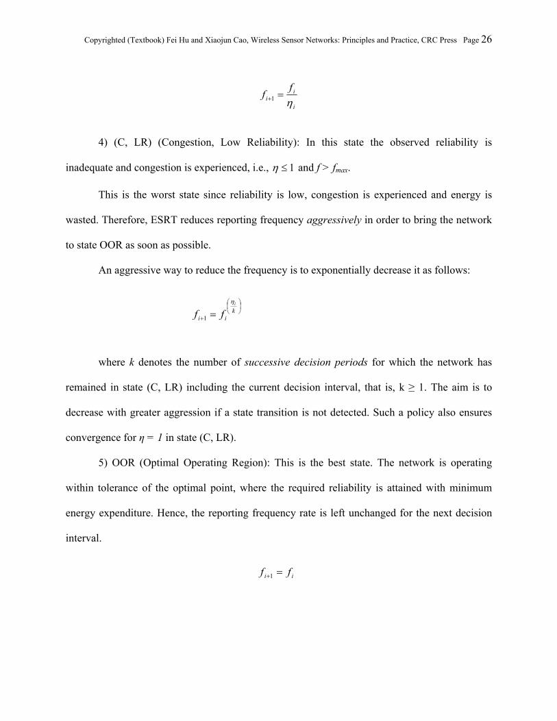
4) (C, LR) (Congestion, Low Reliability): In this state the observed reliability is
inadequate and congestion is experienced, i.e., 1 and f > fmax.
This is the worst state since reliability is low, congestion is experienced and energy is
wasted. Therefore, ESRT reduces reporting frequency aggressively in order to bring the network
to state OOR as soon as possible.
An aggressive way to reduce the frequency is to exponentially decrease it as follows:
kii
i
ff
1
where k denotes the number of successive decision periods for which the network has
remained in state (C, LR) including the current decision interval, that is, k ≥ 1. The aim is to
decrease with greater aggression if a state transition is not detected. Such a policy also ensures
convergence for η = 1 in state (C, LR).
5) OOR (Optimal Operating Region): This is the best state. The network is operating
within tolerance of the optimal point, where the required reliability is attained with minimum
energy expenditure. Hence, the reporting frequency rate is left unchanged for the next decision
interval.
ii ff 1

Copyrighted (Textbook) Fei Hu and Xiaojun Cao, Wireless Sensor Networks: Principles and Practice, CRC Press Page 27
5.3.3 Congestion Detection
Although ESRT’s main purpose is to guarantee an optimized reliability, it also has certain
impacts on network congestion. This can be seen from the above 5 states. On the other hand, to
determine the current network state in ESRT, the sink must be able to detect congestion in the
network. Now the question is, how does a sink know congestion occurs?
Because TCP is not used here, we cannot use traditional approach to determine
congestion levels. Hence, ESRT uses a local buffer level monitoring scheme in individual sensor
nodes to find out congestion event. Any sensor node whose routing buffer overflows due to
excessive incoming packets is said to be congested and it informs the sink of this event. The
details of this mechanism are as follows.
Let bk and bk-1 be the buffer fullness levels at the end of kth and (k-1)th decision intervals,
respectively, and B be the buffer size as in Figure 5.5. For a given sensor node, let Δb be the
buffer length increment observed at the end of last reporting period, i.e.,
– 1
Thus, if the sum of current buffer level at the end of ith reporting interval and the last
experienced buffer length increment exceeds the buffer size, i.e., bk + Δb > B, the sensor node
Good Idea
If you want to slowly approach to a point, you could use “log” or “linear” speed. But if you want to get a fast approaching, “multiplicative” could be a good idea. Of course, “exponential” typically gives us fast enough approaching.

Copyrighted (Textbook) Fei Hu and Xiaojun Cao, Wireless Sensor Networks: Principles and Practice, CRC Press Page 28
infers that it is going to experience congestion in the next reporting interval.
Place Figure 5.5 here.
Figure 5.5 Illustration of buffer level monitoring in sensor nodes [Akan05]
5.4 E2SRT: Enhanced ESRT performance [Sunil08]
Although the above algorithms could make different states go to OOR, however, in
[Sunil08], their simulation results, shown in Figure 5.6, have revealed that when the desired
reliability (R) is set up beyond the capability of current network settings (such as the network’s
sensor deployment strategy, sensor resources, network scale, etc.), the network will never be
able to converge to the OOR state.
Their simulations results also show that the original ESRT scheme (such as the above
described buffer level monitoring scheme) cannot detect this situation by itself. When we use the
original ESRT algorithm to generate a new reporting frequency (for next decision period)
according to this desired reliability value, these values lead the network either to tremendous
congestion or the network operates at a very low frequency rate, thus wasting most of the
bandwidth. As a result, the network oscillates between (congested, low reliability) state and (not
congested, low reliability) state.
Good Idea
Checking node’s local buffer size is a typical way to find out congestion
level. TCP is based on this principle.

Copyrighted (Textbook) Fei Hu and Xiaojun Cao, Wireless Sensor Networks: Principles and Practice, CRC Press Page 29
Place Figure 5.6 here.
Figure 5.6 Normalized reliability fluctuates in ESRT scheme in case of over-demanding desired
reliability requirements.
The actual reliability (r) reached with this oscillation is far below the desired reliability
(R). Apparently, it is also not the maximum reliability we could have obtained with current
network settings. This generally means that the system was running in a very expensive and
inefficient mode: the network is always trying to touch reliability far beyond its capability, which
leads to more congestion, more collision and longer delay. Subsequently, the network throughput
and overall reliability is significantly compromised.
Their extensive simulations [sunil08] show that there is a threshold for this reliability
demand which is decided by current network settings such as network size, radio type,
underlying infrastructures and protocol choices. When the desired reliability is lower than the
threshold, ESRT algorithm can always converge to the OOR mode in several control loops.
However, when this requirement is above the threshold, the network soon falls into oscillation.
When network cannot support desired event reliability, only two network states, i.e., (NC, LR)
and (C, LR), exist (see Figure 5.7).
Place Figure 5.7 here.
Figure 5.7 ESRT protocol state model and transitions when desired reliability is over
demanding.

Copyrighted (Textbook) Fei Hu and Xiaojun Cao, Wireless Sensor Networks: Principles and Practice, CRC Press Page 30
As an example, suppose the desired reliability is 4000 packet successfully received by a
sink in each 10-second interval. However, the network can only handle around 3500 packets per
10 second interval in our simulation settings. Obviously, the reliability requirement is beyond the
network capability, no OOR state exists. ESRT does not take this situation into account, and the
network would fluctuate between (NC, LR) and (C, LR) states.
5.4.1 The Proposed Scheme - E2SRT
Before discussing the solution proposed in [sunil08], which is called the Enhanced Event-
to-Sink Reliability Transport (E2SRT), we formally define the over-demanding desired reliability
problem in ESRT in this section.
The over-demanding desired event reliability problem in E2SRT, denotes a situation
where desired reliability R is sufficiently larger than maxR , so that 1)/( max RR . When the
desired event reliability is over-demanding, we call the network is in OR (Over-demanding
Reliability) state. We shall represent this desired reliability situation as Rod.
We use the following mathematical analysis to demonstrate that when desired event
reliability is over demanding, ESRT will not converge to OOR state, and fluctuates between two
low reliability states (NC, LR) and (C, LR).
Lemma 1: In OR state, the normalized reliability, = r/R, will never fall into the region
of [1- , ).
Proof: Since maxR is the maximum reliability that the network can reach with current
network setting, it follows that observed event reliability, ir maxR . Then,

Copyrighted (Textbook) Fei Hu and Xiaojun Cao, Wireless Sensor Networks: Principles and Practice, CRC Press Page 31
1// max RRRrii
We conclude that )1,0( i .
Lemma 2: In OR state, the network only has two possible working states, namely (NC, LR) and
(C, LR).
Lemma 2 is a straight-forward extension of Lemma 1. However it reveals the most
distinct characteristic of OR state, which is the base for the operations of E^2SRT.
Note that these results are obtained for the situation where the desired reliability is
beyond the capability of sensor network, which implies the following assumptions:
max 1 , maxR
Only two states (NC, LR), (C, LR) are available
Lemma 3: In and only in OR state, starting from iS = (NC, LR), and with linear reliability
behavior when the network is not congested, the network state will transit to 1iS = (C, LR).
Proof: From iS = (NC, LR), ESRT aggressively increments if as follows:
i
ii
ff
1
Hence,
maxmax
1
i
i
i
ii
fff
Since
ii r
Rff max
max and 1/max RR , it follows that:

Copyrighted (Textbook) Fei Hu and Xiaojun Cao, Wireless Sensor Networks: Principles and Practice, CRC Press Page 32
1
1max
maxmax
max
max1 f
R
Rf
R
R
R
rff
fi
i
i
ii
To address this issue, [Sunil08] has divided the problem into the following two sub-
problems:
a. How to detect the over-demanding desired event reliability situation, and
b. If the above situation exists, how to quickly converge to the maximum reliability the
network can reach without requiring the full knowledge of the network conditions.
The major design consideration is how to push the network to approach the Maximum
Reliability Point ( maxf , max ) (MRP) for a given network setting. Similar to ESRT scheme, we
also allow a tolerance zone of width around MRP. If at the end of a decision interval i, the
normalized reliability i is within [ max - , max ] and no congestion is detected in the network,
the network is in Maximum Operating Region (MOR).
Here we follow the definition of tolerance zone of ESRT. It is a protocol parameter
decided by the user requirement. A smaller will generally give greater proximity to MRP
while it may take longer convergence time.
If MRP is known, sink can reduce the desired reliability such that the network can
converge to OOR as in ESRT. However, it is difficult to calculate the exact value of MRP ( maxf ,
max ) due to the following reasons.
Initial deployment,
Nodes move, die or other reasons that will cause the network topology change,
Relocation of events,
Radio interference,

Copyrighted (Textbook) Fei Hu and Xiaojun Cao, Wireless Sensor Networks: Principles and Practice, CRC Press Page 33
Deliberate over demanding to maximize the network throughput.
Consequently, algorithms that assume a priori of constant MOR are not feasible. More
advanced algorithms should be adaptable to the changing network environment. It should be able
to read feedback from sensor network and predict MRP in a recursive manner.
The proposed new algorithm in E2SRT, inherits all the major features of ESRT such as
communication model and network modes definitions. It is sink-based, energy-efficient, and has
fast convergence time. As an enhanced version, E2SRT is more resilient to abrupt network
changes and resource constraints due to its operations in OR states.
In the following section we will describe how E2SRT can approach MOR and how
E2SRT operates in each of the three OR states in details.
In each decision interval, the sink calculates normalized reliability i . In conjunction with
congestion reports, the current network state iS will be determined. Using the decision boundaries
defined in ESRT, with the knowledge of state iS , and the values of if and i , E2SRT will request
the sink to update the event reporting frequency to 1if , and the sink will broadcast the new
frequency value to the sensor nodes. When receiving this updated frequency, the relevant sensor
nodes will report to the sink according to the new frequency in the next decision interval. This
process will repeat until the MOR state is reached. The state transition graph is shown in Figure
5.8.
Place Figure 5.8 here.
Figure 5.8 E2SRT protocol state model and transitions when desired reliability is over
demanding

Copyrighted (Textbook) Fei Hu and Xiaojun Cao, Wireless Sensor Networks: Principles and Practice, CRC Press Page 34
E2SRT introduces a recursive algorithm that converges to MOR in a few rounds of
estimation of MRP. As observed from Figure 5.9, the network shows some linear and symmetry
properties around MOR region in the curve of normalized reliability as a function of reporting
frequency (in logarithm format). And as we previously discussed, the network fluctuates between
only two states (NC, LR) and (C, LR).
Place Figure 5.9 here.
Figure 5.9 Recursive convergence of E2SRT. Starting from (NC, LR)1, the network bouncing in
the cone area of the curve and finally fall into MOR.
Obviously, (NC, LR) is always on left of MRP while (C, LR) is always on right of MRP.
Thus, MRP is always somewhere in between a (NC, LR) state and a (C, LR) state. We will
record the reporting frequency of last (C, LR) state as ),( lrcf , and the frequency of last (NC,
LR) state as ),( lrncf . X-axis of the graph is based on logarithm.
We estimate the frequency for MRP as:
2
loglog
1
),(),(
10lrclrnc ff
if
With the above formula, starting from any of the two states, the network may stay in
either (NC, LR) or (C, LR) for more than one consecutive decision periods. This is because that
the last (NC, LR)/(C, LR) state point is too far apart from MRP compared with last (C, LR)/

Copyrighted (Textbook) Fei Hu and Xiaojun Cao, Wireless Sensor Networks: Principles and Practice, CRC Press Page 35
(NC, LR) state. In case of (C, LR), which means last (C, LR) operating point is too far away
from MRP, we can add a multiplying factor to give more weight on last (NC, LR) operating
point as:
),(),( log1
1log
11 10
lrclrnc fk
fk
k
if
In case of (NC, LR), we have the following formula.
),(),( log1
log1
1
1 10lrclrnc f
k
kf
kif
A detailed description of E2SRT operation in each of the 3 available states is presented
below.
(NC, LR) (No Congestion, Low Reliability): Since the OOR state is not feasible, the goal
of the updating policy is to drive the network to MOR instead of OOR. As pointed out by lemma
3, using ESRT algorithm, the network would inevitably jump into the most undesirable (C, LR)
state. Here we already know that the network is in OR state, as it at least has once jumped to the
(C, LR) state and then fell back into (NC, R) state.
We record the frequency of last (C, LR) state as ),( lrcf , and the frequency of last (NC,
LR) state as ),( lrncf . As observed in basic ESRT scheme, the network would show some linear
and symmetry properties around MOR region in the curve of normalized reliability as a function
of reporting frequency (in logarithm format). This prompts us to update the reporting frequency
as below:
),(),( log1
log1
1
1 10lrclrnc f
k
kf
kif
(C, LR) (Congestion, Low Reliability): In this state, we either detect a transition from
(NC, LR) state (so we know the network is now in OR state), or, we transit from (C, LR) states

Copyrighted (Textbook) Fei Hu and Xiaojun Cao, Wireless Sensor Networks: Principles and Practice, CRC Press Page 36
itself (it means the frequency has to be further reduced). We use a parameter k to count the time
intervals for which the network has successively remained in (C, LR). As k increases, it generally
means ),( lrncf is closer to MOR than ),( lrcf . We therefore assign a higher frequency than ),( lrcf .
Putting together all these considerations, we update the reporting frequency based on the
following formula:
),(),( log1
1log
11 10
lrclrnc fk
fk
k
if
MOR (Maximum Operating Region): In this state, the network is operating within
tolerance of the maximum operating point, where the network is making its best effort to fulfill
the reliability requirement with minimum energy consumption. The reporting frequency remains
unchanged for the next decision interval as:
ii ff 1
The entire E2SRT protocol algorithm is summarized in the pseudo-code in Figure 5.10.
Place Figure 5.10 here.
Figure 5.10 Algorithm of the E2SRT protocol operation
Good Idea
Many students keep asking a same question, “Dr. Who, how do I do some research?” Take a look at this E^2SRT example. It starts from an existing scheme (ESRT), try to find the “hidden” drawbacks or any unsolved issues, and finally think of a good way to overcome those issues. “Improving” is a good way to start your research. But eventually, you need to reach a high-level research – You define an interesting, important research issue by yourself, then use a brand-new way (i.e. other people didn’t find such a way) to solve it! Look at those professors: They are trying to do the same thing – “Find NEW problem, Think of NEW solution.”

Copyrighted (Textbook) Fei Hu and Xiaojun Cao, Wireless Sensor Networks: Principles and Practice, CRC Press Page 37
5.5 CODA: Congestion Detection and Avoidance in Sensor Networks [Wan03]
The above discussed transport schemes have achieved the first goal of WSN transport
layer – reliability. In this section, we discuss a solution to achieve the second goal, i.e.
congestion control.
In order to illustrate the congestion problem, [Wan03] has used simulation results (see
Figure 5.11) to show the impact of congestion on data dissemination in a sensor network for a
moderate number of active sources with varying reporting rates. Its ns-2 simulation assumes the
well-known directed diffusion scheme [CIntanagonwiwat00] operating in a moderately sized 30-
node sensor network using a 2 Mbps IEEE 802.11 MAC with 6 active sources and 3 sinks. Those
6 sensor sources are randomly selected among the 30 nodes in the network and the 3 sinks are
uniformly scattered across the sensor field. Each source generates data event packets at a
common fixed rate.
Place Figure 5.11 here.
Figure 5.11 [Wan03] Total number of packets dropped by the WSN at the sink (Drop Rate) as a
function of the source rate. The x axis is plotted in log scale to highlight data points with low
reporting rates.
Figure 5.11 tells us an interesting conclusion: there exists a water boiling point, that is,
when the source rate increases beyond a certain network capacity threshold (10 events/s in this
network), congestion occurs more frequently and the total number of packets dropped at the sink
increases rapidly. It also shows that congestion could occur even with low to moderate source
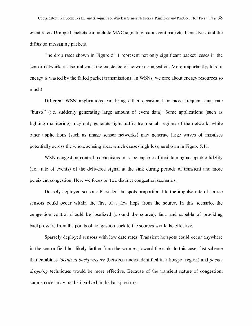
Copyrighted (Textbook) Fei Hu and Xiaojun Cao, Wireless Sensor Networks: Principles and Practice, CRC Press Page 38
event rates. Dropped packets can include MAC signaling, data event packets themselves, and the
diffusion messaging packets.
The drop rates shown in Figure 5.11 represent not only significant packet losses in the
sensor network, it also indicates the existence of network congestion. More importantly, lots of
energy is wasted by the failed packet transmissions! In WSNs, we care about energy resources so
much!
Different WSN applications can bring either occasional or more frequent data rate
“bursts” (i.e. suddenly generating large amount of event data). Some applications (such as
lighting monitoring) may only generate light traffic from small regions of the network; while
other applications (such as image sensor networks) may generate large waves of impulses
potentially across the whole sensing area, which causes high loss, as shown in Figure 5.11.
WSN congestion control mechanisms must be capable of maintaining acceptable fidelity
(i.e., rate of events) of the delivered signal at the sink during periods of transient and more
persistent congestion. Here we focus on two distinct congestion scenarios:
Densely deployed sensors: Persistent hotspots proportional to the impulse rate of source
sensors could occur within the first of a few hops from the source. In this scenario, the
congestion control should be localized (around the source), fast, and capable of providing
backpressure from the points of congestion back to the sources would be effective.
Sparsely deployed sensors with low date rates: Transient hotspots could occur anywhere
in the sensor field but likely farther from the sources, toward the sink. In this case, fast scheme
that combines localized backpressure (between nodes identified in a hotspot region) and packet
dropping techniques would be more effective. Because of the transient nature of congestion,
source nodes may not be involved in the backpressure.
Copyrighted (Textbook) Fei Hu and Xiaojun Cao, Wireless Sensor Networks: Principles and Practice, CRC Press Page 39
Sparsely deployed sensors generating high data-rate events: In this scenario, both
transient and persistent hotspots are distributed throughout the sensor field. To control
congestion, we need a fast scheme to resolve localized transient hotspots, and to perform closed-
loop rate regulation of all source nodes that contribute toward creating persistent hotspots.
[Wan03] proposed an energy efficient congestion control scheme for sensor networks
called CODA (Congestion Detection and Avoidance) that comprises three mechanisms:
• Congestion detection. The first step towards congestion control is to accurately and
efficiently detect congestion. That is, we need to find out whether congestion occurs in the
network or not. If it does, where is it? Congestion detection is based on the observations by each
sensor: what are the present and past communication channel traffic conditions in the current
sensor? What is the current buffer occupancy in the sensor? We must know the state of the
communication channel because neighboring sensors may simultaneously use such a channel to
transmit data. However, we cannot persistently listen to the channel to measure local loading
since it could cause high energy costs. Therefore, CODA uses a sampling scheme that only
activates local channel monitoring in a certain time. Once congestion is detected, nodes signal
their upstream neighbors via a backpressure mechanism.
• Open-loop, hop-by-hop backpressure. If a node detects congestion, it propagates
backpressure signals one-hop upstream toward the source. If a node receives backpressure
signals, it throttles its sending rates, or it may drop packets based on the local congestion policy
(e.g., packet drop, AIMD, etc.). When an upstream node (toward the source) receives a
backpressure message, it checks its own local network conditions. If it also detects congestion, it
will further propagate the backpressure upstream.
• Closed-loop, multi-source regulation. Closed-loop rate regulation operates over a

Copyrighted (Textbook) Fei Hu and Xiaojun Cao, Wireless Sensor Networks: Principles and Practice, CRC Press Page 40
slower time scale than the above open-loop control. But it is capable of asserting congestion
control over multiple source nodes from a single sink in the event of persistent congestion. Each
source node compares its data rate to some fraction of the maximum theoretical throughput of
the channel (details in [Wan03]). If its data rate is less than such throughput, it simply regulates
its rate. However, when its rate is higher than the throughput, it could have a contribution to
network congestion. Under this circumstance the closed-loop congestion control is triggered.
And the source enters sink regulation, i.e., it uses feedback (e.g., ACK) from the sink to maintain
its rate. The reception of ACKs in a source node serves as a self-clocking mechanism to help the
source to maintain its current event rate. However, if a source fails to receive ACKs, it will force
itself to reduce its own rate.
The relationship between open-loop and closed-loop control is as follows: Because
hotspots (i.e. congestion locations) can occur in different regions of a sensor field due to the
above different scenarios, CODA needs both open-loop hop-by-hop backpressure and closed-
loop multi-source regulation mechanisms. These two control mechanisms can be used separately.
But it is more efficient to make them complement each other nicely.
From the above description we can also see that rate control scheme has different
operations in source nodes, the sink, or intermediate nodes. Sources know the properties of the
sending traffic while intermediate nodes do not. A sink has best understanding of the fidelity rate
for the received signal, and in some applications, sinks are powerful nodes that are capable of
performing complicated heuristics. The goal of CODA is to do nothing during no-congestion
conditions, but be responsive enough to quickly mitigate congestion around hotspots once
congestion is detected.

Copyrighted (Textbook) Fei Hu and Xiaojun Cao, Wireless Sensor Networks: Principles and Practice, CRC Press Page 41
5.5.1 Open-Loop Hop-by-Hop Backpressure
The above discussions have briefly described fast /slow time-scale congestion control.
Backpressure belongs to fast time-scale control mechanism. If a sensor detects congestion, it
broadcasts a suppression message to its 1-hop upstream neighbors. It knows where the upstream
nodes are by checking the routing protocol, which is located below the transport layer protocol in
WSN protocol stack.
When an upstream node (toward the source) receives a backpressure message, a node
may keep propagating backpressure signals if it finds serious congestion. But it may not send
back backpressure signal, and just simply drops its incoming data packets upon receiving a
backpressure message to prevent its queue from building up.
The above discussion is for open-loop control. For closed-loop congestion control, it
requires to deal with any persistent congestion locally instead of propagating the backpressure
signal.
CODA defines depth of congestion as the number of hops that the backpressure message
has traversed before a non-congested node is encountered. The depth of congestion can be used
Good Idea
Open-loop and close-loop control: They have been used in many system control applications. Open-loop control is simpler and easier to implement. But close-loop uses output feedback to adjust the input, which typically brings more accurate, stable system control.

Copyrighted (Textbook) Fei Hu and Xiaojun Cao, Wireless Sensor Networks: Principles and Practice, CRC Press Page 42
by the routing protocol as follows:
Selecting better route path: If the depth of congestion is too high, a routing protocol may
give up the current path and finds new one. This can reduce traffic over the paths suffering deep
congestion.
Intentionally drop command messages to reduce congestion: The nodes can silently
suppress or drop important signaling (i.e. command) messages associated with routing or data
dissemination protocols. Such actions would help to push data flows out of congested regions
and away from hotspots in a more transparent way.
5.5.2 Congestion Detection
To detect congestion, we have some easy ways such as checking if a queue in the sensor
is full or not, or measuring the current communication channel traffic load – if the load is
approaching the upper bound, it is an indication of congestion.
The first detection approach, monitoring queue size, has low execution overhead. But it
may not provide accurate congestion detection since the queue can overflow due to many local
conditions. The second approach, listening to the communication channel shared among
neighbors, can tell us the channel loading or even give us protocol signaling information on
collision detection effect. Therefore, we prefer the second approach. However, because listening
to channels continuously can bring high energy cost, we should use it only at appropriate time in
order to minimize system cost.
So, what is the good time to activate the channel monitoring? Let’s utilize a trick in MAC
(Medium Access Control) protocols. As we know, typically a sensor listens to the channels

Copyrighted (Textbook) Fei Hu and Xiaojun Cao, Wireless Sensor Networks: Principles and Practice, CRC Press Page 43
before sending packets. Such a channel listening procedure is called “carrier sense” in MAC
protocols. If the channel is clear during this period, then the radio switches into the transmission
mode and sends out a packet.
Therefore, the best time to perform channel monitoring is when “carrier sense” occurs.
This is because there will be no extra cost to listen and measure channel loading when a node
wants to transmit a packet since carrier sense is required anyway before a packet transmission.
In Figure 5.12 we can see a typical scenario with hotspots or congestion areas. In this
example, nodes 1 sends data to node 3; and node 4 sends data to node 5. Two data flows both
pass through node 2.
As we can see from the “channel load” of Figure 5.12, node 2 has high buffer occupancy.
Then node 2 activates the channel loading measurement. The channel loading measurement will
stop naturally when the buffer is cleared, which indicates with high probability that any
congestion is mitigated and data flows smoothly around the neighborhood.
Place Figure 5.12 here.
Figure 5.12 A simple IEEE 802.11 wireless network of 5 nodes to illustrate receiver-based
congestion detection. [Wan03]
5.5.3 Listening to channel based on sampling
Let’s define an epoch time as a time period of transmitting multiple packets. When a node
listens to the channel, we require it to listen for at least 1 epoch time to measure the channel load.
During an epoch period, if a node continuously listens to the channel, it would take lots of

Copyrighted (Textbook) Fei Hu and Xiaojun Cao, Wireless Sensor Networks: Principles and Practice, CRC Press Page 44
energy cost. Therefore, CODA only performs periodic sampling (i.e. listening to channel once
for a while) so that the radio can be turned off if not sampling.
We use a simple sampling scheme as follows: We measure the channel load for N
consecutive epoch times of length E. In each epoch time, we use a predefined sampling rate to
obtain channel state information. That is, we try to get the number of times that the channel state
is busy or idle within a single sensing epoch.
We then calculate the sensed channel load Φ as the exponential average of Φn (the
measured channel load during epoch n) with parameter α (0<α<1) over the previous N
consecutive sensing epochs, as shown in the equation below.
)},,,2,1{(,)1( 111 Nnnnn
If the send buffer is cleared before n counts to N, then the average value is ignored and n
is reset to 1. Note: The tuple (N,E,α) offers a way to tune the sampling scheme to accurately
measure the channel load for specific radio and system architectures.
Based on the above equation, we obtain the time-varied sensed channel load. When such
a load exceeds a threshold, it means network congestion. In this case, a node broadcasts a
suppression message as a backpressure signal and at the same time exercises the local congestion
policy. A node will continue broadcasting this message up to certain maximum number of times
with minimum separation as long as congestion persists.
The suppression message provides the basis for the open-loop backpressure mechanism.

Copyrighted (Textbook) Fei Hu and Xiaojun Cao, Wireless Sensor Networks: Principles and Practice, CRC Press Page 45
5.6 STCP: A Generic Transport Layer Protocol for WSN [YIyer05]
STCP [YIyer05] provides a generic, scalable and reliable transport layer paradigm for
sensor networks. The WSN base-station implements the majority of STCP functionalities since it
has unlimited resources compared to sensors.
5.6.1 Data transmission sequence in STCP
Similar to the principle of TCP 3-way handshake protocol that aims to establish an end-
to-end TCP connection, before transmitting packets, a sensor node establishes an association
(similar to TCP’s connection concept) with the base station via a Session Initiation Packet.
The session initiation packet tells the base station the following information: the number
of flows originating from the node, the type of data flow, transmission rate and required
reliability. When the base station receives the session initiation packet, it stores all the
information, sets the timers and other parameters for each flow, and acknowledges this packet.
Such an acknowledgement (ACK) packet is important for the sensor node to ensure that
the association is established. After a node receives the ACK from the base-station, it can now
start transmitting data packets to the base station. In the reverse path, the base station transmits
an ACK or NACK (negative ACK) depending on the type of data flow.
5.6.2. STCP Packet formats
Figure 5.13 shows the format of a session initiation packet. A source node transmits
packets associated with each data flow independently, since the transmission characteristics may

Copyrighted (Textbook) Fei Hu and Xiaojun Cao, Wireless Sensor Networks: Principles and Practice, CRC Press Page 46
be different in different flows. In Figure 5.13, the first field is the sequence number (16 bits
long). It is set to zero for the session initiation packet. The second field (Flows, 8 bits long)
indicates the number of flows originating at the node. The “clock” field has the local clock value
at the time of transmission. Flow Id is used to differentiate packets from different flows. The
Flow Bit field specifies whether the flow is continuous (i.e. the data flow doesn’t stop) or event-
driven (i.e. only sends out packets when an event is detected). For continuous flows, the
Transmission rate field indicates the rate at which a packet will be transmitted by the source
node.
The Reliability field directly relates to WSN transport layer tasks. Again, it means the
packet arrival success rate. Here, this field gives the expected reliability required by the flow.
Place Figure 5.13 here.
Figure 5.13 Session Initiation Packet [YIyer05]
STCP data packet header is shown in Figure 5.14. It is similar to session initiation packet
header. The Sequence number for a data packet is a non-zero positive integer (for session
initiation packet, it is zero). The Flow Id indicates the flow type which helps the base station
identify the characteristics of the packet for that node.
The packet header includes an important field that relates to congestion control, called
Congestion Notification (CN). As 1-bit field, when it is 1, it means congestion occurs. The Clock
field gives the local time at which the packet was transmitted. The base station uses the clock
value to calculate the Estimated Trip Time (ETT) for that node and flow Id.
Place Figure 5.14 here.

Copyrighted (Textbook) Fei Hu and Xiaojun Cao, Wireless Sensor Networks: Principles and Practice, CRC Press Page 47
Figure 5.14 STCP Data Packet Header
The ACK packet format is shown in Figure 5.15. All fields are as explained before. The
ACK / NACK field tells that it is a positive or negative acknowledgement. STCP uses the 32-bit
clock field in conjunction with the sequence number field to avoid issues related to wrap-around.
The Options field is for future extension purposes.
Place Figure 5.15 here.
Figure 5.15 STCP Acknowledgement Packet
5.6.3 Continuous Flows
This section focuses on “continuous flows” case. Next section is about “event-based
flow” case. Note that the base station can use session initiation packet to get to know the sending
rate of the source. Thus it can estimate the expected arrival time for the next packet. The base
station maintains a timer and sends a negative acknowledgement (NACK) if it does not receive a
On packet format: When you design a network protocol, you should know the packet format first. This is because protocol operations are different when the field content in a packet header is different. Sometimes we don’t have standardized packet format to use. For this case, you need to define packet format by yourself. Try to minimize the field length – If you could use 3 bits to cover 5 cases, why should you use 4 bits in that field?

Copyrighted (Textbook) Fei Hu and Xiaojun Cao, Wireless Sensor Networks: Principles and Practice, CRC Press Page 48
packet within the expected time.
When the base station receives a packet from a sensor node, it calculates the Estimated
trip time (ETT) for the next packet to reach the base station by one of the following methods:
1) It can calculate the Timeout value by using the expression (T + α × ETT), where T is
the time between two successive transmissions, and alpha (α) is a positive integer that varies
with ETT. In this approach, the base station constantly checks to see if it has received a packet
within (T + α × ETT) time units for each sensor node. If a packet has been received within time,
it decreases alpha (α) by 0.5. If a packet is lost (i.e. timeout occurs), or if the base station
receives a packet after transmitting a NACK for it, it increases alpha (α) by 0.5.
2) The second approach is to use Jacobson/Karels algorithm [VJacobson88] which
considers the variance of the round trip time (RTT). Here we use ETT instead of RTT. In this
approach, we can modify Jacobson/Karels algorithm by considering ETT. The base station
dynamically varies the values of delta (δ), mu (μ) and phi ( ) in the following expressions:
| |
μ
When a NACK is received, a source node retransmits packets. If the source node does not
receive a NACK, the packet must have reached the base station, unless the NACK is lost.
Therefore, the base station maintains a record of all packets for which it has sent a NACK.
If a packet that has been NACKed successfully arrives, the base station clears the
corresponding entry from the record. The base station periodically checks this record and, if it

Copyrighted (Textbook) Fei Hu and Xiaojun Cao, Wireless Sensor Networks: Principles and Practice, CRC Press Page 49
finds an entry, retransmits a NACK.
5.6.4 Event-driven Flows
The previous case used NACK since it was for “continuous” flow. We assume that not
many packets are lost, thus NACK is sent back occasionally. If we used ACK (positive
acknowledgment) in that case, we would have too many ACKs since continuous data flow have
lots of traffic.
In this section we move to “event-driven” flows. In this case, the flow data is much less
than the former case since the data transmission is triggered only when a new event occurs. The
positive acknowledgements (ACK) are used to let a source node know if a packet has reached the
base station. Because the data is received occasionally, there could be big gaps between two
packet arrivals. Thus the base station cannot estimate arrival times of next data packet.
Similar to TCP principle, the source node buffers each transmitted packet and also
invokes a timer. When an ACK is received, the corresponding packet is deleted from the buffer.
When the timer fires before an ACK is received, packets in the buffer are assumed to be lost and
are retransmitted.
5.6.5 Reliability
We mentioned before that a sensor node can specify the required reliability for each flow
in the session initiation packet. For continuous flows, the base station calculates a running
average of the reliability. Reliability is measured as the percentage of packets successfully

Copyrighted (Textbook) Fei Hu and Xiaojun Cao, Wireless Sensor Networks: Principles and Practice, CRC Press Page 50
received. Note that the base station will not send a NACK if the current reliability satisfies the
required reliability. The base station transmits NACKs only when the reliability goes below the
required level.
5.6.6 Congestion Detection and Avoidance
How does STCP achieve the final goal - congestion detection and avoidance? We may
refer to some of traditional schemes. The random early detection (RED) mechanism designed by
Floyd and Jacobson [SFloyd93] proposes that an intermediate node drop a packet when it
experiences congestion. The source is, therefore, effectively notified by a subsequent timeout or
a NACK. Since dropping of packets is detrimental to sensor networks, STCP doesn’t adopt this
approach.
In the scheme proposed in DECbit [KRamakrishnan90], intermediate nodes monitor the
traffic load and explicitly notify the end nodes by setting a binary congestion bit in the packets.
STCP adopts this method of explicit congestion notification with some modification.
Each STCP data packet has a congestion notification bit in its header. Every sensor node
maintains two thresholds in its buffer: thlower and thhigher. When the buffer reaches thlower, the
congestion bit is set with a certain probability. The value of this probability can be determined
by an approach similar to that employed in RED. When the buffer reaches thhigher, that means the
congestion is serious, then the node will set the congestion notification bit in every packet it
forwards.
After receiving this packet with congestion notification field, the base station informs the
source of the congested path by setting the congestion bit in the ACK packet. When receiving the

Copyrighted (Textbook) Fei Hu and Xiaojun Cao, Wireless Sensor Networks: Principles and Practice, CRC Press Page 51
congestion notification, the source will either route successive packets along a different path or
slow down the transmission rate. Note that the nodes rely on the routing layer algorithm to find
alternate routes.
5.6.7 Data-centric Applications
In data-centric applications, we typically are only interested in collective network-wide
information instead of individual sensor node’s data. A few examples are monitoring of seismic
activity, finding maximum temperature in the network, etc. In such applications, the intermediate
nodes may aggregate the correlated data as part of the data aggregation process.
Due to data aggregation from large number of source nodes, we shouldn’t ask a base
station to acknowledge all the source nodes by an ACK or NACK because doing that can deplete
network resources and energy.
Hence, for data-centric applications, STCP does not provide any acknowledgement
scheme. This is similar to UDP case in Internet. STCP assumes that data from different sensors
are correlated and loss tolerant to the extent that events are collectively and reliably sent to the
base station. This view is supported by the authors in ESRT.
5.7 GARUDA: Achieving Effective Reliability for Downstream Communication [Seung-
Jong08]
ESRT takes care of event-to-sink (upstream) reliability issues. In this section, we
consider the problem of reliable downstream point-to-multipoint data delivery, from a sink to

Copyrighted (Textbook) Fei Hu and Xiaojun Cao, Wireless Sensor Networks: Principles and Practice, CRC Press Page 52
multiple sensors. Especially we will discuss GARUDA (a mythological bird that reliably
transported gods) proposed in [Seung-Jong08] which can efficiently achieve such a downstream
reliability.
Since a sink typically sends out important data (such as data query commands) to sensors,
we require that any message from the sink has to reach the sensors reliably. Consider an image
sensor network application. The sink may send one of the following three classes of messages,
all of which have to be delivered reliably to the sensors: 1) Over-the-air programming codes: If
the underlying network is composed of reconfigurable sensors that can be reprogrammed, the
sink may want to send a particular (say, upgraded) image detection/processing software to the
sensors. We refer to such messages as the control code. 2) Data query data: Next step, the sink
may have to send a database of target images to the sensors to help in the image recognition
triggered by subsequent queries. We refer to such data as the query-data. 3) Data collection
commands: Finally, the sink may send out one or more queries requesting information about the
detection of a particular target. The sensors can then match targets detected with the pre-stored
images and respond accordingly.
5.7.1 Challenges to the Downstream Reliability of WSN
A. Environment Constraints
To implement downstream reliability, we need to overcome some challenges. One of
them is to consider the limited network bandwidth and energy sources in a WSN. We need to
minimize the number of retransmission overheads to ensure reliability because by doing so can
reduce both bandwidth and energy consumption of the message overheads in the reliability

Copyrighted (Textbook) Fei Hu and Xiaojun Cao, Wireless Sensor Networks: Principles and Practice, CRC Press Page 53
process.
We should also realize that node failures (due to power draining) lead to dynamic
network topology. The downstream reliability should be adaptive to such a dynamic topology,
that is, it cannot use statically constructed mechanism (say, a broadcast tree) that do not account
for the dynamics of the network.
Another challenge comes from the scale of the sensor network. A WSN can be expected
to be of a large scale in terms of the number of nodes and, hence, the diameter of the network.
This means that there is a tremendous amount of spatial reuse possible in the network that should
be tapped for achieving the best capacity and, hence, delay. However, the specific loss recovery
mechanism used may severely limit such spatial reuse as we elaborate later.
B. Acknowledgment (ACK)/NACK Paradox
Should a receiver use an ACK or NACK to tell the sender the packet arrival situation?
This depends on different conditions. For instance, if the packet loss rate is very low, NACK-
based approach can save more bandwidth since there will be few NACKs sent back to the
sender. But for high packet loss environment, ACK-based approach can save more message
overhead.
In addition, if we use NACK-based approach, we need to handle the last-pack-loss issue.
This was visited before. The NACK-based loss recovery scheme will inherently require in-
sequence forwarding of data by nodes in the network to prevent a NACK implosion [CYWan02].
This will clearly limit the spatial reuse achieved in the network.

Copyrighted (Textbook) Fei Hu and Xiaojun Cao, Wireless Sensor Networks: Principles and Practice, CRC Press Page 54
C. Reliability Semantics
In WSNs we need to consider sensor data location dependency and redundancy.
Location dependency: In many cases, we need to find where the event is exactly located.
A data query command (sent from a base-station) can be location dependent such as “Send
temperature readings from rooms X, Y, and Z.”
Location redundancy: Due to large sensor density in most WSN applications, it is not
necessary for all sensors in the same event area to reliably deliver their locally sensed data to the
sink. Such upstream (event-to-sink) “partial reliability” can save network bandwidth. GARUDA
is a downstream (sink-to-event) reliability scheme, which also uses “partial reliability”, that is,
the sink only guarantees reliable communications with part of the sensors in a neighborhood
area.
GARUDA defines the “reliability semantics” that are required in WSN based on the
above characteristics. It classifies the reliability semantics into four categories:
1. Delivery to the entire field (i.e. whole WSN), which is the default semantics,
2. Delivery to sensors in a sub-region of the field, which is representative of location-
based delivery,
3. Delivery to sensors such that the entire sensing field is covered, which is representative
of redundancy-aware delivery, and
4. Delivery to a probabilistic subset of sensors, which corresponds to applications that
perform resolution scoping.
Figures 5.16 (a), (b), (c), and (d) illustrate categories 1 through 4, respectively.
Place Figure 5.16 here.

Copyrighted (Textbook) Fei Hu and Xiaojun Cao, Wireless Sensor Networks: Principles and Practice, CRC Press Page 55
Figure 5.16 Types of reliability semantics. (a) Reliable delivery to all sensors.(b) Reliable
delivery to a sub-region. (c) Reliable delivery to minimal sensors to cover the sensing field. (d)
Probabilistic reliable delivery to 80 percent of the sensors. [Seung-Jong08]
5.7.2 GARUDA Design Basics
Let’s first take an overview of GARUDA’s design. The centerpiece of GARUDA’s
design is an instantaneously constructible loss recovery infrastructure called the core. The core
can be seen as an approximation of the minimum dominating set (MDS) of the network topology.
The dominating set is a set of nodes through which we could reach all other nodes easily (such as
using at most 1-hop communication from one of the dominant set nodes).
MDS is not a new concept to solve networking problems [RSivakumar99]. But
GARUDA makes a new contribution on establishing an optimal core for the loss recovery
process. It constructs the core during the course of a single packet flood, and uses a two-phase
loss recovery strategy. Its loss recovery uses out-of-sequence forwarding and is tailored to satisfy
the goal of minimizing the retransmission overheads and the delay. It also uses a candidacy-
based approach for the core construction to support multiple reliability semantics (Figure 5.16).
GARUDA is a pulsing-based approach, which means that it can deliver a single packet
reliably to all network nodes. It can ensure the reliable delivery of the first packet of messages of
any size. It has the advantages of NACK-based schemes but, at the same time, avoids any pitfalls
that consequently arise.
In the following GARUDA overview, we discuss its core infrastructure based on the
assumption that the first packet is reliably delivered. Then, we see how it can achieve reliable

Copyrighted (Textbook) Fei Hu and Xiaojun Cao, Wireless Sensor Networks: Principles and Practice, CRC Press Page 56
delivery of the first packet.
A. Loss Recovery Servers: Core
GARUDA calls its core as a set of local designated loss recovery servers (here servers are
not machines; they simply refer to nodes providing loss recovery services). We need to solve two
problems when using an algorithm to construct such a core: (1) how does the algorithm choose
the core nodes for the purpose of minimizing the retransmission overheads? 2) how does the core
construction algorithm adapt to the dynamic network topology change due to node failures (or
other reasons)?
Believe it or not, GARUDA finishes the core construction during the first packet
delivery. As long as the first packet is reliably delivered, we could determine the hop_count of
each node, which is the distance of a node from the sink. Any node with a hop_count that is a
multiple of three (such as 3, 6, 9, etc.) will elect itself as a core node if it has not heard from any
other core nodes. The reason we select a node at 3i hop distance as a core node is because it can
cover the other nodes at 3i + 1 or 3i - 1 hop distances so that it can behave like as one of the
MDS in the direction from a sink to sensors.
In summary, the instantaneous construction of the core nodes during the first packet
delivery of every new message, efficiently addresses any vulnerability in the network in terms of
node failures.
B Loss Recovery Process

Copyrighted (Textbook) Fei Hu and Xiaojun Cao, Wireless Sensor Networks: Principles and Practice, CRC Press Page 57
B.1 Out-of-Sequence Packet Forwarding
In traditional transport protocol such as TCP in Internet, we deliver all packets with in-
order sequence IDs. That is, a sender will not move to higher sequence IDs if lower ones are not
ACKed by the receiver side. Sometimes the network can lose a packet. Then we need to
retransmit those lost packets before we send packets with higher sequence IDs. The main
drawback of the in-sequence forwarding strategy is that precious downstream (sink-to-event)
network resources can be left underutilized when the forwarding of higher sequence number
packets is suppressed in the event of a loss.
Therefore, GARUDA uses out-of-sequence packet forwarding strategy which can
overcome the above drawback since nodes that have lost a packet can continue to forward any
higher (or lower) sequence number packets.
B.2 Two-Stage Loss Recovery
Once the core is constructed, a two-stage loss recovery is used: (1) The core nodes
recover all lost packets; (2) then the non-core nodes recover the lost packets.
Because we only select nodes with hop-count of 3i as core nodes, the number of non-core
nodes will be a substantial portion of the total number of nodes in the network. Therefore we ask
core nodes to recover those lost packets first, which can preclude any contention from lots of
non-core nodes.
The second phase of the loss recovery will not start until when a non-core node overhears
a message from the core node indicating that it has received all the packets. Hence, the second

Copyrighted (Textbook) Fei Hu and Xiaojun Cao, Wireless Sensor Networks: Principles and Practice, CRC Press Page 58
phase does not overlap with the first phase in each local area, preventing any contention with the
first phase recovery.
5.7.3 GARUDA Framework
To see more details on GARUDA scheme, let’s assume a network topology as shown in
Figure 5.17. As mentioned before, the first-packet delivery procedure can find core nodes with
hop_count of 3i. We call all nodes with the same hop_count from the sink as a “band”. The
band-ID is the same as hop_count.
We consider all nodes with the same band-ID (i.e. in the same “band”). Obviously the
bands can be viewed as concentric circles around the sink. Moreover, every core node should
have a band_ID of 3, 6, 9, etc.
Place Figure 5.17 here.
Figure 5.17 Instantaneous core construction in GARUDA. [Seung-Jong08]
A. Core Construction Procedure
In the sink:
When the sink sends the first packet, it stamps the packet with a “band-ID” (bId)
of 0. When a node receives the first packet, it increments its bId by 1 and sets the
resulting value as its own band-ID.

Copyrighted (Textbook) Fei Hu and Xiaojun Cao, Wireless Sensor Networks: Principles and Practice, CRC Press Page 59
In the nodes in 3i bands:
Those nodes are allowed to elect themselves as core nodes. When a node with a
band-ID 3i forwards the packet (after a random waiting delay from the time it received
the packet), it will first see if it has heard from any other core node in the same band. If it
hasn’t heard of any other nodes that claim themselves as core nodes, it will claim itself as
core nodes. The reason of doing this is to reduce the communication conflict between any
two core nodes (and thus minimize the number of core nodes).
If any node in the core band (3i) has not selected itself to be a core yet, and when
it receives a core solicitation message explicitly, it chooses itself as a core node at that
stage.
To keep band-to-band communications, every core node in the 3(i+1) band should
also know of at least one core node in the (3i) band. If it receives the first packet through
a core node in the (3i) band, it can determine this information implicitly as every packet
carries the previously visited core node’s identifier bId.
Nodes in 3i + 1 bands:
When a node A with a band-ID (3i + 1) receives the first packet, it checks to see if
the packet arrived from a core node or from a non-core node. If the source S0 was a core
node, node A sets its core node as S0. Otherwise, it sets S0 as a candidate core node and
starts a core election timer that is set to a value larger than the retransmission timer for
the first-packet delivery. If S1 hears from a core node '0S before the core election timer
expires, it sets its core node to '0S .
However, if the core election timer expires before hearing from any other core

Copyrighted (Textbook) Fei Hu and Xiaojun Cao, Wireless Sensor Networks: Principles and Practice, CRC Press Page 60
node, it sets S0 as its core node and sends a one-to-one (unicast) message to S0 informing
it of the decision.
Nodes in 3i + 2 bands:
When a node A with a band-ID of the form (3i + 2) receives the first packet, it
cannot (at that point) know of any 3(i+1) node. Hence, it forwards the packet without
choosing its core node but starts its core election timer. If it hears from a core node in the
3(i+1) band before the timer expires, it chooses that core node as its core node. If A does
not hear from any node in the 3(i+1) band, it sends an anycast core solicitation message
with only the target band-ID set to 3(i+1). Any node in the 3(i+1) band that receives the
anycast message is allowed to respond after a random waiting delay. The delay is set to a
smaller value for core nodes to facilitate the reuse of an already elected core node.
B. Two-Phase Loss Recovery
a. Loss detection. When a core node receives an out-of-sequence packet, the core node
infers a loss, and it sends a request to an upstream (closer to the sink) core node only if it is
notified that the missing packet is available at the upstream core node.
b. Loss recovery. When a core node receives a request from a downstream core node, it
performs a retransmission for the lost packet. Figure 5.18 shows the loss detection and the loss
recovery between core nodes at the (3i) band and core nodes at the 3(i+1) band. If any of the
non-core nodes overhears the requested packet, it retransmits the requested packet.

Copyrighted (Textbook) Fei Hu and Xiaojun Cao, Wireless Sensor Networks: Principles and Practice, CRC Press Page 61
Place Figure 5.18 here.
Figure 5.18 Loss recovery for core nodes in GARUDA. [Seung-Jong08]
Good Idea
GARUDA uses “bands” to define WSN core and non-core nodes. This is an interesting idea. A researcher has used “throwing a stone in water” phenomenon to find an interesting way to define network topology – “ripples”. That is, he tries to generate “ripples” when a sender broadcasts a message. The “ripple” concept is similar to the “band” concept here. But how to define the band/ripple generation procedure is not an easy task since we need to consider many details such as broadcasting time, hop count, neighbors’ communication conflicts, etc.

Copyrighted (Textbook) Fei Hu and Xiaojun Cao, Wireless Sensor Networks: Principles and Practice, CRC Press Page 62
Problems & Exercises
5.1 Multi-choice questions:
(1) Which of the following does NOT belong to the tasks of Transport layer?
A. Reliable source-to-destination transmission.
B. Network Congestion Detection.
C. Network Congestion Avoidance.
D. Buffer Management.
(2) Why does TCP NOT work in WSN?
A. TCP has too much overhead when used in sensors.
B. The errors accumulate in each wireless hop.
C. TCP needs large power consumption.
D. Both A and B.
(3)Which of the following does NOT belong to PSFQ’s features?
A. Send out data slowly;
B. Recover data quickly;
C. Hop-to-hop error recovery.
D. All of the above.

Copyrighted (Textbook) Fei Hu and Xiaojun Cao, Wireless Sensor Networks: Principles and Practice, CRC Press Page 63
(4) If a single hop has wireless loss rate 10%, 5-hop links will bring loss rate of :
A. 50%
B. 5%
C. 10-5
D. 0.2
(5)PSFQ protocol does NOT have which of the following functions?
A. Data Pump;
B. Error-recovery (fetch);
C. End-to-end retransmission and timer setup.
D. Status reporting.
(6) ESRT does NOT have which of the following features?
A. It can achieve sink-to-sensors reliability.
B. It adjusts the sensor’s reporting frequency based on reliability requirement.
C. It aims to reach OOR status.
D. If in (Congestion, Low Reliability), it needs to quickly decrease reporting
frequency.

Copyrighted (Textbook) Fei Hu and Xiaojun Cao, Wireless Sensor Networks: Principles and Practice, CRC Press Page 64
(7) E2SRT improves ESRT from which of the following aspect(s)?
A. When the desired reliability is beyond the capability of current network settings, the
network will never be able to converge to the OOR state where normalized
reliability equals to 1.
B. The network oscillates between congested low reliability state (C, LR) with fairly
high reporting rate to the state of not congested low reliability state (NC, LR) with
very low reporting rate.
C. It greatly saves sending power consumption during OOR approaching.
D. Both A and B.
(8) CODA has which of the following features?
A. CODA is to achieve reliability.
B. CODA achieves congestion reduction.
C. CODA achieves both reliability and congestion avoidance.
D. None of the above.
(9) STCP does NOT have which of the following features?
A. STCP protocols are implemented in the sensor nodes.
B. STCP is a generic, scalable and reliable transport layer paradigm for WSN.
C. STCP provides both reliability and congestion control.

Copyrighted (Textbook) Fei Hu and Xiaojun Cao, Wireless Sensor Networks: Principles and Practice, CRC Press Page 65
D. STCP protocols mostly run in base station.
(10) GARUDA has which of the following procedure(s)?
A. It achieves reliable sink to sensors transmission.
B. It uses the concept of dominant set to build the core.
C. It recovers data in different ways for core and non-core nodes.
D. All of the above.
5.2 Explain why TCP does NOT work well in WSN.
5.3 Explain how PSFQ set up retransmission timer in each node for packet loss case.
5.4 Why does ESRT propose the concept of states and use OOR as the aim?
5.5 Besides the formula ESRT uses when approaching to OOR, can you think of other good
functions that can also achieve the similar approaching speed?
5.6 How does ESRT detect congestion?
5.7 How does E2SRT improve ESRT?
5.8 Explain how GARUDA form the core nodes.