Chapter 5: Thermal Properties of Crystal Lattices

Debye

January 30, 2017

Contents

1 Formalism 2

1.1 The Virial Theorem . . . . . . . . . . . . . . . . . . . . . . . . . . . . 2

1.2 The Phonon Density of States . . . . . . . . . . . . . . . . . . . . . . 5

2 Models of Lattice Dispersion 7

2.1 The Debye Model . . . . . . . . . . . . . . . . . . . . . . . . . . . . . 7

2.2 The Einstein Model . . . . . . . . . . . . . . . . . . . . . . . . . . . . 9

3 Thermodynamics of Crystal Lattices 9

3.1 Mermin-Wagner Theory, Long-Range Order . . . . . . . . . . . . . . 10

3.2 Thermodynamics . . . . . . . . . . . . . . . . . . . . . . . . . . . . . 12

3.3 Thermal Expansion, the Gruneisen Parameter . . . . . . . . . . . . . 14

3.4 Thermal Conductivity . . . . . . . . . . . . . . . . . . . . . . . . . . 18

1

In the previous chapter, we have shown that the motion of a harmonic crystal can

be described by a set of decoupled harmonic oscillators.

H =1

2

∑k,s

|Ps(k)|2 + ω2s(k) |Qs(k)|2 (1)

At a given temperature T, the occupancy of a given mode is

〈ns(k)〉 =1

eβωs(k) − 1(2)

In this chapter, we will apply this information to calculate the thermodynamic prop-

erties of the ionic lattice, in addition to addressing questions regarding its long-range

order in the presence of lattice vibrations (i.e. do phonons destroy the order). In

order to evaluate the different formulas for these quantities, we will first discuss two

matters of formal convenience.

1 Formalism

To evaluate some of these properties we can use the virial theorem and, integrals over

the density of states.

1.1 The Virial Theorem

Consider the Hamiltonian for a quantum system H(x,p), where x and p are the

canonically conjugate variables. Then the expectation value of any function of these

canonically conjugate variables f(x,p) in a stationary state (eigenstate) is constant

in time. Consider

d

dt〈x · p〉 =

i

h〈[H,x · p]〉 =

i

h〈Hx · p− x · pH〉

=iE

h〈x · p− x · p〉 = 0 (3)

where E is the eigenenergy of the stationary state. Let

H =p2

2m+ V (x) , (4)

2

then

0 =

⟨[p2

2m+ V (x),x · p

]⟩=

⟨[p2

2m,x · p

]+ [V (x),x · p]

⟩=

⟨1

2m

[p2,x

]· p + x · [V (x),p]

⟩(5)

Then as [p2,x] = p [p,x] + [p,x]p = −2ihp and p = −ih∇x,

0 =

⟨−ihm

p2 + ihx · ∇xV (x)

⟩(6)

or, the Virial theorem:

2 〈T 〉 = 〈x · ∇xV (x)〉 (7)

Now, lets apply this to a harmonic oscillator where V = 12mω2x2 and T = p2/2m,

< H >=< T > + < V >= hω(n+ 12) and . We get

〈T 〉 = 〈V (x)〉 =1

2hω(n+

1

2) (8)

Lets now apply this to find the RMS excursion of a lattice site in an elemental

3

lattice r = 1

⟨s2⟩

=1

N

∑n,i

⟨s2n,i

⟩=

1

N

⟨∑n,i

1

NM

∑q,s,k,r

Qs(q)εsi (q)eiq·rnQr(k)εri (k)eik·rn

⟩

=1

N

⟨∑n,i

1

NM

∑q,s,k,r

Qs(q)εsi (q)eiq·rnQr(−k)εri (−k)e−ik·rn

⟩

=1

N

⟨∑n,i

1

NM

∑q,s,k,r

Qs(q)εsi (q)eiq·rnQ∗r(k)ε∗ri (k)e−ik·rn

⟩

=1

NM

∑q,s

⟨|Qs(q)|2

⟩=

1

NM

∑q,s

2

ω2s(q)

⟨1

2ω2s(q) |Qs(q)|2

⟩=

1

NM

∑q,s

2

ω2s(q)

1

2hωs(q)

(ns(q) +

1

2

)⟨s2⟩

=1

NM

∑q,s

h

ωs(q)

(ns(q) +

1

2

)(9)

This integral, which must be finite in order for the system to have long-range

order, is still difficult to perform. However, the integral may be written as a function

of ωs(q) only. ⟨s2⟩

=1

NM

∑q,s

h

ωs(q)

(1

eβωs(q) − 1+

1

2

)(10)

It would be convenient therefore, to introduce a density of phonon states

Z(ω) =1

N

∑q,s

δ (ω − ωs(q)) (11)

so that ⟨s2⟩

=h

M

∫dωZ(ω)

1

ω

(n(ω) +

1

2

)(12)

4

1.2 The Phonon Density of States

In addition to the calculation of 〈s2〉, the density of states Z(ω) is also useful in the

calculation of E =< H >, the partition function, and the related thermodynamic

properties

Figure 1: First Brillouin zone of the square

lattice

In order to calculate

Z(ω) =1

N

∑q,s

δ (ω − ωs(q)) (13)

we must first better define the sum over

q. As we discussed last chapter for a 3-

d cubic system, we will assume that we

have a periodic finite lattice of N basis

points, or N1/3 in each of the principle

lattice directions a1, a2, and a3. Then, we want the Fourier representation to respect

the periodic boundary conditions (pbc), so

eiq·(r+N1/3(a1+a2+a3)) = eiq·r (14)

This means that qi = 2πm/N1/3, where m is an integer, and i indicates one of the

principle lattice directions. In addition, we only want unique values of qi, so we will

choose those within the first Brillouin zone, so that

G · q ≤ 1

2G2 (15)

The size of this region is the same as that of a unit cell of the reciprocal lattice

g1 · (g2 × g3). Since there are N states in this region, the density of q states is

N

g1 · (g2 × g3)=

NVc(2π)3

=V

(2π)3(16)

where Vc is the volume of a Bravais lattice cell (a1 · a2 × a3), and V is the lattice

volume.

5

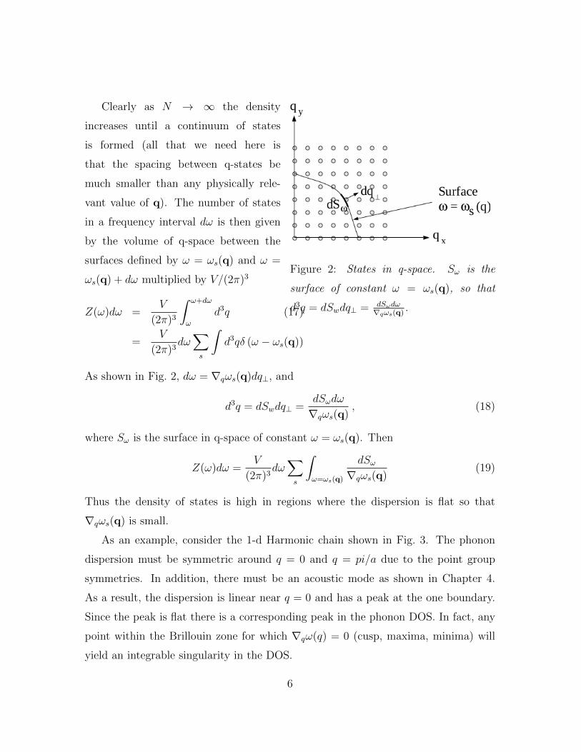
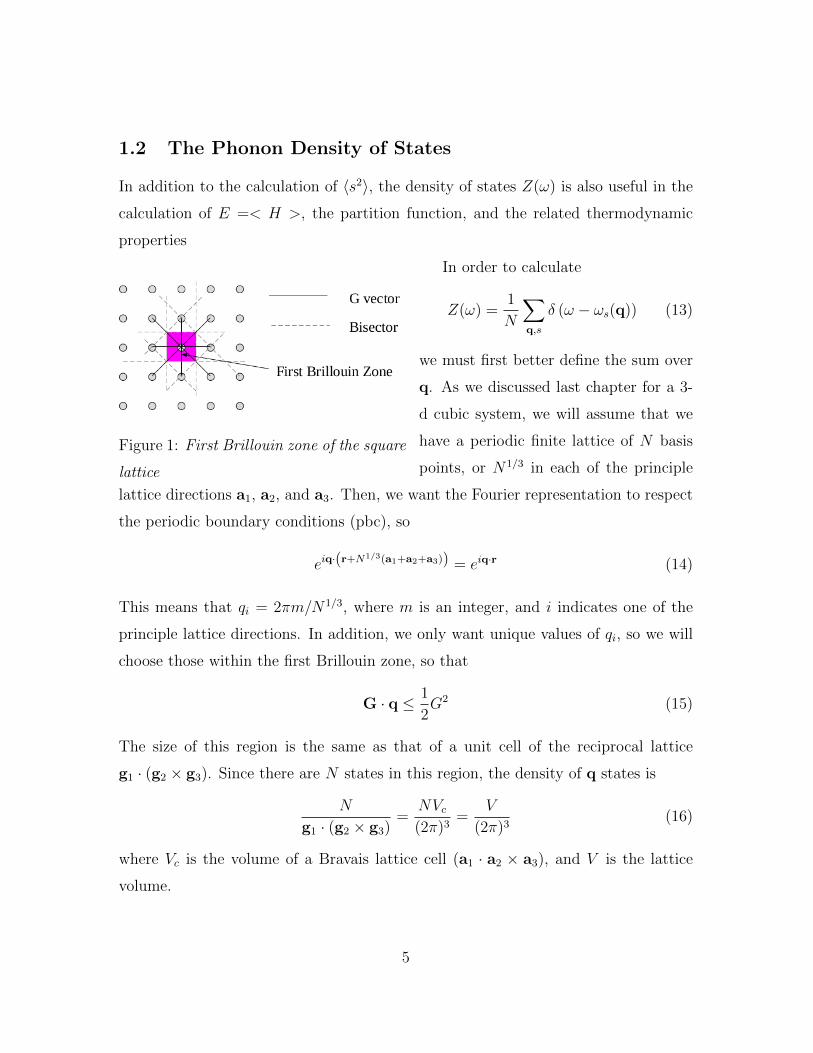
Figure 2: States in q-space. Sω is the

surface of constant ω = ωs(q), so that

d3q = dSwdq⊥ = dSωdω∇qωs(q)

.

Clearly as N → ∞ the density

increases until a continuum of states

is formed (all that we need here is

that the spacing between q-states be

much smaller than any physically rele-

vant value of q). The number of states

in a frequency interval dω is then given

by the volume of q-space between the

surfaces defined by ω = ωs(q) and ω =

ωs(q) + dω multiplied by V/(2π)3

Z(ω)dω =V

(2π)3

∫ ω+dω

ω

d3q (17)

=V

(2π)3dω∑s

∫d3qδ (ω − ωs(q))

As shown in Fig. 2, dω = ∇qωs(q)dq⊥, and

d3q = dSwdq⊥ =dSωdω

∇qωs(q), (18)

where Sω is the surface in q-space of constant ω = ωs(q). Then

Z(ω)dω =V

(2π)3dω∑s

∫ω=ωs(q)

dSω∇qωs(q)

(19)

Thus the density of states is high in regions where the dispersion is flat so that

∇qωs(q) is small.

As an example, consider the 1-d Harmonic chain shown in Fig. 3. The phonon

dispersion must be symmetric around q = 0 and q = pi/a due to the point group

symmetries. In addition, there must be an acoustic mode as shown in Chapter 4.

As a result, the dispersion is linear near q = 0 and has a peak at the one boundary.

Since the peak is flat there is a corresponding peak in the phonon DOS. In fact, any

point within the Brillouin zone for which ∇qω(q) = 0 (cusp, maxima, minima) will

yield an integrable singularity in the DOS.

6

Figure 3: Linear harmonic chain. The dispersion ω(q) is linear near q = 0, and flat

near q = ±π/a . Thus, the density of states (DOS) is flat near ω = 0 corresponding

to the acoustic mode (for which ∇qω(q) =constant), and divergent near ω = ω0

corresponding to the peak of the dispersion (where ∇qω(q) = 0)

2 Models of Lattice Dispersion

2.1 The Debye Model

For most thermodynamic properties, we are interested in the modes hω(q) ∼ kBT

which are low frequency modes in general. From a very general set of (symmetry)

constraints we have argued that all interacting lattices in which the total energy is

invariant to an overall arbitrary rigid shift in the location of the lattice must have at

least one acoustic mode, where for small ωs(q) = cs|q|. Thus, for the thermodynamic

properties of the lattice, we care predominantly about the limit ω(q) → 0. This

physics is rather accurately described by the Debye model.

In the Debye model, we will assume that all modes are acoustic (elastic), so that

7

Figure 4: Dispersion for the diatomic linear chain. In the Debye model, we replace

the acoustic mode by a purely linear mode and ignore any optical modes.

ωs(q) = cs|q| for all s and q, then ∇qωs(q) = cs for all s and q, and

Z(ω) =V

(2π)3

∑s

∫dSω∇qωs(q)

=V

(2π)3

∑s

∫dSωcs

(20)

The surface integral may be evaluated, and yields a constant∫dSω = Ss for each

branch. Typically cs is different for different modes. However, we will assume that

the system is isotropic, so cs = c. If the dispersion is isotopic, then the surface of

constant ωs(q) is just a sphere, so the surface integral is trivial

Ss(ω = ω(q)) =

2 for d = 1

2πq = 2πω/c for d = 2

4πq2 = 4πω2/c2 for d = 3

(21)

8

Figure 5: Helium on a Vycor surface. Each He is attracted weakly to the surface by a

van der Waals attraction and sits in a local minimum of the surface lattice potential.

then since the number of modes = d

Z(ω) =V

(2π)3

2/c for d = 1

2πq = 4πω/c2 for d = 2

4πq2 = 12πω2/c3 for d = 3

0 < ω < ωD (22)

Note that since the total number of states is finite, we have introduced a cutoff ωD

on the frequency.

2.2 The Einstein Model

“Real” two dimensional systems, i.e., a monolayer of gas (He) deposited on an atom-

ically perfect surface (Vycor), may be better described by an Einstein model where

each atom oscillates with a frequency ω0 and does not interact with its neighbors. The

model is dispersionless ω(q) = ω0, and the DOS for this system is a delta function

Z(ω) = cδ(ω − ω0). Note that it does not have an acoustic mode; however, this is

not in violation of the discussion in the last chapter. Why?

3 Thermodynamics of Crystal Lattices

We are now in a situation to calculate many of the thermodynamic properties of

crystal lattices. However before addressing such questions as the lattice energy free

9

energy and specific heat we should see if our model has long-range order... ie., is it

consistent with our initial assumptions.

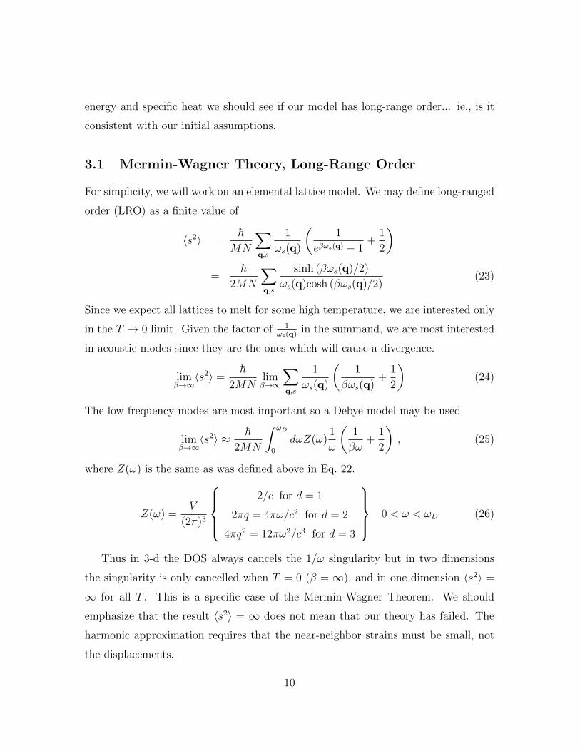
3.1 Mermin-Wagner Theory, Long-Range Order

For simplicity, we will work on an elemental lattice model. We may define long-ranged

order (LRO) as a finite value of

〈s2〉 =h

MN

∑q,s

1

ωs(q)

(1

eβωs(q) − 1+

1

2

)=

h

2MN

∑q,s

sinh (βωs(q)/2)

ωs(q)cosh (βωs(q)/2)(23)

Since we expect all lattices to melt for some high temperature, we are interested only

in the T → 0 limit. Given the factor of 1ωs(q)

in the summand, we are most interested

in acoustic modes since they are the ones which will cause a divergence.

limβ→∞〈s2〉 =

h

2MNlimβ→∞

∑q,s

1

ωs(q)

(1

βωs(q)+

1

2

)(24)

The low frequency modes are most important so a Debye model may be used

limβ→∞〈s2〉 ≈ h

2MN

∫ ωD

0

dωZ(ω)1

ω

(1

βω+

1

2

), (25)

where Z(ω) is the same as was defined above in Eq. 22.

Z(ω) =V

(2π)3

2/c for d = 1

2πq = 4πω/c2 for d = 2

4πq2 = 12πω2/c3 for d = 3

0 < ω < ωD (26)

Thus in 3-d the DOS always cancels the 1/ω singularity but in two dimensions

the singularity is only cancelled when T = 0 (β = ∞), and in one dimension 〈s2〉 =

∞ for all T . This is a specific case of the Mermin-Wagner Theorem. We should

emphasize that the result 〈s2〉 = ∞ does not mean that our theory has failed. The

harmonic approximation requires that the near-neighbor strains must be small, not

the displacements.

10

〈s2〉 d = 1 d = 2 d = 3

T = 0 ∞ finite finite

T 6= 0 ∞ ∞ finite

Table 1: 〈s2〉 for lattices of different dimension, assuming the presence of an acoustic

mode.

Figure 6: Random fluctuaions of atoms in a 1-d lattice may accumulate to produce a

very large displacements of the atoms.

Physically, it is easy to understand why one-dimensional systems do not have

long range order, since as you go along the chain, the displacements of the atoms can

accumulate to produce a very large rms displacement. In higher dimensional systems,

the displacements in any direction are constrained by the neighbors in orthogonal

directions. “Real” two dimensional systems, i.e., a monolayer of gas deposited on an

atomically perfect surface, do have long-range order even at finite temperatures due

to the surface potential (corrugation of the surface). These may be better described

by an Einstein model where each atom oscillates with a frequency ω0 and does not

interact with its neighbors. The DOS for this system is a delta function as described

11

above. For such a DOS, 〈s2〉 is always finite. You will explore this physics, in much

more detail, in your homework.

3.2 Thermodynamics

We will assume that our system is in equilibrium with a heat bath at temperature T .

This system is described by the canonical ensemble, and may be justified by dividing

an infinite system into a finite number of smaller subsystems. Each subsystem is

expected to interact weakly with the remaining system which also acts as the subsys-

tems heat bath. The probability that any state in the subsystem is occupied is given

by

P ({ns(k)}) ∝ e−βE({ns(k)}) (27)

Thus the partition function is given by

Z =∑{ns(k)}

e−βE({ns(k)})

=∑{ns(k)}

e−β∑

k,s hωs(k)(ns(k)+ 12)

=∏s,k

Zs(k) (28)

where Zs(k) is the partition function for the mode s,k; i.e. the modes are independent

and decouple.

Zs(k) =∑n

e−βhωs(k)(ns(k)+ 12)

= e−βhωs(k)/2∑n

e−βhωs(k)(ns(k))

=e−βhωs(k)/2

1− e−βhωs(k)

=1

2 sinh (βωs(k)/2)(29)

The free energy is given by

F = −kBT ln (Z) = kBT∑k,s

ln (2 sinh (βhωs(k)/2)) (30)

12

Since dE = TdS − PdV and dF = TdS − PdV − TdS − SdT , the entropy is

S = −(∂F∂T

)V

, (31)

and system energy is then given by

E = F + TS = F − T(∂F∂T

)V

(32)

where constant volume V is guaranteed by the harmonic approximation (since <

s >= 0).

E =∑k,s

1

2hωs(k)coth (βωs(k)/2) (33)

The specific heat is then given by

C =

(dEdT

)V

= kB∑k,s

(βhωs(k))2 csch2 (βωs(k)/2) (34)

where csch (x) = 1/sinh (x)

Consider the specific heat of our 3-dimensional Debye model.

C = kB

∫ ωD

0

dωZ(ω) (βω/2)2 csch2 (βω/2)

= kB

∫ ωD

0

dω

(12V πω2

(2πc)3

)(βω/2)2 csch2 (βω/2) (35)

Where the Debye frequency ωD is determined by the requirement that

3rN =

∫ ωD

0

dωZ(ω) =

∫ ωD

0

dω

(12V πω2

(2πc)3

), (36)

or V/(2πc)3 = 3rN/(4ω3D).

Clearly the integral for C is a mess, except in the high and low T limits. At high

temperatures βhωD/2� 1,

C ≈ kB

∫ ωD

0

dωZ(ω) = 3NrkB (37)

This is the well known classical result (equipartition theorem) which attributes (1/2)kB

of the specific heat to each quadratic degree of freedom. Here for each element of

13

the basis we have 6 quadratic degrees of freedom (three translational, and three mo-

menta).

At low temperatures, βhω/2� 1,

csch2 (βω/2) ≈ 2e−βω/2 (38)

Thus, at low T , only the low frequency modes contribute, so the upper bound of

integration may be extended to ∞

C ≈ 12πkB3rN

4ω2D

∫ ∞0

dωω2

(βhω

2

)2

2e−βωs(k)/2 . (39)

If we make the change of variables x = βhω/2, we get

C ≈ 9kBrNπ

2

(1

ωDβh

)3 ∫ ∞0

dxx4e−x (40)

≈ 9kBrNπ

2

(1

ωDβh

)3

24 (41)

Then, if we identify the Debye temperature θD = hωD/kB, we get

C ≈ 96πrNkB

(T

θD

)3

(42)

C ∝ T 3 at low temperature is the characteristic signature of low-energy phonon exci-

tations.

3.3 Thermal Expansion, the Gruneisen Parameter

Consider a cubic system of linear dimension L. If unconstrained, we expect that the

volume of this system will change with temperature (generally expand with increasing

T , but not always. cf. ice or Si). We define the coefficient of free expansion (P = 0)

as

αL =1

L

dL

dTor αV = 3αL =

1

V

dV

dT. (43)

Of course, this measurement only makes sense in equilibrium.

P = −(dFdV

)T

= 0 (44)

14

Figure 7: Plot of the potential V (x) = 12mx2 + cx3 when m = ω = 1 and c = 0.0, 0.1.

The average position of a particle < x > in the anharmonic potential, c = 0.1, will

shift to the left as the energy (temperature) is increased; whereas, that in the harmonic

potential, c = 0, is fixed < x >= 0.

As mentioned earlier, since < s >= 0 in the harmonic approximation, a harmonic

crystal does not expand when heated. Of course, real crystals do, so that lack of ther-

mal expansion of a harmonic crystal can be considered a limitation of the harmonic

theory. To address this limitation, we can make a quasiharmonic approximation.

Consider a more general potential between the ions, of the form

V (x) = bx+ cx3 +1

2mω2x2 (45)

and let’s see if any of these terms will produce a temperature dependent displacement.

The last term is the usual harmonic term, which we have already shown does not

produce a T-dependent < x >. Also the first term does not have the desired effect!

It corresponds to a temperature-independent shift in the oscillator, as can be seen by

completing the square

1

2mω2x2 + bx =

1

2

(x+

b

mω2

)2

− b2

2mω2. (46)

Then < x >= − bmω2 , independent of the temperature; that is, assuming that b is

temperature-independent. What we need is a temperature dependent coefficient b!

The cubic term has the desired effect. As can be seen in Fig 7, as the average

energy (temperature) of a particle trapped in a cubic potential increases, the mean

15

position of the particle shifts. However, it also destroys the solubility of the model.

To get around this, approximate the cubic term with a mean-field decomposition.

cx3 ≈ cηx⟨x2⟩

+ c(1− η)x2 〈x〉 (47)

and treat these two terms separately (the new parameter η is to be determined self-

consistently, usually by minimizing the free energy with respect to η). The first term

yields the needed temperature dependent shift of < x >

1

2mω2x2 + cηx

⟨x2⟩

=1

2mω2

(x+

cη < x2 >

mω2

)2

− c2 < x2 >2

2mω2(48)

so that < x >= − cη<x2>mω2 . Clearly the renormalization of the equilibrium position

of the harmonic oscillator will be temperature dependent. While the second term,

(1− η)x2 < x >, yields a shift in the frequency ω → ω′

ω′ = ω

(1 +

2(1− η) < x >

mω2

) 12

(49)

which is a function of the equilibrium position. Thus a mean-field description of the

cubic term is consistent with the observed physics.

In what follows, we will approximate the effect of the anharmonic cubic term as

a shift in the equilibrium position of the lattice (and hence the lattice potential) and

a change of ω to ω′; however, we imagine that the energy levels remain of the form

En = hω′(< x >)(n+1

2), (50)

and that < x > varies with temperature, consistent with the mean-field approxima-

tion just described.

To proceed, imagine the cube of cubic system to be made up of oscillators which are

independent. Since the final result can be formulated as a sum over these independent

modes, consider only one. In equilibrium, where P = −(dFdV

)T

= 0, the free energy

of one of the modes is

F = Φ +1

2hω + kBT ln

(1− e−βhω

)(51)

16

and (following the notation of Ibach and Luth), let the lattice potential

Φ = Φ0 +1

2f(a− a0)2 + · · · (52)

where f is the spring constant. Then

0 = P =

(dFda

)T

= f(a− a0) +1

ω

∂ω

∂a

(1

2hω − hω

1− e−βhω

), (53)

If we identify the last term in parenthesis as ε(ω, T ), and solve for a, then

a = a0 −1

ωfε(ω, T )

∂ω

∂a(54)

Since we now know a(T ) for a single mode, we may calculate the linear expansion

coefficient for this mode

αL =1

a0

da

dT= − 1

a20f

∂ lnw

∂ ln a

∂ε(ω, T )

∂T(55)

To generalize this to a solid let αL → αV (as discussed above) and a20f → V 2 dP

dV= V κ

(κ is the bulk modulus) and sum over all modes the modes k, s

αV =1

V

dV

dT=

1

κV

∑k,s

−∂ lnωs(k)

∂ lnV

∂ε (ωs(k), T )

∂T. (56)

Clearly (due to the factor of ∂ε∂T

), αV will have a behavior similar to that of the

specific heat (αV ∼ T 3 for low T , and αV =constant for high T ). In addition, for

many lattices, the Gruneisen number

γ =∂ lnωs(k)

∂ lnV(57)

shows a weak dependence upon s,k, and may be replaced by its average, called the

Gruneisen parameter

〈γ〉 =

⟨∂ lnωs(k)

∂ lnV

⟩, (58)

typically on the order of two.

17

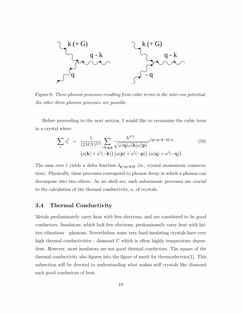
Figure 8: Three-phonon processes resulting from cubic terms in the inter-ion potential.

Six other three-phonon processes are possible.

Before proceeding to the next section, I would like to reexamine the cubic term

in a crystal where∑l

s3l =

1

(2MN)3/2

∑l,k,q,p

h3/2√ω(q)ω(k)ω(p)

ei(p+q+k−G)·rl (59)(a(k) + a†(−k)

) (a(p) + a†(−p)

) (a(q) + a†(−q)

).

The sum over l yields a delta function δp+q+k,G (ie., crystal momentum conserva-

tion). Physically, these processes correspond to phonon decay in which a phonon can

decompose into two others. As we shall see, such anharmonic processes are crucial

to the calculation of the thermal conductivity, κ, of crystals.

3.4 Thermal Conductivity

Metals predominately carry heat with free electrons, and are considered to be good

conductors. Insulators, which lack free electrons, predominantly carry heat with lat-

tice vibrations – phonons. Nevertheless, some very hard insulating crystals have very

high thermal conductivities - diamond C which is often highly temperature depen-

dent. However, most insulators are not good thermal conductors. The square of the

thermal conductivity also figures into the figure of merit for thermoelectrics[1]. This

subsection will be devoted to understanding what makes stiff crystals like diamond

such good conductors of heat.

18

material/T 273.2K 298.2K

C 26.2 23.2

Cu 4.03 4.01

Table 2: The thermal conductivities of copper and diamond (CRC) ( in µOhm-cm).

The thermal conductivity κ is measured by setting up a small steady thermal

gradient across the material, then

Q = −κ∇T (60)

where Q is the thermal current density; i.e., the energy times the density times the

velocity. If the thermal current is in the x-direction, then

Qx =1

V

∑q,s

hωs(q)〈ns(q)〉vsx(q) (61)

where the group velocity is given by vsx(q) = ∂ωs(q)∂qx

. Since we assume ∇T is small,

we will only look at the linear response of the system where 〈ns(q)〉 deviates little

from its equilibrium value 〈ns(q)〉0. Furthermore since ωs(q) = ωs(−q),

vsx(−q) =∂ωs(−q)

∂ − qx= −vsx(q) (62)

Thus as 〈ns(−q)〉0 = 〈ns(q)〉0

Q0x =

1

V

∑q,s

hωs(q)〈ns(q)〉0vsx(q) = 0 (63)

since the sum is over all q in the B.Z. Thus if we expand

〈ns(q)〉 = 〈ns(q)〉0 + 〈ns(q)〉1 + · · · (64)

we get

Qx ≈1

V

∑q,s

hωs(q)〈ns(q)〉1vsx(q) (65)

19

Figure 9: Change of phonon density within a trapazoidal region. 〈ns(q)〉 can change

either by phonon decay or by phonon diffusion into and out of the region.

since we presumably already know ωs(k), the calculation of Q and hence κ reduces

to the evaluation of the linear change in < n >.

Within a region, < n > can change in two ways. Either phonons can diffuse into

the region, or they can decay through an anharmonic (cubic) term into other modes.

sod〈n〉dt

=∂〈n〉∂t

∣∣∣∣diffusion

+∂〈n〉∂t

∣∣∣∣decay

(66)

However d〈n〉dt

= 0 since we are in a steady state. The decay process is usually described

by a relaxation time τ (or a mean-free path l = vτ )

∂〈n〉∂t

∣∣∣∣decay

= −< n > − < n >0

τ=≈ −< n >1

τ(67)

The diffusion part of d〈n〉dt

is addressed pictorially in Fig. 10. Formally,

∂〈n〉∂t

∣∣∣∣diffusion

≈ 〈n(x− vx∆t)〉 − 〈n(x)〉∆t

≈ −∂〈n(x)〉∂x

vx (68)

≈ −vx∂〈n(x)〉∂T

∂T

∂x≈ −vx

∂ (〈n(x)〉0 + 〈n(x)〉1)

∂T

∂T

∂x

Keeping only the lowest order term,

∂〈n〉∂t

∣∣∣∣diffusion

≈ −vx∂〈n(x)〉0

∂T

∂T

∂x(69)

20

Figure 10: Phonon diffusion. In time ∆t, all the phonons in the left, source region,

will travel into the region of interest on the right, while those on the right region will

all travel out in time ∆t. Thus, ∆n/∆t = (nleft − nright)/∆t.

Then as d〈n〉dt

= 0,∂〈n〉∂t

∣∣∣∣diffusion

= − ∂〈n〉∂t

∣∣∣∣decay

(70)

or

〈n〉1 = −vxτs(q)∂〈n(x)〉0

∂T

∂T

∂x. (71)

Thus

Qx ≈ −1

V

∑q,s

hωs(q)v2sx(q)τs(q)

∂〈n(x)〉0

∂T

∂T

∂x, (72)

and since Q = −κ∇T

κ ≈ 1

V

∑q,s

hωs(q)v2sx(q)τ

∂〈n(x)〉0

∂T. (73)

From this relationship we can learn several things. First since κ ∼ v2sx(q), phonons

near the zone boundary or optical modes with small vs(q) = ∇qωs(q) contribute little

to the thermal conductivity. Also, stiff materials, with very fast speed of the acoustic

modes vsx(q) ≈ c will have a large κ. Second, since κ ∼ τs(q), and ls(q) = vsx(q)τs(q),

κ will be small for materials with short mean-free paths. The mean-free path is

effected by defects, anharmonic Umklapp processes, etc. We will explore this effect,

especially its temperature dependence, in more detail.

21

Figure 11: Umklapp processes involve a reciprocal lattice vector G in lattice momen-

tum conservation. They are possible whenever q1 > G/2, for some G, and involve a

virtual reversal of the momentum and heat carried by the phonons (far right).

At low T , only low-energy, acoustic, modes can be excited (those with hωs(q) ∼kBT ). These modes have

vs(q) = cs (74)

In addition, since the momentum of these modes q � G, we only have to worry about

anharmonic processes which do not involve a reciprocal lattice vector G in lattice

momentum conservation. Consider one of the three-phonon anharmonic processes

of phonon decay shown in Fig. 8 (with G = 0). For these processes Q ∼ hωc so

the thermal current is not disturbed by anharmonic processes. Thus the anharmonic

terms at low T do not affect the mean-free path, so the thermal resistivity (the inverse

of the conductivity) is dominated by scattering from impurities in the bulk and surface

imperfections at low temperatures.

At high T momentum conservation in an anharmonic process may involve a re-

ciprocal lattice vector G if the q1 of an excited mode is large enough and there exists

a sufficiently small G so that q1 > G/2 (c.f. Fig. 11). This is called an Umklapp

process, and it involves a very large change in the heat current (almost a reversal).

Thus the mean-free path l and κ are very much smaller for high temperatures where

q1 can be larger than half the smallest G.

So what about diamond? It is very hard and very stiff, so the sound velocities cs

22

are large, and so thermally excited modes for which kBT ∼ hω ∼ hcq involve small

q1 for which Umklapp processes are irrelevant. Second κ ∼ c2 which is large. Thus κ

for diamond is huge!

References

[1] https://en.wikipedia.org/wiki/Thermoelectric materials

23