Chapter 5 – Sections 5.5 – 5.9

H.Imesh Neeran Gunaratna

PSU ID: 901129894

Portland State UniversityMicrowave Circuit Design – ECE 531

By David M.Pozar

Index:

• Introduction: The Quarter-Wave Transformer………………………… slide 3

• Section 5.5 – The Theory of Small Reflections…………………………. slide 7

• Section 5.6 – Binomial Multisection Matching Transformers…… slide 17

• Section 5.7 – Chebyshev Multisection Matching Transformers… slide 24

• Section 5.8 – Tapered Lines………………………………………………….. slide 28

• Section 5.9 – The Bode- Fano Criterion………………………………….. slide 31

Introduction: Quarter-Wave Transformer

• Definition: The quarter-wave transformer is a useful and

practical circuit for impedance matching and also provides a simple transmission line circuit that further illustrates the properties of standing waves on a mismatched line.

Let me explain with an example.

• Say the end of a transmission line with characteristic impedance Z0 is terminated with a resistive (i.e., real) load.

• We typically would like all power traveling down the line to be

absorbed by the load RL.

• But if RL ≠Z0 , the line is unmatched and some of the incident power will be reflected.

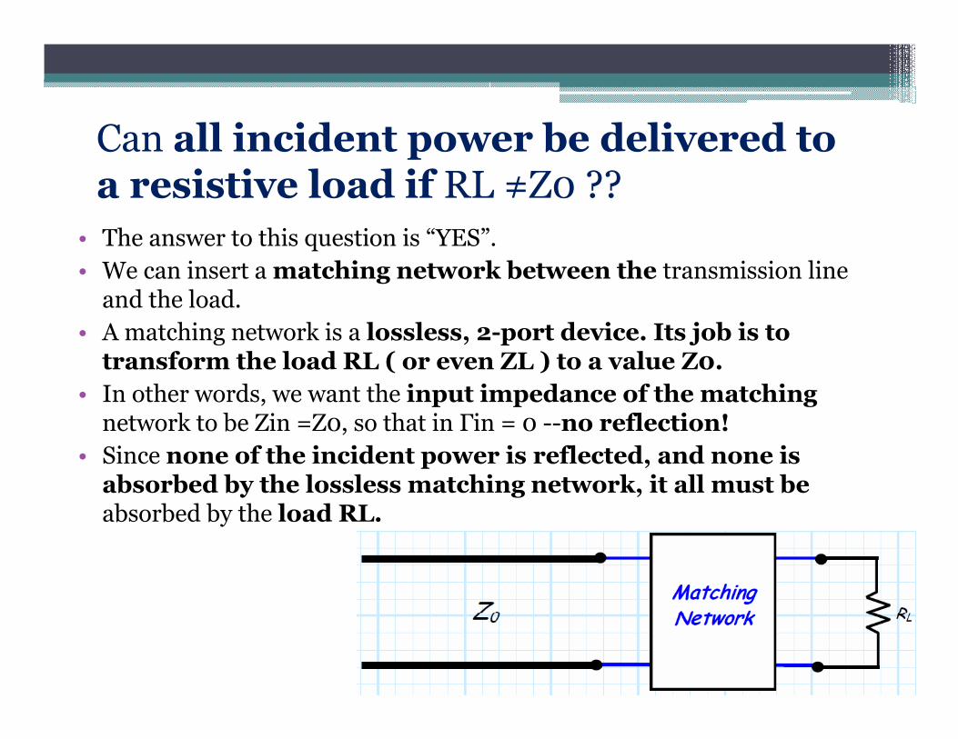
Can all incident power be delivered to a resistive load if RL ≠Z0 ??

• The answer to this question is “YES”.

• We can insert a matching network between the transmission line and the load.

• A matching network is a lossless, 2-port device. Its job is to transform the load RL ( or even ZL ) to a value Z0.

• In other words, we want the input impedance of the matching network to be Zin =Z0, so that in Γin = 0 --no reflection!

• Since none of the incident power is reflected, and none is absorbed by the lossless matching network, it all must be absorbed by the load RL.

How can we build a matching network?

• The easiest is the quarter-wave transformer

• First, insert a transmission line with characteristic impedance

• Z1 and length l = λ/4 (i.e., a quarter-wave line) between the load and the Z0 transmission line.

The λ 4 line is the matching network

• The quarter wavelength case is one of the special cases that we studied. We know that the input impedance of the quarter wavelength line is:

• Thus, if we wish for Zin to be numerically equal to Z0, we find:

• Solving for Z1, we find its required value to be:

• Thus, all power is delivered to load RL

• Important Note: We find that in Z0 =Zin only if the matching quarter-wave transmission line is exactly one-quarter wavelength in length

l = λ/4.

• The problem with this, of course, is that a physical length l of transmission line is exactly one-quarter wavelength at only one frequency f.

• Remember, wavelength is related to frequency as:

• One drawback of the quarter-wave transformer is that it can only match a real load impedance. A complex load impedance can always be transformed to a real impedance by using an appropriate length of transmission line between the load and the transformer, or an appropriate series or shunt reactive stub.

• Another drawback of the quarter-wave transformer is that a quarter-wave transformer provides a perfect match ( Γ = 0 ) at only one signal frequency

Section 5.5-The Theory of Small Reflections

• The quarter-wave transformer provides simple means of matching any real load impedance to any line impedance. For applications requiring more bandwidth than a single quarter-wave section can provide, multisection transformers can be used.

• When designing these transformers, total reflection coefficient caused by the partial reflections from small discontinuities in the transmission line have to be considered.

What are discontinuities?

By either necessity or design, microwave networks often consist of transmission lines with various types of transmission line discontinuities. Discontinuities may be unavoidable result of mechanical or electrical transitions from one medium to another. For instance like a junction between a two waveguides.

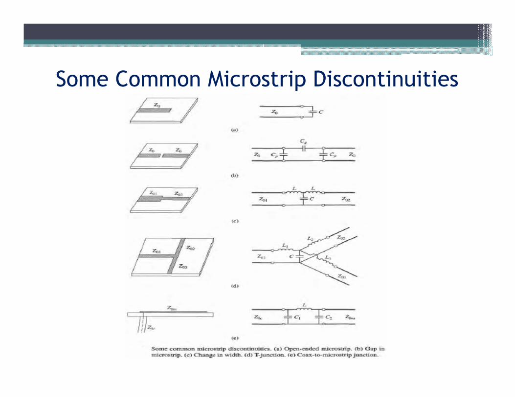
Some Common Microstrip Discontinuities

Single Section Transformer

• Consider the single-section transformer shown below.

• We will derive an approximate expression for the overall reflection coefficient Γ.

-T12T21 Γ3

T12T21 Γ3 Γ3 Γ2

Γ1

This expression can be further simplified using the geometric series

Multisection Transformer• Consider a sequence of N transmission line sections; each section has

equal length “l”, but dissimilar characteristic impedances:

• The partial reflection coefficients can be defined at each junction, as follows,

• Note that since RL is real, and since we assume lossless transmission lines, all Γn will be real.

• If the load resistance RL is less than Z0 , then we should design the transformer such that:

Z 0>Z1 >Z2 >Z3……> ZN >RL

• Conversely, if RL is greater than Z0 , then we will design the transformer such that:

Z 0 <Z1 <Z2 <Z3…..<ZN <RLIn other words, we gradually transition from Z0 to RL.

• Hence, this proves the fact that Zn increase or decrease monotonically across the transformer, and that ZL is real.

• Here, we can apply the “theory of small reflections”to analyze this multi-section transformer.

• The theory of small reflections allows us to approximate the input reflection coefficient of the transformer as follows,

•

• Signal Flow Diagram (read section 4.5)

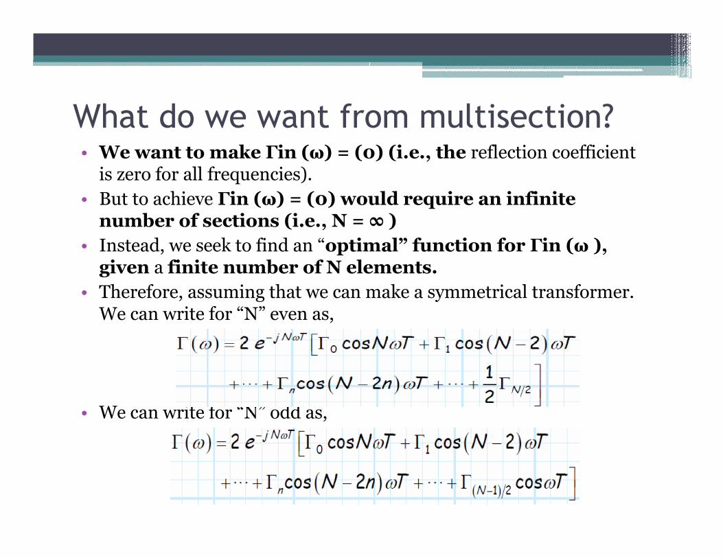
What do we want from multisection?• We want to make Γin (ω) = (0) (i.e., the reflection coefficient

is zero for all frequencies).

• But to achieve Γin (ω) = (0) would require an infinite number of sections (i.e., N = ∞ )

• Instead, we seek to find an “optimal” function for Γin (ω ), given a finite number of N elements.

• Therefore, assuming that we can make a symmetrical transformer. We can write for “N” even as,

• We can write for “N” odd as,

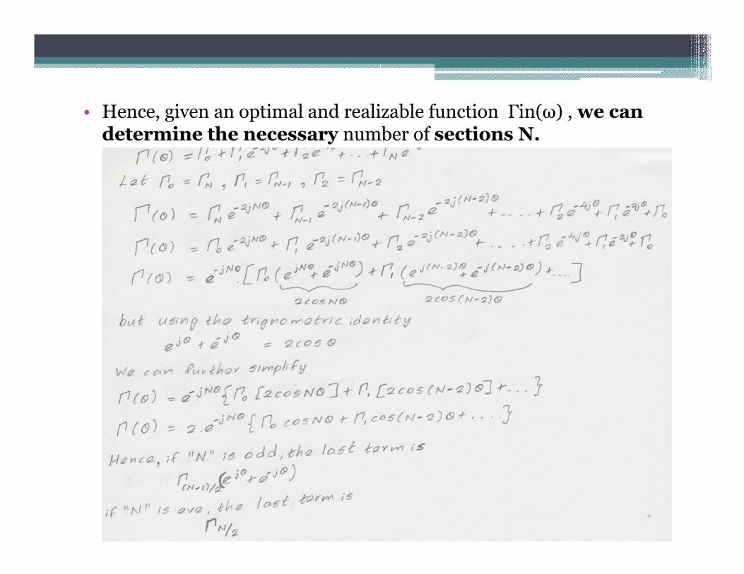
• Hence, given an optimal and realizable function Γin(ω) , we can determine the necessary number of sections N.

Section 5.6 – Binomial Multisection

Matching Transformers• The pass band response of a binomial matching transformer is

optimum in the sense that for a given number of sections. It can be known as maximally flat. This type of response is designed for an N-section transformer, by setting the first N-1 derivatives of l Γ(θ) to zero, at the center frequency f0.

• We need to define N independent design equations, which we can then use to solve for the N values of characteristic impedance Zn .

• First, we start with a single design frequency ω0 , where we wish to achieve a perfect match:

Γin (ω = ω0 ) = 0

• That’s just one design equation: we need N-1 more.

• One such criterion is to make the function Γin(ω) maximally flat at the point ω0 = ω .

• We found that this function has a matching network of Γ(θ ) = 0 at θ = π/2--a perfect match

• Additionally, the function is maximally flat at θ = π/2, therefore Γ(θ ) ≈ 0 over a wide range around θ = π/2--a wide bandwidth.

• But how does θ = π/2 relate to frequency ω????

• θ = βl

• Where β = 2π/λ and λ = V/ω

• This (ω0 ) is our design frequency—the frequency where we have a perfect match.

• Note that the length “l” has an interesting relationship with this frequency:

• When l = λ/4

• Binomial Multi-section matching network will have a perfect match at the frequency where the section lengths “l”are a quarter wavelength.

• First design rule: Set section lengths “l” so that they are a quarter wave length ( λ0/4) at the design frequency ω0 .

• What is the value of A ??

• We can determine this value by evaluating a boundary condition.

• We can easily determine the value of Γ(ω ) at ω = 0.

• Note as ω approaches zero, the electrical length βl of each section will likewise approach zero. Thus, the input impedance Zin will simply be equal to RL as ω→ 0.

• As a result, the input reflection coefficient Γ(ω = 0) must be:

• And we found out that,

• By equating the two expressions we get,

• Hence

• Now have a form for the partial reflection coefficients Γn :

• But we also know that the partial reflection coefficients Γn is also,

• We know that the values of n 1 Z + and n Z are typically very close, such that Zn+1 - Zn is small.

• Note that as we increase the number of sections, the matching bandwidth increases.

• As we move from the design (perfect match) frequency f0 the value Γ(f ) will increase. At some frequency (fm, say) the magnitude of the reflection coefficient will increase to some unacceptably high value ( Γm , say). At that point, we no longer consider the device to be matched.

• Note there are two values of frequency fm —one value less than design frequency f0, and one value greater than design frequency f0. These two values define the bandwidth of the matching network.

let Γm be the maximum value of reflection coefficient that can be tolerated over the passband

Fractional bandwidth

Section 5.7 – Chebyshev Multisection

Matching Transformers• We can also build a multisection matching network such that the

function Γ(f ) is a Chebyshev function.

• Chebyshev functions maximize bandwidth, although at the cost of pass-band ripple.

• Chebyshev solutions can provide functions Γ(ω ) with wider

• bandwidth than the Binomial case—although at the “expense” of passband ripple.

• Chebyshev transformers are symmetric.

• The reflection coefficient of a Chebyshev matching network has the form: where θm =ωmT

• The function TN(cos θ sec θ) is a Chebyshev polynomial of order N.

• The first four Chebyshev polynomials are,

• Inserting the substitution: x = cosθsecθm into the Chebyshev polynomials above

• We can now synthesize a Chebyshev equal-ripple passband by making Γ(θ) proportional to TN(secθmcosθ) where N is the number of sections in the transformer.

• As in the binomial transformer case we can find the constant “A” by letting θ = 0 at zero frequency.

• The maximum allowable reflection coefficient magnitude in the passband is Γm.

• But Γm = lAl

• The maximum value of TN(secθmcosθ) is in the passband is unity.

• We can find θm by using,

• The fractional bandwidth can be calculated using the following equation once θm is known.

• Summarizing the he Chebyshev matching network design procedure

• 1. Determine the value N required to meet the bandwidth and

ripple m Γ requirements.

• 2. Determine the Chebychev function.

• 3. Determine all Γn by equating terms with the symmetric

multisection transformer expression:

• 4. Calculate all Zn using the approximation:

• 5. Determine section length l = λ0/4.

Section 5.8 – Tapered Lines• What is taper? It’s the gradual diminution of thickness, diameter, or

width in an elongated object.

• In this section the matching is done by discrete sections, while line is continuously tapered.

The total reflection coefficient at z = 0 can be found by summing all the partial reflections with their appropriate phase shifts.

Exponential, Triangular &Klopfenstein Taper

Consider first an exponential taper, whereZ(z) = Z0eqz for 0 < z < L ,

At z = 0, Z (0) = Z0

At z = L, we want to have Z (L) = ZL = Z0eaL

Constant “a” is derived as,

•We can find Γ(θ) by using the previous equation.•The magnitude of the reflection coefficient decreases as length increases as shown above.

Reflection coefficient magnitude vs frequency for tapers

Section 5.9 – The Bode-Fano Criterion

• When a lossless network is used to match an arbitrary complex load, generally over a nonzero bandwidth. Some questions may arise.

• Can we achieve a perfect match (zero reflection) over a specified bandwidth?

• If not, how well can we do? What is the trade-off between Γm, the maximum allowable reflection in the passband, and the bandwidth?

• How complex must the matching network be for a given specification?

• These questions can be answered by the Bode-Fano criterion.

• Bode-Fano Criterion gives certain canonical types of load impedances, a theoretical limit on the minimum reflection coefficient magnitude that can be obtained with an arbitrary matching network. Thus represents the optimum result that can be ideally achieved, even though such a result may only be approximated in practice.

Bode-Fano Limits for RC and RL loads

matched with networks