Chapter 5. Regression Modelsthaddeus.tarpey/STT363chapter5.pdfChapter 5: Regression Models 118 April 9, 2013 ... we ﬁrst return to the very simple model introduced in Chapter 1 to

Chapter 5: Regression Models 118

April 9, 2013

Chapter 5. Regression Models

Regression analysis is probably the most used tool in statistics. Regression deals withmodeling how one variable (called a response) is related to one or more other variables(called predictors or regressors). Before introducing regression models involving twoor more variables, we first return to the very simple model introduced in Chapter 1to set up the basic ideas and notation.

1 A Simple Model

Consider once again the fill-weights in the cup-a-soup example. For sake of illustra-tion, consider the first 10 observations from the data set:

236.93, 237.39, 239.67, 236.39, 239.67, 237.26, 239.27, 237.46, 239.08, 237.83.

Note that although the filling machine is set to fill each cup to a specified weight, theactual weights vary from cup to cup. Let y1, y2, . . . , yn denote the fill-weights for oursample (i.e. y1 = 236.93, y2 = 237.39 etc. and n = 10). The model we introduced inChapter 1 that incorporates the variability is

yi = µ+ ϵi (1)

where ϵi is a random error representing the deviation of the ith diameter from theaverage fill-weight of all cups (µ). Equation (1) is a very simple example of a statisticalmodel. It involves a random component (ϵi) and a deterministic component (µ). Thepopulation mean µ is a parameter of the model and the other parameter in (1) is thevariance of the random error ϵ which we shall denote by σ2 (“sigma-squared”).

Let us now consider the problem of estimating the population mean µ in (1). Thetechnique we will use for (1) is called least-squares and it is easy to generalize to morecomplicated regression models. A natural and intuitive way of estimating the truevalue of the population mean µ is to simply take the average of the measurements:

y =1

n

n∑i=1

yi.

Why should we use y to estimate µ? There are many reasons why y is a good estimatorof µ, but the reason we shall focus on is that y is the best estimator of µ in terms ofhaving the smallest mean squared error. That is, given the 10 measurements above,we can ask: which value of µ makes sum of squared deviations

n∑i=1

(yi − µ)2 (2)


the smallest? That is, what is the least-squares estimator of µ? The answer to thisquestion can be found by doing some simple calculus. Consider the following functionof µ:

f(µ) =n∑

i=1

(yi − µ)2.

From calculus, we know that to find the extrema of a function, we can take thederivative of the function, set it equal to zero, and solve for the argument of thefunction. Thus,

d

dµf(µ) = −2

n∑i=1

(yi − µ) = 0.

Using a little algebra, we can solve this equation for µ to get

µ = y.

(One can check that the 2nd derivative of this function is positive so that setting thefirst derivative to zero determines a value of µ that minimizes the sum of squares.)

The hat notation (i.e. µ) is used to denote an estimator of a parameter. This isa standard notational practice in statistics. Thus, we use µ = y to estimate theunknown population mean µ. Note that µ is not the true value of µ but simply anestimator based on 10 data points.

Now we shall re-do the computation using matrix notation. This will seem unnec-essarily complicated, but once we have a solution worked out, we can re-apply it tomany other much more complicated models very easily. Data usually comes to us inthe form of arrays of numbers, typically in computer files. Therefore, a natural andeasy way to handle data (particularly large sets of data) is to use the power of matrixcomputations. Take the fill-weight measurements y1, y2, . . . , yn and stack them intoa vector and denote this vector by a boldfaced y:

y =

y1y2y3y4y5y6y7y8y9y10

=

236.93237.39239.67236.39239.67237.26239.27237.46239.08237.83

.

Now let X denote a column vector of ones and ϵ denote the error terms ϵis stackedinto a vector:

X =

11...1

and ϵ =

ϵ1ϵ2...ϵn

.


Then we can re-write our very simply model (1) in matrix/vector form as:y1y2...yn

=

11...1

µ+

ϵ1ϵ2...ϵn

.

More compactly, we can write:y = Xµ+ ϵ. (3)

The sum of squares in equation (2) can be written

(y −Xµ)′(y −Xµ)

Multiplying this out, we find the sum of squares to be

y′y − 2X ′yµ+ µ2X ′X.

Taking the derivative of this with respect to µ and setting the derivative equal to zerogives

−2X ′y + 2µX ′X = 0.

Solving for µ givesµ = (X ′X)−1X ′y. (4)

The solution given by equation (4) is the least squares solution and this formulaholds for a wide variety of models as we shall see.

2 The Simple Linear Regression Model

Now we will define a slightly more complicated statistical model that turns out tobe extremely useful in practice. The model is a simple extension of our first modelyi = µ + ϵi and, using the matrix notation, all we have to do is add another columnto the vector X and change it into a matrix with two columns.

To illustrate ideas, consider the data in the following table that was collected inConsumer Reports and reported on in Henderson and Velleman (1981). The tablegives the make (column 1), the miles per gallon (MPG) (Column 2) and the weight(column 3) in thousands of pounds of n = 6 Japanese cars from 1978-79 modelautomobiles.

Make MPG WeightToyota Corona 27.5 2.560Datsun 510 27.2 2.300Mazda GLC 34.1 1.975Dodge Colt 35.1 1.915Datsun 210 31.8 2.020Datsun 810 22.0 2.815


Figure 1: Scatterplot of miles per gallon versus weight of n = 6 Japanese cars.

It seems reasonable that the miles per gallon of a car is related to the weight of thecar. Our goal is to model the relationship between these two variables. A scatterplotof the data is shown in Figure 1.

As can be seen from the figure, there appears to be a linear relationship between theMPG (y) and the weight of the car (x). Heavier cars tend to have lower gas mileage.A deterministic model for this data is given by

yi = β0 + β1xi

where yi is MPG for the ith car and xi is the corresponding weight of the car. Thetwo parameters are β0 which is the y-intercept and β1 which is the slope of the line.However, this model is inadequate because it forces all the points to lie exactly ona line. From Figure 1, we clearly see that the points do follow a linear pattern,but the points do not all fall exactly on a line. Thus, a better model will includea random component for the error which allows for points to scatter about the line.The following model is called a simple linear regression model:

yi = β0 + β1xi + ϵi (5)

for i = 1, 2, . . . , n. The random variable yi is called the response (it is sometimescalled the dependent variable also). The xi is called the ith value of the regressorvariable (sometimes known as the independent or predictor variable). The randomerror ϵi is assumed to have a mean of 0 and variance σ2. We typically assume the ϵi’sare independent of each other.

The slope β1 and intercept β0 are the two parameters of primary importance andthe question arises as to how they should be estimated. The least squares solution


Figure 2: The least-squares regression line is determined by minimizing the sum ofsquared vertical differences between the observed MPG’s and the corresponding pointon the line.

is found by determining the values of β0 and β1 that minimize the sum of squarederrors:

n∑i=1

(yi − β0 − β1xi)2.

Graphically, this corresponds to finding the line minimizing the sum of squared verti-cal differences between the observed MPG’s and the corresponding values on the lineas shown in Figure 2.

Returning to our matrix and vector notation, we can write

y =

27.527.234.135.131.822.0

and X =

1 2.5601 2.3001 1.9751 1.9151 2.0201 2.815

.

Let β = (β0, β1)′ and ϵ = (ϵ1, ϵ2, . . . , ϵn)

′. Then we can rewrite (5) in matrix form as

y = Xβ + ϵ. (6)

In order to find the least-squares estimators of β, we need to find the values of β0

and β1 that minimize

(y −Xβ)′(y −Xβ) =n∑

i=1

(yi − β0 − β1xi)2


or, since ϵi = yi − β0 − β1xi, we need to find β0 and β1 that minimize ϵ′ϵ. Matrixdifferentiation can be used to solve this problem, but instead we will use a geometricargument.

First, some additional notation. Let β0 and β1 denote the least squares estimators ofβ0 and β1. Then given a value of the predictor xi, we can compute the predictedvalue of y given xi as

yi = β0 + β1xi.

The residual ri is defined to be the difference between the response yi and thepredicted value yi:

ri = yi − yi.

Let r = (r1, r2, . . . , rn)′ and y = (y1, y2, . . . , yn)

′. Note that y = Xβ where β =(β0, β1)

′. The least square estimators β0 and β1 are chosen to make r′r small as pos-sible. Geometrically, y is the projection of y onto the plane spanned by the columnsof the matrix X. This is illustrated in Figure 3. To make r′r small as possible, rshould be orthogonal to the plane spanned by the columns of X. Algebraically, thismeans that

X ′r = 0.

Writing this out, we get

X ′r = X ′(y − y)

= X ′(y −Xβ)

= 0.

Thus, β should satisfyX ′y = X ′Xβ. (7)

This equation is know as the normal equation. Assuming X ′X is an invertiblematrix, we can simply multiply on the left on both sides of (7) to get the least-squaressolution:

β = (X ′X)−1X ′y. (8)

This is one of the most important equations of this course. This formula provides theleast-squares solution for a wide variety of models. Note that we have already seenthis solution in (4).

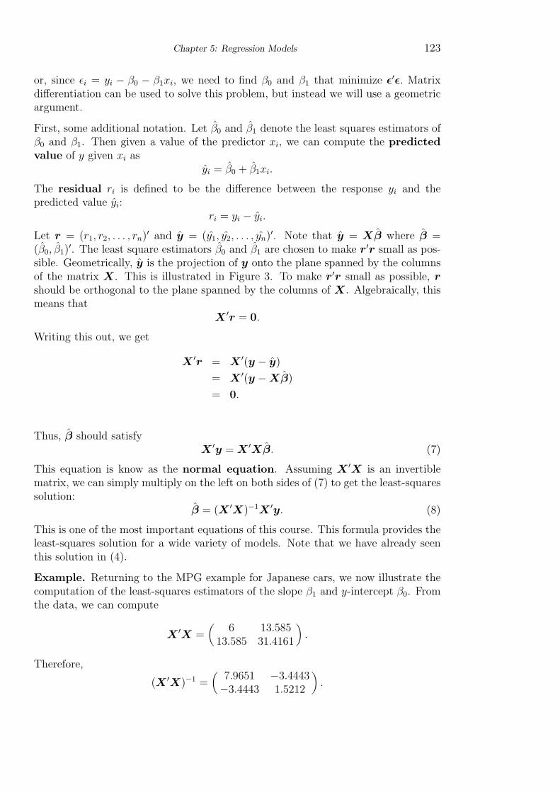
Example. Returning to the MPG example for Japanese cars, we now illustrate thecomputation of the least-squares estimators of the slope β1 and y-intercept β0. Fromthe data, we can compute

X ′X =(

6 13.58513.585 31.4161

).

Therefore,

(X ′X)−1 =(

7.9651 −3.4443−3.4443 1.5212

).


Figure 3: The geometry of least-squares. The vector y is projected onto the spacespanned by the columns of the design matrix X denoted by X1 and X2 in the figure.The projected value is the vector of fitted values y (denoted by “yhat” in the figure).The difference between y and y is the vector of residuals r.

Also,

X ′y =(

1 1 1 1 1 12.560 2.300 1.975 1.915 2.020 2.815

)

27.527.234.135.131.822.0

=

(177.70393.69

).

So, the least squares estimators of the intercept and slope are:

β = (X ′X)−1X ′y =(

7.9651 −3.4443−3.4443 1.5212

)(177.70393.69

)=

(59.4180−13.1622

).

From this computation, we find that the least squares estimator of the y-intercept isβ0 = 59.4180 and the estimated slope is β1 = −13.1622 and the prediction equationis given by

y = 59.418− 13.1622x.

Note that the estimated y-intercept of β0 = 59.418 does not have any meaningfulinterpretation in this example. The y-intercept corresponds to the average y valuewhen x = 0, i.e. the MPG for a car that weighs zero pounds. It makes no sense toestimate the mileage of a car with a weight of zero. Typically in regression examplesthe intercept will not be meaningful unless data is collected for values of x nearzero. Since there is no such thing as cars weighing zero pounds, the intercept has nomeaningful interpretation in this example.


The slope β1 is generally the parameter of primary interest in a simple linear regres-sion. The slope represents the average change in the response for a unit change inthe regressor. In the car example, the estimated slope of β1 = −13.1622 indicatesthat for each additional thousand pounds of weight of a car we would expect to seea reduction of about 13 miles per gallon on average.

Multiplying out the matrices in (8) we get the following formulas for the least squareestimates in simple linear regression:

β0 = y − β1x

β1 =SSxy

SSxx

where

SSxy =n∑

i=1

(xi − x)(yi − y)

and

SSxx =n∑

i=1

(xi − x)2.

That is, the estimator of the slope is the covariance between the x’s and y’s divided bythe variance of the x’s. In multiple regression when there is more than one regressorvariable, the formulas for the least square estimators become extremely complicatedunless you stick with the matrix notation.

The matrix notation also allows us to compute quite easily the standard errors of theleast squares estimators as well as the covariance between the estimators. First, letus show that the least square estimators are unbiased for the corresponding modelparameters. Before doing so, note that in a designed experiment, the values of theregressor are typically fixed by the experimenter and therefore are not consideredrandom. On the other hand, because yi = β0 + β1xi + ϵi and ϵi is a random variable,then yi is also a random variable. Computing, we get

E[β] = E[(X ′X)−1X ′y]

= (X ′X)−1X ′E[y]

= (X ′X)−1X ′E[Xβ + ϵ]

= (X ′X)−1X ′(Xβ + E[ϵ])

= (X ′X)−1X ′Xβ + 0

= β

since E[ϵ] = 0. Therefore, the least square estimators β are unbiased for the popula-tion parameters β.

Many statistical software packages have built-in functions that will perform regressionanalysis. We can also use software to do the matrix calculations directly. Below isMatlab code that produces some of the output generated above for the car mileageexample:


% Motor Trend car data

% Illustration of simple linear regression.

mpg = [27.5; 27.2; 34.1; 35.1; 31.8; 22.0]; % Car’s weight

wt = [2.560; 2.300; 1.975; 1.915; 2.020; 2.815];

% Compute means and standard deviations:

mean(wt)

std(wt)

mean(mpg)

std(mpg)

n = length(mpg); % n = sample size

X = [ones(6,1) wt]; % Compute the design matrix X

bhat = inv(X’*X)*X’*mpg; % bhat = estimated regression coefficients

yhat = X*bhat; % yhat = fitted values

r = mpg - yhat; % r = residuals

plot(wt, mpg, ’o’, wt, yhat)

title(’Motor Trend Car Data’)

axis([1.5, 3, 20, 40])

ylabel(’Miles per Gallon (mpg)’)

xlabel(’Weight of the Car’)

% Make a plot of residuals versus fitted values:

plot(yhat, r, ’o’, linspace(20,40,n), zeros(n,1))

xlabel(’Fitted Values’)

ylabel(’Residuals’)

title(’Residual Plot’)

% Here’s a built-in matlab function that will fit a

% polynomial to the data -- the last number indicates the degree of the polynomial.

polyfit(wt, mpg, 1)

3 Covariance Matrices for Least-Squares Estima-

tors

Now β is a random vector (since it is a function of the random yi’s). We have shownthat it is unbiased for β0 and β1. In order to determine how stable the parameterestimates are, we need an estimate of the variability of the estimators. This can beobtained by determining the covariance matrix of β as follows:

Cov(β) = E[(β − β)(β − β)′]

= E[((X ′X)−1X ′y − (X ′X)−1X ′E[y])((X ′X)−1X ′y − (X ′X)−1X ′E[y])′]

= E[((X ′X)−1X ′ϵ)((X ′X)−1X ′ϵ)′]

= (X ′X)−1X ′E[ϵϵ′]X(X ′X)−1

= (X ′X)−1X ′σ2IX(X ′X)−1 (where I is the identity matrix)

= σ2(X ′X)−1.


The main point of this derivation is that the covariance matrix of the least-squareestimators is

σ2(X ′X)−1 (9)

where σ2 is the variance of the error term ϵ in the simple linear regression model.Formula (9) holds a wide variety of regression models that include polynomial regres-sion, analysis of variance, and analysis of covariance. The only assumption neededfor (9) to hold is that the errors are uncorrelated and all have the same variance.

Formula (9) indicates that we need an estimate for the last remaining parameterof the simple linear regression model (5), and that is the error variance σ2. Sinceϵi = yi − β0 − β1xi and the ith residual is ri = yi − β0 − β1xi, a natural estimate ofthe error variance is

σ2 = MSres =SSres

n− 2where

SSres =n∑

i=1

r2i

is the Sum of Squares for the Residuals andMSres stands for theMean SquaredResidual (or mean squared error (MSE)). We divide by n− 2 in the mean squaredresidual so to make it an unbiased estimator of σ2: E[MSres] = σ2. We lose twodegrees of freedom for estimating the slope β1 and the intercept β0. Therefore, thedegrees of freedom associated with the mean squared residual is n− 2.

Returning to the car example, we have

y =

27.527.234.135.131.822.0

, y =

25.722929.145033.422734.212532.830422.3665

, r =

1.7771-1.94500.67730.8875-1.0304-0.3665

where r is the vector of residuals (note that the residual sum to zero, analogouslywith E[ϵi] = 0). Computing, we get MSres = 2.346 and the estimated covariancematrix for β is

σ2(X ′X)−1 = 2.3460(

7.9651 −3.4443−3.4443 1.5212

)=

(18.6859 −8.0802−8.0802 3.5687

).

The numbers in the diagonal of the covariance matrix give the estimated variances ofβ0 and β1. Therefore, the slope of the regression line is estimated to be β1 = −13.1622with estimated variance σ2

β1= 3.5687. Taking the square-root of this variance gives

the estimated standard error of the slope

σβ1=

√3.5687 = 1.8891

which will be used for making inferential statement about the slope.

Note that the estimated covariance between the estimated intercept and the estimatedslope is −8.0902. Does it seem intuitive that the estimated slope and intercept willbe negatively correlated when the regressor values (xi’s) are all positive?


4 Hypothesis Tests for Regression Coefficients

Regression models are used in a wide variety of applications. Interest often lies intesting if the slope parameter β1 takes a particular value, β1 = β10 say. We can testhypotheses of the form:

H0 : β1 = β10

versusHa : β1 > β10 or Ha : β1 < β10 or Ha : β1 = β10.

A suitable test statistic for these tests is to compute the standardized differencebetween the estimated slope and the hypothesized slope:

t =β1 − β10

σβ1

and reject H0 when this standardized difference is large (away from the null hypoth-esis). Assuming the error terms ϵi’s are independent with a normal distribution, thistest statistic has a t-distribution on n−2 degrees of freedom when the null hypothesisis true. If we are performing a test using a significance level α, then we would rejectH0 at significance level α if

t > tα when Ha : β1 > β10

t < −tα when Ha : β1 < β10

t > tα/2 or t < −tα/2 when Ha : β1 = β10

.

A common hypothesis of interest is if the slope differs significantly from zero. If theslope β1 is zero, then the response does not depend on the regressor. The test statisticin this case reduces to t = β1/σβ1

.

Car Example continued ... We can test if the mileage of a car is related (linearly)to the weight of the car. In other words, we want to test if H0 : β1 = 0 versusHa : β1 = 0. Let us test this hypothesis using significance level α = 0.05. Since thereare n = 6 observations, we will reject H0 if the test statistic is larger in absolutevalue tα/2 = t.05/2 = t.025 = 2.7764 which can be found in the t-table under n − 2 =

6 − 2 = 4 degrees of freedom. Recall that β1 = −13.1622 with estimated standarderror σβ1

=√3.5687 = 1.8891. Computing, we find that

t =β1

σβ1

=−13.1622

1.8891= −6.9674.

since |t| = | − 6.9674| = 6.9674 > tα/2 = 2.7764, we reject H0 and conclude that theslope differs from zero using a significance level α = 0.05. In other words, the MPGof a car depends on the weight of the car.

We can also compute a p-value for this test as

p-value = 2P (T > |t|) (2-tailed p-value)

where T represents a t random variable on n−2 degrees of freedom and t represents theobserved value of the test statistic. The factor 2 is needed because this is a two-sided


test – we reject H0 for large values of β1 in the positive or negative directions. Thecomputed p-value in this example (using degrees of freedom equal to 4) is 2P (|T | >6.9674) = 2(0.0001) = 0.0022. Thus, we have very strong evidence that the slopediffers from zero.

Hypothesis tests can be performed for the intercept β0 as well, but then is not ascommon. The test statistic for testing H0 : β0 = β00 is

t =β0 − β00

σβ0

,

which follows a t-distribution on n − 2 degrees of freedom when the null hypothesisis true.

5 Confidence Intervals for Regression Coefficients

We can also form confidence intervals for regression coefficients. The next exampleillustrates such an application.

Example (data compliments of Brian Jones). Experiments were conducted at WrightState University to measure the stiffness of external fixators. An external fixator isdesigned to hold a broken bone in place so it can heal. The stiffness is an importantcharacteristic of the fixator since it indicates how well the fixator protects the brokenbone. In the experiment, the vertical force (in Newtons) on the fixator is measuredalong with the amount the fixator extends (in millimeters). The stiffness is definedto be the force per millimeters of extension. A natural way to estimate the stiffnessof the fixator is to use the slope from an estimated simple linear regression model.The data from the experiment is given in the following table:

Extension Force3.072 181.0633.154 185.3133.238 191.3753.322 196.6093.403 201.4063.487 207.5943.569 212.9843.652 217.6413.737 223.6093.816 228.2033.902 234.422

Figure 4 shows a scatterplot of the raw data. The relation appears to be linear.Figure 5 shows the raw data again in the left panel along with the fitted regression


Figure 4: Scatterplot of Force (in Newtons) versus extension (in mm.) for an externalfixator used to hold a broken bone in place.

line y = −17.703 + 64.531x. The points in the plot are tightly clustered about theregression line indicating that almost all the variability in y is accounted for by theregression relation (see the discussion of R2 below).

A residual plot is shown in the right panel of Figure 5. The residuals should notexhibit any structure and a plot of residuals is useful for accessing if the specifiedmodel is adequate for the data. The slope is estimated to be β1 = 64.531 and theestimated standard error of the slope is found to be σβ1

= 0.465. A (1 − α)100%confidence interval for the slope is given by

Confidence Interval for the Slope: β1 ± tα/2σβ1,

where the degrees of freedom for the t-critical value is given by n− 2. The estimatedstandard error of the slope can be found as before by taking the square root of seconddiagonal element of the covariance matrix σ2(X ′X)−1. For the fixator experiment,let us compute a 95% confidence interval for the stiffness (β1). The sample size isn = 11 and the critical value is tα/2 = t.05/2 = t0.025 = 2.26216 for n− 2 = 11− 2 = 9degrees of freedom. The 95% confidence interval for the stiffness is

β1 ± tα/2σβ1= 64.531± 2.26216(0.465) = 64.531± 1.052,

which gives an interval of [63.479, 65.583]. With 95% confidence we estimate that thestiffness of the external fixator lies between 63.479 to 65.583 Newtons/mm.

Problems

1. Box, Hunter, & Hunter (1978) report on an experiment looking at how y, thedispersion of an aerosol (measured as the reciprocal of the number of particles


Figure 5: Left Panel shows the scatterplot of the fixator data along with the least-squares regression line. The right panel shows a plot of the residuals versus thefitted values yi’s to evaluate the fit of the model.


per unit volume) depends on x, the age of the aerosol (in minutes). The dataare given in the following table:

y x6.16 89.88 2214.35 3524.06 4030.34 5732.17 7342.18 7843.23 8748.76 98

Fit a simple linear regression model to this data by performing the followingsteps:

a) Write out the design matrix X for this data and the vector y of responses.

b) Compute X ′X.

c) Compute (X ′X)−1.

d) Compute the least squares estimates of the y-intercept and slope β =(X ′X)−1X ′y.

e) Plot the data along with the fitted regression line.

f) Compute the mean squared error from the least-squares regression line:σ2 = MSE = (y − y)′(y − y)/(n− 2).

g) Compute the estimated covariance matrix for the estimated regression co-efficients: σ2(X ′X)−1.

h) Does the age of the aerosol effect the dispersion of the aerosol? Performa hypothesis test using significance level α = 0.05 to answer this question.Set up the null and alternative hypotheses in terms of the parameter ofinterest, determine the critical region, compute the test statistic, and stateyour decision. In plain English, write out the conclusion of the test.

i) Find a 95% confidence interval for the slope of the regression line.

2. Consider the crystal growth data in the notes. In this example, x = time thecrystal grew and y = weight of the crystal (in grams). It seems reasonable thatat time zero, the crystal would weigh zero grams since it has not started growingyet. In fact, the estimated regression line has a y-intercept near zero. Find theleast squares estimator of β1 in the no-intercept model: yi = β1xi + ϵi in twodifferent ways:

a) Find the value of β1 that minimizes

n∑i=1

(yi − β1xi)2.

Note: Solve this algebraically without using the data from the actual ex-periment.


b) Write out the design matrix for the no-intercept model and compute b1 =(X ′X)−1X ′Y . Does this give the same solution as part (a)?

6 Estimating a Mean Response and Predicting a

New Response

Regression models are often used to predict a new response or estimate a meanresponse for a given value of the predictor x. We have seen how to compute apredicted value y as

y = β0 + β1x.

However, as with parameter estimates, we need a measure of reliability associatedwith y. In order to illustrate the ideas, we consider a new example.

Example. An experiment was conducted to study how the weight (in grams) of acrystal varies according to how long (in hours) the crystal grows (Graybill and Iyer,1994). The data are given in the following table:

Weight Hours0.08 21.12 44.43 64.98 84.92 107.18 125.57 148.40 168.81 1810.81 2011.16 2210.12 2413.12 2615.04 28

Clearly as the crystal grows, the weight increases. We can use the slope of theestimated least squares regression line as an estimate of the linear growth rate. Adirect computation shows

(X ′X) =(

14 210210 4060

)and

β =(0.00140.5034

).

The raw data along with the fitted regression line are shown in Figure 6. From theestimated slope, we can state that the crystals grow at a rate of 0.5034 grams per hour.


Figure 6: Crystal growth data with the estimated regression line.

We now turn to the question of using the estimated regression model to estimate themean response at a given value of x or predict a new value of y for a given value ofx. Note that estimating a mean response and predicting a new response are differentgoals.

Suppose we want to estimate the mean weight of a crystal that has grown for x = 15hours. The question is: what is the average weight of all crystals that have grown forx = 15 hours. Note – this is a hypothetical population. If we were to set a productionprocess where we grow crystals for 15 hours, what would be the average weight of theresulting crystals? In order to estimate the mean response at x = 15 hours, we usey = β0 + β1x plugging in x = 15.

On the other hand, if we want to predict the weight of a single crystal that has grownfor x = 15 hours, we would also use y = β0 + β1x using x = 15 just as we didfor estimating a mean response. Note that although estimating a mean response andpredicting a new response are two different goals, we use y in each case. The differencestatistically between estimating a mean response and predicting a new response liesin the uncertainty associated with each. A confidence interval for a mean responsewill be narrower than a prediction interval for a new response. The reason why is thata mean response for a given x value is a fixed quantity – it is an expected value of theresponse for a given x value, known as a conditional mean. A 95% prediction intervalfor a new response must be wide enough to contain 95% of the future responses at agiven x value. The confidence interval for a mean response only needs to contain themean of all responses for a given x with 95% confidence. The following two formulasgive the confidence interval for a mean response and a prediction interval for a newresponse at a given value x0 for the predictor:

y±tα/2

√MSres(1, x0)(X

′X)−1

(1x0

)Confidence Interval for Mean Response (10)


and

y ± tα/2

√MSres(1 + (1, x0)(X

′X)−1

(1x0

)) Prediction Interval for New Response

(11)where the t-critical value tα/2 is based on n−2 degrees of freedom. Note that in bothformulas,

(1, x0)(X′X)−1

(1x0

)corresponds to a 1×2 vector (1, x0) times a 2×2 matrix (X ′X)−1 times a 2×1 vectortranspose of (1, x0). The prediction interval is wider than the confidence interval dueto the added “1” underneath the radical in the prediction interval. Formulas (10)and (11) generalize easily to the multiple regression setting when there is more thanone predictor variable.

The confidence interval for the mean response can be rewritten after multiplying outthe terms to get

y ± tα/2

√MSres(

1

n+

(x0 − x)2

SSxx

).

From this formula, one can see that the confidence interval for a mean response (andalso the prediction interval) is narrowest when x0 = x. Figure 7 shows both theconfidence intervals for mean responses and prediction intervals for new responses ateach x value. The lower and upper ends of these intervals plotted for all x valuesform an upper and lower band shown in Figure 7. The solid curve corresponds toa confidence band and is narrower than the prediction band which is plotted bythe dashed curve. Both bands are narrowest at the point (x, y) (the least squaresregression line always passes through the point (x, y)). Note that in this example, allof the actual weight measurements (the yi’s) lie inside the 95% prediction bands asseen in Figure 7.

A note of caution is in order when using regression models for prediction. Usingan estimated model to extrapolate outside the range where data was collected to fitthe model is very dangerous. Often a straight line is a reasonable model relating aresponse y to a predictor (or regressor) x over a short interval of x values. However,over a broader range of x values, the response may be markedly nonlinear and thestraight line fit over the small interval when extrapolated over a larger interval cangive very poor or even down right nonsense predictions. It is not unusual for instancethat as the regressor variable gets larger (or smaller), the response may level offand approach an asymptote. One such example is illustrated in Figure 8 showing ascatterplot of the winning times in the Boston marathon for men (open circles) andwomen (solid circles) each year. Also plotted is the least squares regression lines fittedto the data for men and women. If we were to extrapolate into the future using thestraight line fit, then we would eventually predict that the fastest female runner wouldbeat the fastest male runner. Not only that, the predicted times in the future for bothmen and women would eventually become negative which is clearly impossible. It maybe that the female champion will eventually beat the male champion at some point inthe future, but we cannot use these models to predict this because these models werefit using data from the past. We do not know for sure what sort of model is applicable


Figure 7: Crystal growth data with the estimated regression line along with a the95% confidence band for estimated mean responses (solid curves) and 95% predictionband for predicted responses (dashed curve).

for future winning times. In fact, the straight line models plotted in Figure 8 are noteven valid for the data shown. For instance, the data for the women shows a rapidimprovement in winning times over the first several years women were allowed to runthe race but then the winning times “flatten” out, indicating that a threshold is beingreached for the fastest possible time the race can be run. This horizontal asymptoteeffect is evident for both males and females.

Problems

3. A calibration experiment with nuclear tanks was performed in an attempt todetermine the volume of fluid in the tank based on the reading from a pressuregauge. The following data was derived from such an experiment where y is thevolume and x is the pressure:

y x215 19629 381034 571475 761925 95

a) Write out a simple linear regression model for this experiment.

b) Write down the design matrix X and the vector of responses y.

c) Find the least-squares estimates of the y-intercept and slope of the re-gression line. Plot the data and draw the estimated regression line in theplot.


1900 1920 1940 1960 1980 2000

7000

8000

9000

1000

011

000

1200

0

Winning Times in Boston Marathon

Year

Tim

e (in

sec

onds

)

Figure 8: Winning times in the Boston Marathon versus year for men (open circles)and women (solid circles). Also plotted are the least-squares regression lines for themen and women champions.

d) Find the estimated covariance matrix of the least-squares estimates.

e) Test if the slope of the regression line differs from zero using α = 0.05.

f) Find a 95% confidence interval for the slope of the regression line.

g) Estimate the mean volume for a pressure reading of x = 50 using a 95%confidence interval.

h) Predict the volume in the tank from a pressure reading of x = 50 using a95% prediction interval.

7 Coefficient of Determination R2

The quantity SSres is a measure of the variability in the response y after factoringout the dependence on the regressor x. A measure of total variability in the responsemeasured without regard to x is

SSyy =n∑

i=1

(yi − y)2.

A useful statistic for measuring the proportion of variability in the y’s accounted forby the regressor x is the coefficient of determination R2, or sometimes known simplyas the “R-squared:”

R2 = 1− SSres

SSyy

. (12)

In the car mileage example, SSyy = 123.27 and SSres = 9.38:

R2 = 1− 9.38

123.27= 0.924.


In the fixator example, the points are more tightly clustered about the regression lineand the corresponding coefficient of determination is R2 = 0.9995 which is higherthan for the car mileage example (compare the plots in Figure 1 with Figure 4)

By definition, R2 is always between zero and one:

0 ≤ R2 ≤ 1.

If R2 is close to one, then most of the variability in y is explained by the regressionmodel.

R2 is often reported when summarizing a regression model. R2 can also be computedin multiple regression (when there is more than one regressor variable) using the sameformula above. Many times a high R2 is considered as an indication that one has agood model since most of the variability in the response is explained by the regressorvariables. In fact, some experimenters use R2 to compare various models. However,this can be problematic. R2 always increases (or at least does not decrease) whenyou add regressors to a model. Thus, choosing a model based on the largest R2 canlead to models with too many regressors.

Another note of caution regarding R2 is that a large value of R2 does not necessarilymean that the fitted model is correct. It is not unusual to obtain a large R2 whenthere is a fairly strong non-linear trend in the data.

In simple linear regression, the coefficient of determination R2 turns out to be thesquare of the sample correlation r.

8 Residual Analysis

The regression models considered so far are simple linear regression models where itis assumed that the mean response y is a linear function of the regressor x. This isa very simple model and appears to work quite well in many examples. Even if theactual relation of y on x is non-linear, fitting a straight line model may provide a goodapproximation if we restrict the range of x to a small interval. In practice, one shouldnot assume that a simple linear model will be sufficient for fitting data (except inspecial cases where there is a theoretical justification for a straight line model). Partof the problem in regression analysis is to determine an appropriate model relatingthe response y to the predictor x.

Recall that the simple linear regression model is yi = β0 + β1xi + ϵi where ϵi is amean zero random error. After fitting the model, the residuals ri = yi − yi mimicthe random error. A useful diagnostic to access how well a model fits the data is toplot the residuals versus the fitted values (yi). Such plots should show no structure.If there is evidence of structure in the residual plot, then it is likely that the fittedregression model is not the correct model. In such cases, a more complicated modelmay need to be fitted to the data such as a polynomial model (see below) or anonlinear regression model (not covered here).

It is customary to plot the residuals versus the fitted values instead of residuals versusthe actual yi values. The reason is that the residuals are uncorrelated with the fitted


Figure 9: Left Panel: Scatterplot of the full fixator data set and fitted regression line.Right Panel: The corresponding residual plot.

values. Recall from the geometric derivation of the least squares estimators that thevector of residuals is orthogonal to the vector of fitted values (see Figure 3).

A word of caution is needed here. Humans are very adept at picking out patterns.Sometimes, a scatterplot of randomly generated variates (i.e. noise) will show whatappears to be pattern. However, if the plot was generated by just random noise, thenthe patterns are superficial. The same problem can occur when examining a residualplot. One must be careful of finding structure in a residual plot when there really isno structure. Analyzing residual plots is an art that improves with lots of practice.

Example (Fixator example continued). When the external fixator example wasintroduced earlier, only a subset of the full data set was used to estimate the stiffnessof the fixator. Figure 9 shows (in the left panel) a scatterplot of the full data set forvalues of force (x) near zero when the machine was first turned on. Also plotted is theleast squares regression line. From this picture, it appears as if a straight line modelwould fit the data well. However, the right panel shows the corresponding residualplot which reveals a fairly strong structure indicating that a straight line does not fitthe full data set well.

Example. Fuel efficiency data was obtained on 32 automobiles from the 1973-74models by Motor Trends US Magazine. The response of interest is miles per gallon(mpg) of the automobiles. Figure 10 shows a scatterplot of mpg versus horsepower.Figure 10 shows that increasing horsepower corresponds to lower fuel efficiency. Asimple linear regression model was fit to the data and the fitted line is shown in theleft panel of Figure 11. The coefficient of determination for this fit is R2 = 0.6024. Acloser look at the data indicates a slight non-linear trend. The right panel of Figure 11


Figure 10: Scatterplot of Motor Trends car data: Miles per gallon (mpg) versus GrossHorsepower for 32 different brands of cars.

shows a residual plot versus fitted values. The residual plot indicates that there maybe problem with the straight line fit: the residuals to the left and right are positiveand the residuals in the middle are mostly negative. This “U”-shaped pattern isindicative of a poor fit. To solve the problem, a different type of model needs to beconsidered or perhaps a transformation of one or both variables may work.

Example: Anscombe’s Regression Data. Anscombe (1973) simulated 4 verydifferent data sets that produce identical least-square regression lines. One of thebenefits of this example is to illustrate the importance of plotting your data. Figure 12shows scatterplots of the 4 data sets along with the fitted regression line. The top-left panel shows a nice scatter of points with a linear trend and the regression lineprovides a nice fit to the data. The data in the top-right panel shows a very distinctnon-linear pattern. Although one can fit a straight line to such data, the straight linemodel is clearly wrong. Instead one could try to fit a quadratic curve (see polynomialregression). The bottom-left panel demonstrates how a single point can be veryinfluential when a least-squares line is fit to the data. The points in this plot all liein a line except a single point. The least squares regression line is pulled towardsthis single influential point. In a simple linear regression it is fairly easy to detecta highly influential point as in this plot. However, in multiple regression (see nextsection) with several regressor variables, it can be difficult to detect influential pointsgraphically. There exist many diagnostic tools for accessing how influential individualpoints are when fitting a model. There also exist robust regression techniques thatprevent the fit of the line to be unduly influenced by a small number of observations.The bottom-right panel shows data from a very poorly designed experiment whereall but one observation was obtained at one level of the x variable. The single point


Figure 11: Left Panel Scatterplot of MPG versus horsepower along with the fittedregression line. Right panel Residual plot versus the fitted values yi’s.

on the right determines the slope of the fitted regression line.

9 Multiple Linear Regression

Often a response of interest may depend on several different factors and consequently,many regression applications involve more than a single regressor variable. A regres-sion model with more than one regressor variable is known as a multiple regressionmodel. The simple linear regression model can be generalized in a straightforwardmanner to incorporate other regressor variables and the previous equations for thesimple linear regression continue to hold for multiple regression models.

For illustration consider the results of an experiment to study the effect of the molecontents of cobalt and calcination temperature on the surface area of an iron-cobalthydroxide catalyst (Said et al., 1994). The response variable in this experiment isy = surface-area and there are two regressor variables:

x1 = Cobalt content

x2 = Temperature.

The data from this experiment are given in the following table:


5 10 15

46

810

12

x1

y1

5 10 15

46

810

12

x2

y2

5 10 15

46

810

12

x3

y3

5 10 15

46

810

12

x4

y4

Anscombe’s 4 Regression data sets

Figure 12: Anscombe simple linear regression data. Four very different data setsyielding exactly the same least squares regression line.

Cobalt SurfaceContents Temp. Area0.6 200 90.60.6 250 82.70.6 400 58.70.6 500 43.20.6 600 251.0 200 127.11.0 250 112.31.0 400 19.61.0 500 17.81.0 600 9.12.6 200 53.12.6 250 522.6 400 43.42.6 500 42.42.6 600 31.62.8 200 40.92.8 250 37.92.8 400 27.52.8 500 27.32.8 600 19

A general model relating the surface area y to cobalt contents x1 and temperature x2


isyi = f(xi1, xi2) + ϵi

where ϵi is a random error and f is some unknown function. xi1 is the cobalt contenton the ith unit in the data and xi2 is the corresponding ith temperature measure-ment for i = 1, . . . , n. We can try approximating f by a first order Taylor seriesapproximation to get the following multiple regression model:

yi = β0 + β1xi1 + β2xi2 + ϵi. (13)

If (13) is not adequate to model the response y, then we could try a higher orderTaylor series approximation such as:

yi = β0 + β1xi1 + β2xi2 + β11x2i1 + β22x

2i2 + β12xi1xi2 + ϵi. (14)

The work required for finding the least squares estimators of the coefficients and thevariance and covariances of these estimated parameters has already been done. Theform of the least-squares solution from the simple linear regression model holds forthe multiple regression model. This is where the matrix approach to the problemreally pays off because working out the details without using matrix algebra is verytedious. Consider a multiple linear regression model with k regressors, x1, . . . , xk:

yi = β0 + β1xi1 + β2xi2 + · · ·+ βkxik + ϵi. (15)

The least squares estimators are given by

β =

β0

β1...βk

= (X ′X)−1X ′y (16)

just as in equation (8) where

X =

1 x11 x12 · · · x1k

1 x21 x22 · · · x2k...

...... · · · ...

1 xn1 xn2 · · · xnk

. (17)

Note that the design matrix X has a column of ones in its first column for theintercept term β0 just like in simple linear regression. The covariance matrix of theestimated coefficients is given by

σ2(X ′X)−1

just as in equation (9) where σ2 is the error variance which is again estimated by themean squared residual

MSres = σ2 =n∑

i=1

(yi − yi)2/(n− k − 1).

Note that the degrees of freedom associated with the mean squared residual is n−k−1since we lose k + 1 degrees of freedom estimating the intercept and the k coefficientsfor the k regressors.


9.1 Coefficient Interpretation

In the simple linear regression model yi = β0 + β1xi + ϵi, the slope represents theexpected change in y given a unit change in x. In multiple regression the interpretationof the regression coefficients have a similar interpretation: βj represents the expectedchange in the response for a unit change in xj given that all the other regressors areheld constant. The problem in multiple regression is that regressor variables oftenare correlated with one another and if you change one regressor, then the others maytend to change as well and this makes the interpretation of regression coefficientsvery difficult in multiple regression. This is particularly true of observational studieswhere there is no control over the conditions that generate the data. The next exampleillustrates the problem.

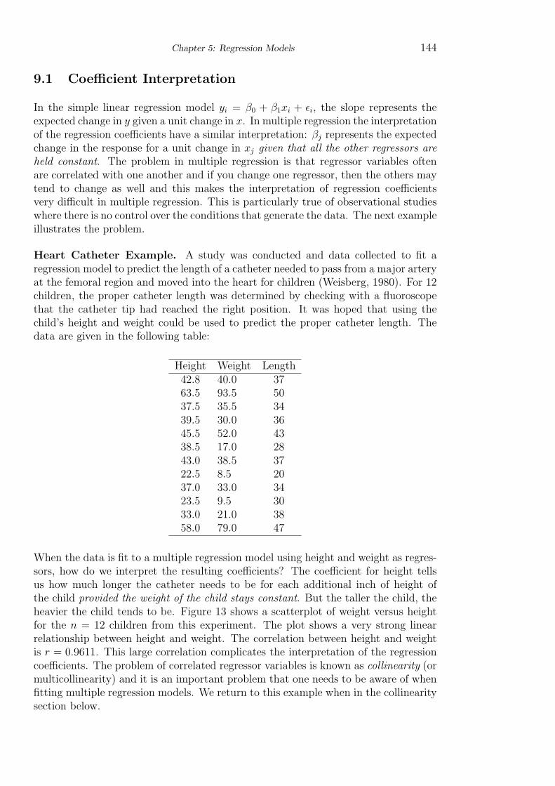
Heart Catheter Example. A study was conducted and data collected to fit aregression model to predict the length of a catheter needed to pass from a major arteryat the femoral region and moved into the heart for children (Weisberg, 1980). For 12children, the proper catheter length was determined by checking with a fluoroscopethat the catheter tip had reached the right position. It was hoped that using thechild’s height and weight could be used to predict the proper catheter length. Thedata are given in the following table:

Height Weight Length42.8 40.0 3763.5 93.5 5037.5 35.5 3439.5 30.0 3645.5 52.0 4338.5 17.0 2843.0 38.5 3722.5 8.5 2037.0 33.0 3423.5 9.5 3033.0 21.0 3858.0 79.0 47

When the data is fit to a multiple regression model using height and weight as regres-sors, how do we interpret the resulting coefficients? The coefficient for height tellsus how much longer the catheter needs to be for each additional inch of height ofthe child provided the weight of the child stays constant. But the taller the child, theheavier the child tends to be. Figure 13 shows a scatterplot of weight versus heightfor the n = 12 children from this experiment. The plot shows a very strong linearrelationship between height and weight. The correlation between height and weightis r = 0.9611. This large correlation complicates the interpretation of the regressioncoefficients. The problem of correlated regressor variables is known as collinearity (ormulticollinearity) and it is an important problem that one needs to be aware of whenfitting multiple regression models. We return to this example when in the collinearitysection below.


Figure 13: A scatterplot of weight versus height for n = 12 children in an experimentused to predict the required length of a catheter to the heart based on the child’sheight and weight.

Fortunately, in designed experiments where the engineer has complete control over theregressor variables, data may be able to be collected in a fashion so that the estimatedregression coefficients are uncorrelated. In such situations, the estimated coefficientscan then be easily interpreted. To make this happen, one needs to choose the valuesof the regressors so that the off-diagonal terms in the (X ′X)−1 matrix (from (9))that correspond to covariances between estimated coefficients of the regressors are allzero.

Cobalt Example Continued. Let us return to model (13) and estimate the pa-rameters of the model. Using the data in the cobalt example, we can construct the


design matrix X in (17) and the response vector y as:

X =

1 0.6 2001 0.6 2501 0.6 4001 0.6 5001 0.6 6001 1.0 2001 1.0 2501 1.0 4001 1.0 5001 1.0 6001 2.6 2001 2.6 2501 2.6 4001 2.6 5001 2.6 6001 2.8 2001 2.8 2501 2.8 4001 2.8 5001 2.8 600

y =

90.682.758.743.225.0127.1112.319.617.89.153.152.043.442.431.640.937.927.527.319.0

.

The least squares estimates of the parameters are given by β = (β0, β1, β2)′ where

β = (X ′X)−1X ′y

=

20 35 780035 79.8 136507800 13650 3490000

−1 961.2

1471.8309415

=

124.8788−11.3369−0.1461

.

The matrix computations are tedious, but software packages like Matlab can performthese for us. Nonetheless, it is a good idea to understand exactly what it is thecomputer software packages are computing for us when we feed data into them. Themean squared residual for this data is σ2 = MSres = 1754.69768 and the estimatedcovariance matrix of the estimated coefficients is

σ2(X ′X)−1 =

246.8702 −41.9933 −0.3875−41.9933 23.9962 0.0000−0.3875 0.0000 0.00099

.

Note that this was a well-designed experiment because the estimated coefficients forCobalt contents (β1) and Temperature (β2) are uncorrelated – the covariance betweenthem is zero as can be seen in the covariance matrix.


10 Analysis of Variance (ANOVA) for Multiple

Regression

Because there are several regression parameters in the multiple regression model (15),a formal test can be conducted to see if the response depends on any of the regressorvariables. That is, we conduct a single test of the hypothesis:

H0 : β1 = β2 = · · · βk = 0

versus

Ha : not all βj’s are zero.

The basic idea behind the testing procedure is to partition all the variability in theresponse into two pieces: variability due to the regression relation and variability dueto the random error term. This is why the procedure is called Analysis of Variance(ANOVA). The total variability in the response is represented by the total sums ofsquares (SSyy):

SSyy =n∑

i=1

(yi − y)2.

We have already defined the residual sum of squares:

SSres =n∑

i=1

(yi − yi)2.

We can also define the Regression Sum of Squares (SSreg):

SSreg =n∑

i=1

(yi − y)2

which represents the variability in the yi’s explained by the multiple regression model.Note that for an individual measurement

(yi − y) = (yi − yi) + (yi − y).

If we square both sides of this equation and sum over all n observations, we will getSSyy on the left-hand side. On the right-hand side (after doing some algebra) we willget SSres + SSreg only because the cross product terms sum to zero. This gives usthe well-known variance decomposition formula:

SSyy = SSreg + SSres. (18)

If all the βj’s are zero, then the regression model will explain very little of the variabil-ity in the response in which case SSreg will be small and SSres will be large, relativelyspeaking. The ANOVA test then simply compares these components of variance witheach other. However, in order to make the sums of squares comparable, we need tofirst divide each sum of squares by its respective degrees of freedom. The degrees


of freedom for the regression sum of squares is simply the number of β’s (for theintercept plus k regressors) in the model minus one:

dfreg = k.

The Mean Square for Regression is

MSreg =SSreg

k.

We have already defined the mean square for residuals:

MSres =SSres

n− k − 1

where the degrees of freedom for the residual sum of squares is the total sample sizeminus the number of β’s (k + 1):

dfres = n− k − 1.

The ANOVA test statistic is the ratio of the mean squares, which is denoted by F :

F =MSreg

MSres

. (19)

Assuming that the errors in the model (15) are independent and follow a normaldistribution, then the test statistic F follows an F-distribution on k numerator degreesof freedom and n − k − 1 denominator degrees of freedom. If the null hypothesis istrue (i.e. all βj’s equal zero), then F takes the value one on average. However, if thenull hypothesis is false, then the regression mean square tends to be larger than theerror mean square and F will be larger than one on average. Therefore, the F -testrejects the null hypothesis for large values of F . How large does F have to be? If thenull hypothesis is true, then the F test statistic follows an F distribution. Therefore,we use critical values from the F -distribution to determine the critical region for theF -test which can be looked up in an F -table (see pages 202–204 in the Appendix).

For a simple linear regression model yi = β0 + β1xi + ϵi, we used a t-test to testH0 : β1 = 0 versus Ha : β1 = 0. One can also perform an ANOVA F -test of thishypothesis and in fact, the two tests are equivalent. One can show with a littlealgebra that the square of the t-test statistic is equal to the ANOVA F -test statisticin a simple linear regression, i.e. t2 = (β1/σβ1

)2 = F .

Example continued... Returning to the multiple regression example on the effect ofcobalt contents and temperature on surface area, there were k = 2 regressor variablesused to predict surface area. If we test H0 : β1 = β2 = 0, our F -test statistic willbe compared with an F -critical value on k = 2 numerator degrees of freedom andn − k − 1 = 20 − 2 − 1 = 17 denominator degrees of freedom. This critical value isdenoted Fk,n−k−1,α where α is the significance level. Using α = 0.05, we can look upthe critical value in the F table (page 203) and find F2,17,.05 = 3.59. From the data,we compute that SSreg = 11947 and therefore MSreg = 12310/2 = 5973.43416. Also,SSres = 7567.19968 and MSres = 7567.19968/3 = 445.12939. The F -test statistic


comes out to be F = MSreg/MSres = 5973.43416/445.12939 = 13.42 which exceedsthe α = 0.05 critical value indicating that we reject H0 and conclude that β1 and β2

are not both zero. The results of the ANOVA F test are usually summarized in anANOVA table like the one below which was generated using the popular statisticalSAS software package:

Analysis of Variance

Sum of Mean

Source DF Squares Square F Value Pr > F

Model 2 11947 5973.43416 13.42 0.0003

Error 17 7567.19968 445.12939

Corrected Total 19 19514

In this ANOVA table, the Corrected Total sum of squares is SSyy. Note that addingthe Model and Error sum of squares gives the corrected total sum of squares: 11947+7567.19968 = 19514 (rounded to the nearest integer) showing the variance decom-position given in (18). Likewise, the model and error degrees of freedom add up toequal the corrected total degrees of freedom: 2 + 17 = 19 = n − 1. Finally, the lastcolumn of the ANOVA table gives the p-value of the test of p = 0.0003. Because thep-value is less than α = 0.05 we reject the null hypothesis. In fact, the p-value is verysmall indicating very strong evidence that at least one of the regression coefficientsdiffers from zero.

Once we have determined that at least one of the coefficients is non-zero, typicallyt-tests are conducted for the individual coefficients in the model:

H0 : βj = 0 versus Ha : βj = 0

for j = 1, . . . , k. The test statistics for each of these hypotheses is given by a t-teststatistic of the form

t =βj

σβj

where the σβjare found by taking the square roots of the diagonal elements of the

σ2(X ′X)−1 covariance matrix. Recall that the square root of the diagonal terms inσ2(X ′X)−1 are the estimated standard errors σβj

of the estimated regression coeffi-

cients. The t-statistics follow a t-distribution on n − k − 1 degrees of freedom (i.e.the residual degrees of freedom) when the null hypothesis is true. The following tablegenerated by SAS summarizes the tests for individual coefficients:

Parameter Estimates


Parameter Standard

Variable DF Estimate Error t Value Pr > |t|

Intercept 1 124.87880 15.71210 7.95 <.0001

cobalt 1 -11.33693 4.89859 -2.31 0.0334

temp 1 -0.14610 0.03152 -4.63 0.0002

This table gives the results of two-tailed test of whether or not the regression coeffi-cients are zero or not. The last column gives the p-values, all of which are less thanα = 0.05 indicating that both the cobalt content and the temperature are signifi-cant in modeling the surface area of the hydroxide catalyst. Because the experimentwas designed so that the estimated slope parameters for cobalt and temperature areuncorrelated, the interpretation of the coefficients is made easier. Note that bothcoefficients are negative indicating that increasing cobalt content and temperatureresults in lower surface area on average. The intercept of the model does not have aclear interpretation in this example because data was not collected at values of cobaltand temperature near zero.

It is possible to test more general hypotheses for individual regression coefficientssuch as H0 : βj = βj0 for some hypothesized value βj0 of the jth regression coefficient.The t-test statistic then becomes

t =βj − βj0

σβj

and the alternative hypothesis can be one-sided or two-sided.

Individual confidence intervals can be obtained for the regression coefficients usingthe formula as in the case of a simple linear regression model:

βj ± tα/2σβj.

However, individual confidence regions can be misleading when the estimated coef-ficients are correlated. A better method is to determine a joint confidence region.

11 Confidence Ellipsoids

In Chapter 4, the concept of a confidence region was introduced when estimators ofinterest are correlated with one another. In multiple regression the estimated coef-ficients are often correlated. Forming confidence intervals for individual regressioncoefficients can be misleading when considering more than one coefficient as in mul-tiple regression. The reason for this is that the region formed by two confidenceintervals is the Cartesian product forming a rectangle. If the estimated coefficientsare correlated, then some points in the confidence rectangle may not be plausiblevalues for the regression coefficients. We illustrate this idea below.


Figure 14: A 95% confidence ellipse for the regression coefficients β1 and β2 for cobaltcontent and temperature.

The following formula (e.g. see Johnson and Wichern, 1998, page 285) defines aconfidence ellipsoid in the regression setting: A 100(1− α)% confidence region for βis given by the set of β ∈ ℜk+1 that satisfy

(β − β)′(X ′X)(β − β) ≤ (k + 1)MSresFk+1,n−k−1,α.

The confidence region described by this inequality is an elliptical shaped region (seeChapter 4). In the previous example, if we want a confidence region for only (β1, β2)

′,the coefficients of cobalt content and temperature, the confidence region is given bythe set of (β1, β2)

′ ∈ ℜ2 satisfying the following inequality:

(β1 − β1, β2 − β2)[(0 1 00 0 1

)(X ′X)−1

0 01 00 1

]−1(β1 − β1

β2 − β2

)≤ 2MSresF2,n−k−1,α.

Figure 14 shows a 95% confidence ellipse for β1 and β2 in this example.

The major and minor axes of the confidence ellipse in Figure 14 are parallel to theβ1 and β2 axes because the estimates of these parameters are uncorrelated due to thedesign of the experiment. The estimators of the regression coefficients will not alwaysbe uncorrelated, particularly with observational data. The next example illustratesan experimental data set where the regression coefficients are correlated.

Hald Cement Data Example. An experiment was conducted to measure the heatfrom cement based on differing levels of the ingredients that make up the cement. Thisis the well-known Hald cement data (Hald 1932) which has been used to illustrateconcepts from multiple regression. The data are in the following table:


Amount of Amount of Amount of Amount of Heattricalcium tricalcium tetracalcium dicalcium evolvedaluminate silicate alumino ferrite silicate calories per gramx1 x2 x3 x4 y78.5 7.0 26.0 6.0 60.074.3 1.0 29.0 15.0 52.0104.3 11.0 56.0 8.0 20.087.6 11.0 31.0 8.0 47.095.9 7.0 52.0 6.0 33.0109.2 11.0 55.0 9.0 22.0102.7 3.0 71.0 17.0 6.072.5 1.0 31.0 22.0 44.093.1 2.0 54.0 18.0 22.0115.9 21.0 47.0 4.0 26.083.8 1.0 40. 23.0 34.0113.3 11.0 66.0 9.0 12.0109.4 10.0 68.0 8.0 12.0

A “full” model would incorporate all the regressor variables:

yi = β0 + β1xi1 + β2xi2 + β3xi3 + β4xi4 + ϵi.

One of the goals of this study was to determine the best “reduced” model that usedonly a subset of the regressors. In this example, the regressor variables are correlatedwith one another. If we consider a model with regressors x1 and x2 say, then adding x3

to the model may not provide much additional information. In statistical modeling,an important principal is the principal of parsimony which means to use the simplestmodel possible that still adequately explains the data. More complicated models (e.g.more regressor variables) can have undesirable properties such as unstable parameterestimates.

In order to illustrate further the concept of confidence ellipses, we shall fit a multipleregression of y on x1 and x2 only. The ANOVA table from running SAS is


Sum of Mean


Model 2 3175.37558 1587.68779 85.07 <.0001

Error 10 186.62442 18.66244

Corrected Total 12 3362.00000

The F -test statistic equals 85.07 and the associated p-value is less than 0.0001 indi-cating that there is very strong statistical evidence that at least one of the coefficientsfor x1 and x2 are non-zero. The R2 from this fitted model is R2 = 0.9445 indicatingthat most of the variability in the response is explained by the regression relationshipwith x1 and x2. The estimated parameters, standard errors and t-test for equality tozero are tabulated below:


Parameter Estimates

Parameter Standard


Intercept 1 160.08461 10.09097 15.86 <.0001

x1 1 -1.53258 0.12143 -12.62 <.0001

x2 1 2.16559 0.31054 6.97 <.0001

Both parameter estimates differ significantly from zero as indicated by the p-values< 0.0001 for x1 and x2. The estimated coefficient for x1 (amount of tricalcium alu-minate) is β1 = −1.53258 and the estimated coefficient for x2 (Amount of tricalciumsilicate) is β2 = 2.16559 which seems to indicate that the amount of heat produceddecreases with increasing levels of tricalcium aluminate and the amount of heat in-creases with increasing levels of tricalcium silicate. However, x1 and x2 are correlatedwith one another (sample correlation r = 0.7307) and thus, we cannot easily interpretthe coefficients due to this correlation. The estimated covariance matrix of (β1, β2)

′

is

σ(X ′X)−1 =

101.8276 -1.2014 1.9098-1.2014 0.0148 -0.02761.9098 -0.0276 0.0964

indicating that β1 and β2 are negatively correlated with one another as well (sincethe covariance between them is −0.0276). Figure 15 shows a 95% confidence ellipsefor the coefficients β1 and β2. Also shown is a rectangular confidence region obtainedby taking the Cartesian product of individual confidence intervals for β1 and β2 sep-arately. The fact that the ellipse tilts downward from left to right indicates that theestimated coefficients are negatively correlated. In addition, points that lie in therectangular confidence region but not inside the ellipse are not really plausible valuesfor the coefficients because they do not lie inside the elliptical confidence region. Toillustrate this point, the symbol × in the plot lies inside the confidence rectangle andwould seem to be a plausible value for (β1, β2)

′. However, since this point lies outsidethe confidence ellipse, it is not a plausible value with 95% confidence.

12 Polynomial Regression.

A special case of multiple regression is polynomial regression. If a scatterplot of yversus x indicates a nonlinear relationship, then fitting a straight line is not appropri-ate. For example, the response y may be a quadratic function of x. If the functionalrelationship between x and y is unknown, then a Taylor series approximation mayprovide a reasonable way of modeling the data which would entail fitting a polynomialto the data. The polynomial regression model can be expressed as

yi = β0 + β1xi + β2x2i + · · ·+ βkx

ki + ϵi. (20)

To see that (20) is a special case of the multiple regression model, simply define themultiple regressor variables to be x1 = x, x2 = x2, . . . , xk = xk. Although (20) is


Figure 15: A 95% confidence ellipse for the regression coefficients β1 and β2 for haldcement data.

a nonlinear function of x, it is nonetheless considered a linear model because it isexpressed as a linear function of the parameters β0, β1, . . . , βk.

Least squares estimators of the parameters in (20) can be found exactly as for othermultiple regression models by computing β = (X ′X)−1X ′y. The next exampleillustrations the computations involved.

Example. An experiment was conducted to study the daily production of sulfu-ric acid (in tons) and its dependence on the temperature (in Celcius) at which theproduction process was run (Graybill and Iyer, page 461). The data is in the tablebelow:

Temp Acid100 1.93125 2.22150 2.85175 2.69200 3.01225 3.82250 3.91275 3.65300 3.71325 3.40350 3.71375 2.57400 2.71

A scatterplot sulfuric acid amount versus temperature is shown in Figure 16. Clearly


Figure 16: Sulfuric Acid y versus Temperature x.

the relationship between acid and temperature is nonlinear. One of the goals of thestudy is to determine the optimal temperature that will result in the highest yieldof sulfuric acid. Figure 16 suggests that a quadratic model may fit the data well:yi = β0 + β1xi + β2x

2i + ϵi. The design matrix for the quadratic model is

X =

1 x1 x2

1

1 x2 x22

......

...1 xn x2

n

=

1. 100 100001 125 156251 150 225001 175 306251 200 400001 225 506251 250 625001 275 756251 300 900001 325 1056251 350 1225001 375 1406251 400 160000

Figure 17 shows the scatterplot of the data along with the fitted quadratic curvey = −1.141878 + 0.035519x− 0.000065x2. In order to estimate the temperature thatproduces the highest yield of sulfuric acid, simply take the derivative of this quadraticfunction, set it equal to zero and solve for x.

One of the shortcomings of polynomial regression is that the fitted models can becomevery unstable when fitting higher order polynomials. The estimated covariance matrix


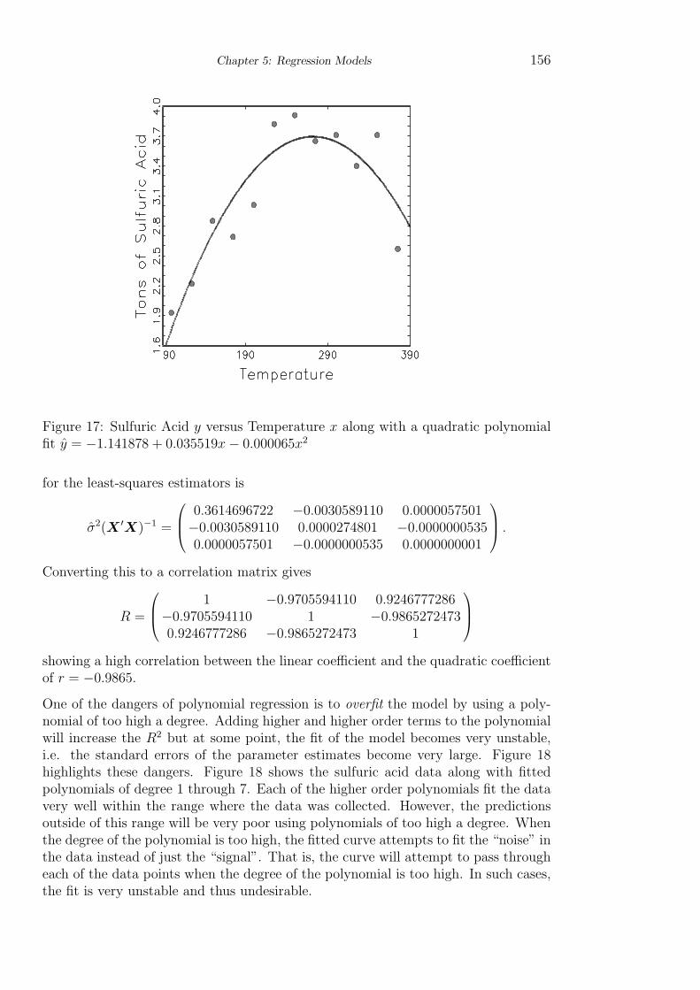
Figure 17: Sulfuric Acid y versus Temperature x along with a quadratic polynomialfit y = −1.141878 + 0.035519x− 0.000065x2

for the least-squares estimators is

σ2(X ′X)−1 =

0.3614696722 −0.0030589110 0.0000057501−0.0030589110 0.0000274801 −0.00000005350.0000057501 −0.0000000535 0.0000000001

.

Converting this to a correlation matrix gives

R =

1 −0.9705594110 0.9246777286−0.9705594110 1 −0.98652724730.9246777286 −0.9865272473 1

showing a high correlation between the linear coefficient and the quadratic coefficientof r = −0.9865.

One of the dangers of polynomial regression is to overfit the model by using a poly-nomial of too high a degree. Adding higher and higher order terms to the polynomialwill increase the R2 but at some point, the fit of the model becomes very unstable,i.e. the standard errors of the parameter estimates become very large. Figure 18highlights these dangers. Figure 18 shows the sulfuric acid data along with fittedpolynomials of degree 1 through 7. Each of the higher order polynomials fit the datavery well within the range where the data was collected. However, the predictionsoutside of this range will be very poor using polynomials of too high a degree. Whenthe degree of the polynomial is too high, the fitted curve attempts to fit the “noise” inthe data instead of just the “signal”. That is, the curve will attempt to pass througheach of the data points when the degree of the polynomial is too high. In such cases,the fit is very unstable and thus undesirable.


Figure 18: Polynomial fits of degrees 1 to 7 to the sulfuric data.

In order to determine the appropriate degree to use when fitting a polynomial, onecan choose the model that leads to the smallest residual mean square MSres. Theresidual sum of squares SSres gets smaller as the degree of the polynomial gets larger.However, each time we add another term to the model, we lose a degree of freedomfor estimating residual mean square. Recall that the residual mean square is definedby dividing the residual sum of squares by n− k− 1 where k equals the degree of thepolynomial (e.g. k = 2 for a quadratic model). The following table gives the R2 andMSres for different polynomial fits:

Degree R2 MSres

1 0.1877 0.37852 0.8368 0.08373 0.8511 0.08484 0.8632 0.08765 0.8683 0.09646 0.8687 0.11227 0.8884 0.1144

As seen in the table, the R2 increases with the degree of the polynomial. However,for polynomials of degree 3 and higher, the increase in R2 is very slight. The residualmean square is smallest for the quadratic fit indicating that the quadratic fit is bestaccording to this criteria.


Figure 19: 3-D plot of the heart catheter data.

13 Collinearity

One of the most serious problems in a multiple regression setting is (multi)collinearitywhen the regressor variables are correlated with one another. Collinearity causesmany problems in a multiple regression model. One of the main problems is thatif collinearity is severe, the estimated regression coefficients are very unstable andcannot be interpreted. In the heart catheter data set described above, the heightand weight of the children were highly correlated (r = 0.9611). Figure 19 showsa 3-dimensional plot of the height and weight as well as the response variable y =length. The goal of the least-squares fitting procedure is to determine the best-fittingplane through these points. However, the points lie roughly along a straight line inthe height-weight plane. Consequently, fitting the regression plane is analogous totrying to build a table when all the legs of the table lie roughly in a straight line. Theresult is a very wobbly table. Ordinarily, tables are designed so that the legs are farapart and spread out over the surface of the table. When fitting a regression surfaceto highly correlated regressors, the resulting fit is very unstable. Slight changes inthe values of the regressor variables can lead to dramatic differences in the estimatedparameters. Consequently, the standard errors of the estimated regression coefficientstend to be inflated. In fact, it is quite common for none of the regression coefficientsto differ significantly from zero when individual t-tests are computed for regressioncoefficients. Additionally, the regression coefficients can have the wrong sign – onemay obtain a negative slope coefficient when instead a positive coefficient is expected.


Heart Catheter Example. A multiple regression was used to model the length ofthe catheter (y) with regressors height (x1) and weight (x2):

yi = β0 + β1xi1 + β2xi2 + ϵi.

The ANOVA table (from SAS) is below:


Sum of Mean


Model 2 607.18780 303.59390 21.27 0.0004

Error 9 128.47887 14.27543

Corrected Total 11 735.66667

The overall F -test indicates that at least one of the slope parameters β1 and/orβ2 differs significantly from zero (p-value = 0.0004). Furthermore, the coefficientof determination is R2 = 0.8254 indicating that height and weight explain most ofthe variability in the required catheter length. However, the parameter estimates,standard errors, t-test statistics and p-values shown below indicate that neither β1

nor β2 differ significantly from zero.

Parameter Estimates

Parameter Standard


Intercept 1 20.37576 8.38595 2.43 0.0380

height 1 0.21075 0.34554 0.61 0.5570

weight 1 0.19109 0.15827 1.21 0.2581

The apparent paradox is that the overall F -test says at least one of the coefficientsdiffers from zero whereas the individual t-tests says neither differ from zero is dueto the collinearity problem. This phenomenon is quite common when collinearity ispresent. A 95% confidence ellipse for the estimated regression coefficients of heightand weight shown in Figure 20 shows that the estimated regression coefficients arehighly correlated because the confidence ellipse is quite eccentric.

Another major problem when collinearity is present is that the fitted model will notbe able to produce reliable predictions for values of the regressors away from the rangeof the regressor values. If the data changes just slightly, then the predicted valuesoutside the range of the data can change dramatically when collinearity is a present– just think of the wobbly table analogy.

In a well designed experiment, the values of the regressor variables will be orthog-onal which means that the covariances between estimated coefficients will be zero.


Figure 20: A 95% confidence ellipse for the coefficients of height and weight in theheart catheter example.

Figure 21: 3-D plot of orthogonal regressor variables.


Figure 21 illustrates an orthogonal design akin to the usual placement of legs on atable.

There are many solutions to the collinearity problem:

• The easiest solution is to simply drop regressors from the model. In the heartcatheter example, height and weight are highly correlated. Therefore, if we fita model using only height as a regressor, then we do not gain much additionalinformation by adding weight to the model. In fact, if we fit a simple linearregression using only height as a regressor, the coefficient of height is highlysignificant (p-value < 0.0001) and the R2 = 0.7971 is just slightly less than ifwe had used both height and weight as regressors. (Fitting a regression usingonly weight as a regressor yields an R2 = 0.8181.) When there are severalregressors, the problem becomes one of trying to decide upon which subset ofregressors works best and which regressors to throw out. Often times, theremay be several different subsets of regressors that work reasonably well.

• Collect more data with the goal of spreading around the values of the regres-sors so they do not form the “picket fence” type pattern as seen in Figure 19.Collecting more data may not solve the problem in situations where the exper-imenter has no control over the relationships between the regressors, as in theheart catheter example.

• Biased regression techniques such as ridge regression and principal componentregression. Details can be found in advanced textbooks on regression. Thesemethods are called biased because the resulting slope estimators are biased.The tradeoff is that the resulting estimators will be more stable.

In polynomial regression, collinearity is a very common problem when fitting higherorder polynomials and the resulting least-squares estimators tend to be very unsta-ble. Centering the regressor variable x at its mean (i.e. using xi − x instead of xi)helps alleviate this problem to some extent. Another solution is to fit a polynomialregression using orthogonal polynomials (details of this method can also be found inmany advanced texts on regression analysis).

14 Additional Notes on Multiple Regression

One can compute confidence intervals for a mean response or prediction intervals fora predicted response as was done in the simple linear regression model. The exactsame formulas (10) and (11) apply as in the simple linear regression model exceptthe degrees of freedom needs to correspond to the residual mean square degrees offreedom. Most statistical software packages can compute these intervals.

The problem of checking the adequacy of the multiple regression model is considerablytougher than in simple linear regression because we cannot plot the full data set due tothe high dimension of the data. Nonetheless, a plot of residuals versus fitted values isstill useful in order to determine the appropriateness of the model. If structure exists


in the residual plot, then the model needs to be reconsidered. Perhaps quadraticterms and interaction terms such as x1 ·x2 need to be incorporated into the model. Auseful diagnostic tool is to also plot residuals versus each of the regression variablesto see if any structure shows up in these plots as well.

As indicated by the Anscombe data set (Figure 12), the fitted regression surface canbe highly influenced by just a few observations. In the Anscombe data set, it waseasy to see the offending point, but in a multiple regression setting, it can be difficultto determine which, if any, points may be strongly effecting the fit of the regression.There are several diagnostic tools to help with this problem and advanced textbooksin regression analysis discuss these tools.

15 Advanced Topics in Regression

Regression analysis is a very wide topic and we have introduced the basic ideas sofar in this chapter. There are several additional regression topics that are used byengineers that will be briefly mentioned here.

15.1 Nonlinear Models

First, some terminology: it is important to note that up to this point in this chapter,the regression models such as (13) and (14) are both examples of what are calledlinear models because the response y is a linear function of the parameters (i.e., theβ’s) even though (14) has quadratic terms (such as x2

i1 etc.). This terminology maybe a bit confusing since a model with quadratic terms is still called a linear model.Other examples of linear models are

yi = β0 + β1 log(xi1) + ϵi

andyi = β0 + β1(xi1/x

2i2) + ϵi

because once again, these equations are linear in terms of the βj’s. In each of thesecases, we can find the least squares estimators of the βj’s by simply applying for-mula (16). That is, there exists a closed-form solution for the least-squares estima-tors.

A nonlinear regression model is one where the response is related to the model param-eters in a nonlinear fashion. These types of models are very common in engineeringapplications. A couple of nonlinear regression model examples are

yi = β1e−β2xi1 + ϵi

and

yi =β0 + β1xi1

β2xi2 + β3xi3

+ ϵi.

Neither of these two models are linear in the parameters and thus they are not linearmodels. To find the least squares estimators in such cases one can either try to find a


transformation that will linearize the relationship (such as a log-transformation in thefirst example) or use an iterative algorithm (such as the Gauss-Newton algorithm) tofind the estimators because there does not exist a closed form solution to the leastsquares estimators as in the case of linear models. Most statistical software packageshave routines that will fit nonlinear regression models. The algorithms for nonlinearregression usually require specifying some initial guesses for the parameter values andone needs to be careful in choosing these initial values or else the iterative algorithmmay crash or go off in the wrong direction.

15.2 Nonparametric Regression

All of the regression models introduced up to this point impose a specific functionalrelationship between the response and the predictor(s) (e.g. straight line, quadratic,exponential, etc.). In many applications, the investigator may want to let the datadetermine the shape of the functional response. In this case, one can use a nonpara-metric regression approach. The idea behind some of approaches is to predict theresponse at a point x by taking a “local” average of the responses in a neighborhoodof values around x.

Another popular approach is to use what are called spline models where pieces ofpolynomials (usually cubic polynomials) are pieced together to form a smooth curve.

15.3 Logistic Regression

In Chapter 2, the binomial distribution was introduced. As we saw in that chapter,in many applications, the response of interest is binary (0 or 1) indicating a successor failure. For example, one may run an experiment at different temperatures andnote which ones result in a success or failure. A tragic example of this was the SpaceShuttle Challenger disaster that occurred on January 28, 1986 due to o-ring failureson that cold morning. In logistic regression, the idea is to model a binary responseas a function of one or more covariates (or predictors), like temperature.

If x denotes a predictor and y is a binary response, then in logistic regression wemodel the expected value of y given x. However, since y is binary, this expectationbecomes a conditional probability, which we can write p(x) = probability of successgiven x. Typically, the logistic regression model that is used is

p(x) =eβ0+β1x

1 + eβ0+β1x, (21)

which produces an “S” shaped regression curve usually. As with nonlinear regression,iterative algorithms are needed to estimate the logistic regression parameters.

Problems

1. Brownlee (1965) discusses an experiment looking at the oxidation of ammoniato nitric acid at a chemical plant. The response variable is the percentage of


unprocessed ammonia. The regressors are x1 = operation time, x2 = temper-ature of the coolant, and x3 = acid concentration. n = 21 observations wereobtained.

Operation Time Coolant Temperature Acid Concentration Unprocessed %x1 x2 x3 y80 27 89 4280 27 88 3775 25 90 3762 24 87 2862 22 87 1862 23 87 1862 24 93 1962 24 93 2058 23 87 1558 18 80 1458 18 89 1458 17 88 1358 18 82 1158 19 93 1250 18 89 850 18 86 750 19 72 850 19 79 850 20 80 956 20 82 1570 20 91 15

Consider the following multiple regression model

yi = β0 + β1xi1 + β2xi2 + β3xi3 + ϵi.

a) The following computations were performed:

(X ′X)−1 =

13.452727 0.027339 −0.061961 −0.1593550.027339 0.001729 −0.003471 −0.000679−0.061961 −0.003471 0.012875 0.000001−0.159355 −0.000679 0.000001 0.002322

, and X ′y =

36823953832632189

.

Use these computations to compute β, the estimated regression coeffi-cients.

b) Write down the equation for the fitted regression equation.

c) Compute the fitted value y1 for the first observation as well as the firstresidual r1 = y1 − y1.

d) Here is an ANOVA table from the multiple regression model:



Source DF SS MS F P

Regression 3 1890.41 630.14 59.90 0.000

Error 17 178.83 10.52

Total 20 2069.24

Compute the coefficient of determination R2.

e) Compute 3 t-test statistics for testing if the regression coefficients β1, β2

and β3 differ significantly from zero. Which coefficients differ significantlyfrom zero (use α = 0.05 to make your decision for each test).

f) Another regression model was fit to the data by dropping out the acidconcentration regressor (x3). The ANOVA table from fitting a regressionusing only x1 and x2 is given here:

Source DF SS MS F P

Regression 1880.44 940.22 89.64 0.000

Error

Total 2069.24

Fill in the missing values for the degrees of freedom, the sum of squares forthe residuals and the MSE. What is the coefficient of determination R2

for this “reduced” model? How does it compare to the R2 from the “full”model using all three regressor variables?

2. An air mixture consists of oxygen and nitrogen only. Suppose an experiment isrun by varying the percentages of the air mixture and how it effects the strengthof a weld made using the air mixture. The following table gives the hypotheticaldata from this experiment:

Oxygen % (x1) Nitrogen % (x2) Strength (y)50% 50% 9340% 60% 8730% 70% 8020% 80% 72

a) Write down the design matrix X for fitting the model yi = β0 + β1xi1 +β2xi2 + ϵi.

b) Can you express the third column of X as a linear combination of the firsttwo columns?

c)) What goes wrong when we fit the above model? Running this model usingthe statistical software SAS gives the following message: “Model is not fullrank. Least-squares solutions for the parameters are not unique.” Whatdoes this mean?

d) Find the least-squares line for regressing y on x1 alone and regression y onx2 alone. How are the slope estimates related in these two models?


e) If you had to offer advice on how to fit a regression model to this data,what would you suggest be done?

References

Anscombe, F. J. (1973). Graphs in statistical analysis. The American Statistician27:17–21.

Brownlee, K. A. (1965). Statistical Theory and Methodology.

Graybill, F. A. and Iyer, H. K. (1994). Regression analysis: concepts and applications.Duxbury, Belmont, California.

Henderson, H. V. and Velleman, P. F. (1981). Building regression models interactively.Biometrics 37:391–411.

Johnson, R. A. and Wichern, D. W. (1998). Applied Multivariate Statistical Analysis.Prentice Hall, New Jersey.

Said, A., Hassan, E., El-Awad, A., El-Salaam, K., and El-Wahab, M. (1994). Struc-tural changes and surface properties of coxfe3−xo4 spinels. Journal of ChemicalTechnology and Biotechnology 60:161–170.

Weisberg, S. (1980). Applied Linear Regression. Wiley, New York.

Documents

Chapter 5. Regression Modelsthaddeus.tarpey/STT363chapter5.pdfChapter 5: Regression Models 118 April 9, 2013 ... we ﬁrst return to the very simple model introduced in Chapter 1 to