Embed Size (px)
Citation preview
Prof. Dr. Kai Carstensen and Prof. Dr. T. Wollmershäuser
New Keynesian Macroeconomics
Chapter 5: Monetary Policy Design in the New Keynesian
Model
Carstensen / Wollmershäuser, New Keynesian Macroeconomics, Slide 2
Monetary Policy Design
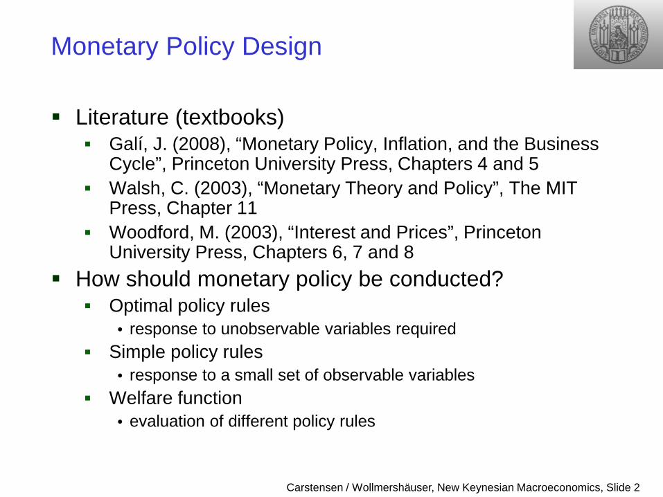
Literature (textbooks) Galí, J. (2008), “Monetary Policy, Inflation, and the Business
Cycle”, Princeton University Press, Chapters 4 and 5 Walsh, C. (2003), “Monetary Theory and Policy”, The MIT
Press, Chapter 11 Woodford, M. (2003), “Interest and Prices”, Princeton
University Press, Chapters 6, 7 and 8 How should monetary policy be conducted?
Optimal policy rules • response to unobservable variables required
Simple policy rules • response to a small set of observable variables
Welfare function • evaluation of different policy rules
Carstensen / Wollmershäuser, New Keynesian Macroeconomics, Slide 3
Monetary Policy Design
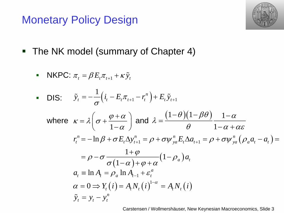
The NK model (summary of Chapter 4)
NKPC:
DIS:
where and
1π β π κ+= + t t t tE y
( )1 11 πσ + += − − − + n
t t t t t t ty i E r E y
( )
( ) ( )
1 1ln
1 11
n n n nt t t ya t t ya a t t
a t
r E y E a a a
a
β σ ρ σψ ρ σψ ρ
ϕρ σ ρσ α ϕ α
+ += − + ∆ = + ∆ = + − =
+= − −
− + +
1ϕ ακ λ σ
α+ = + −
( ) ( ) ( )10 αα −= ⇒ = =t t t t tY i A N i A N i= − n
t t ty y y
( )( )1 1 11
θ βθ αλθ α αε
− − −=
− +
1ln ln at t a t ta A Aρ ε−≡ = +
Carstensen / Wollmershäuser, New Keynesian Macroeconomics, Slide 4
Monetary Policy Design
Lucas critique “Given that the structure of an econometric model consists of
optimal decision rules of economic agents, and that optimal decision rules vary systematically with changes in the structure of series relevant to the decision maker, it follows that any change in policy will systematically alter the structure of econometric models.” • Lucas, R. (1976), “Econometric Policy Evaluation: A Critique”, in:
Brunner, K. and A. Meltzer, “The Phillips Curve and Labor Markets”, Carnegie-Rochester Conference Series on Public Policy, 1, New York: American Elsevier, pp. 19–46.
The introduction of rational expectations in macroeconomics in the middle of the 1970s represented a serious challenge for large-scale, backward-looking econometric models that were used for policy analysis.
Carstensen / Wollmershäuser, New Keynesian Macroeconomics, Slide 5
Monetary Policy Design
Lucas critique The observable reduced form of the economy can be
represented by 𝑌𝑡+1 = 𝐹 𝑌𝑡,𝑋𝑡,𝜃,𝑢𝑡 , where 𝑌𝑡 is a vector of economic variables, 𝑋𝑡 is a vector of policy instruments, 𝜃 is a parameter vector, and 𝑢𝑡 represents random shocks.
A policy rule for setting the policy instrument can be given by 𝑋𝑡 = 𝐺 𝑌𝑡,𝑔, 𝜉𝑡 , where 𝑔 is a vector of policy rule coefficients, and 𝜉𝑡 is a random shock.
Lucas argued that “scientific, quantitative policy evaluation” required comparing alternative policy rules, that is, examining changes in 𝑔 while taking into account agents’ expectations of future policy actions.
Carstensen / Wollmershäuser, New Keynesian Macroeconomics, Slide 6
Monetary Policy Design
Lucas critique He stressed that, “A change in policy [in 𝑔] affects the
behavior of the system in two ways: first by altering the time series behavior of [𝑋𝑡]; second by leading to modification of the behavioral parameters [𝜃(𝑔)] governing the rest of the system.” • The first effect is the obvious direct influence of the change in the
policy rule on the dynamics of the system. • The second expectational effect captures the fact that changes in
the policy rule should alter agents’ expectations of the future and, hence, change the reduced-form dynamics of the economy.
This sensitivity of the reduced form to the expectational effects of structural policy changes is the essence of the Lucas critique.
Carstensen / Wollmershäuser, New Keynesian Macroeconomics, Slide 7
Monetary Policy Design
Lucas critique Because the parameters of reduced-form models are not
structural, i.e. not policy-invariant, they would necessarily change whenever policy was changed. • Lucas argued that changes in policy have an immediate effect on
agents’ decision rules since they are inherently forward-looking and adapt to the effects of the new policy regime.
• An important corollary of this argument is that any policy evaluation based on backward-looking macroeconomic models is misleading whenever such policy shifts occur.
The Lucas critique suggests that if we want to predict the effect of a policy experiment, we should model and estimate the “deep parameters” (relating to preferences, technology and resource constraints) that govern individual behavior.
Carstensen / Wollmershäuser, New Keynesian Macroeconomics, Slide 8
Monetary Policy Design
Lucas critique We can then predict what individuals will do, taking into
account the change in policy, and then aggregate the individual decisions to calculate the macroeconomic effects of the policy change. • Changes in policy will have effects on the reduced-form dynamics
of the model. • This is important for normative policy analysis.
The Lucas critique encouraged macroeconomists to build microfoundations for their models. • Macro models of the New Keynesian type are microfounded.
Carstensen / Wollmershäuser, New Keynesian Macroeconomics, Slide 9
Monetary Policy Design
Contents of Chapter 5 a. Sources of suboptimality b. Optimal monetary policy I c. Simple policy rules I d. The welfare function e. Monetary policy tradeoffs f. Optimal monetary policy II (discretion versus commitment) g. Simple policy rules II h. Monetary policy under uncertainty
Carstensen / Wollmershäuser, New Keynesian Macroeconomics, Slide 10
Monetary Policy Design
Sources of suboptimality The New Keynesian model departs from a classical monetary
model, which corresponds to a conventional RBC model with a monetary sector, in two important aspects:
1. Monopolistic competition • Prices are set by firms that optimize their profit. • They are not determined by an anonymous Walrasian
auctioneer who is trying to clear competitive markets at once. 2. Nominal rigidities (sticky prices)
• Firms are subject to some constraints on the frequency with which they can adjust their prices.
In the event of macroeconomic disturbances both features together lead to deviations of the adjustment process from the optimal path that is implied by the frictionless classical monetary economy.
Carstensen / Wollmershäuser, New Keynesian Macroeconomics, Slide 11
Sources of suboptimality
Efficient allocation (first-best, classical monetary model) perfect competition
Flexible price equilibrium (second-best) monopolistic competition flexible prices
Staggered price equilibrium monopolistic competition staggered prices
Carstensen / Wollmershäuser, New Keynesian Macroeconomics, Slide 12
Sources of suboptimality
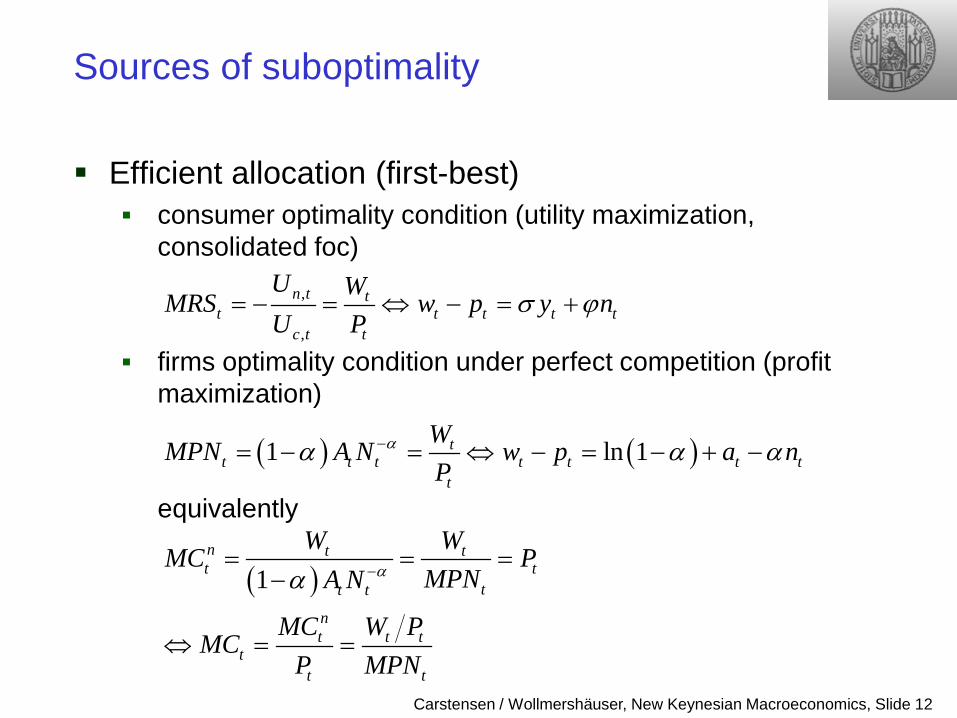
Efficient allocation (first-best) consumer optimality condition (utility maximization,
consolidated foc)
firms optimality condition under perfect competition (profit maximization)
equivalently
,
,
n t tt t t t t
c t t
U WMRS w p y n
U Pσ ϕ= − = ⇔ − = +
( ) ( )1 ln 1tt t t t t t t
t
WMPN A N w p a n
Pαα α α−= − = ⇔ − = − + −
( )1n t tt t
tt t
nt t t
tt t
W WMC P
MPNA N
MC W PMC
P MPN
αα −= = =−
⇔ = =
Carstensen / Wollmershäuser, New Keynesian Macroeconomics, Slide 13
Sources of suboptimality
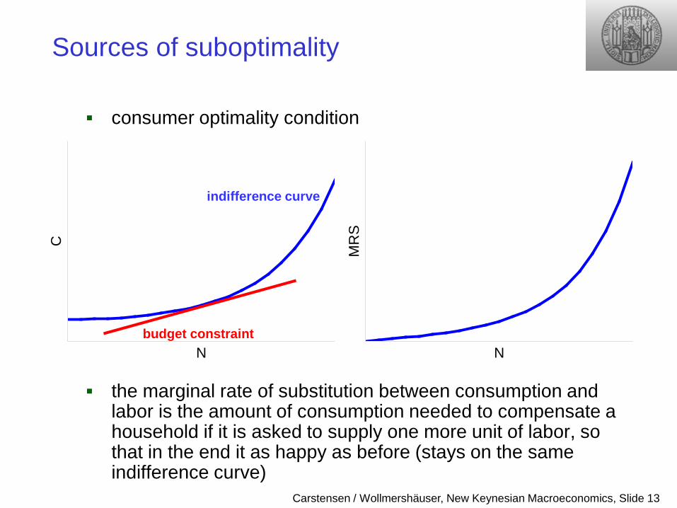
consumer optimality condition
the marginal rate of substitution between consumption and labor is the amount of consumption needed to compensate a household if it is asked to supply one more unit of labor, so that in the end it as happy as before (stays on the same indifference curve)
N
C
indifference curve
NM
RS
budget constraint
Carstensen / Wollmershäuser, New Keynesian Macroeconomics, Slide 14
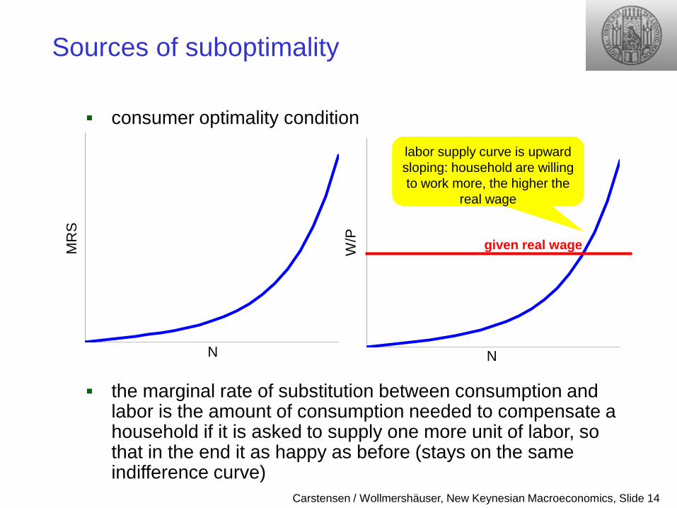
consumer optimality condition
the marginal rate of substitution between consumption and labor is the amount of consumption needed to compensate a household if it is asked to supply one more unit of labor, so that in the end it as happy as before (stays on the same indifference curve)
labor supply curve is upward sloping: household are willing to work more, the higher the
real wage
Sources of suboptimality M
RS
N W
/P
N
given real wage
Carstensen / Wollmershäuser, New Keynesian Macroeconomics, Slide 15
Sources of suboptimality
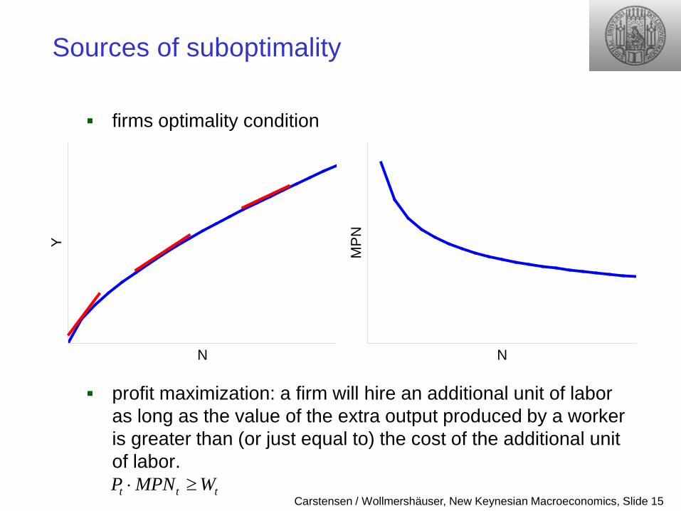
firms optimality condition
profit maximization: a firm will hire an additional unit of labor as long as the value of the extra output produced by a worker is greater than (or just equal to) the cost of the additional unit of labor.
N
Y
NM
PN
t t tP MPN W⋅ ≥
Carstensen / Wollmershäuser, New Keynesian Macroeconomics, Slide 16
Sources of suboptimality
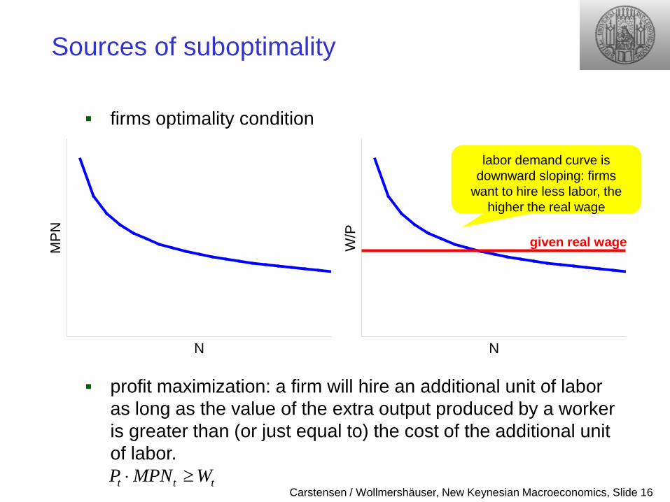
firms optimality condition
profit maximization: a firm will hire an additional unit of labor as long as the value of the extra output produced by a worker is greater than (or just equal to) the cost of the additional unit of labor.
t t tP MPN W⋅ ≥
N
MP
N
NW
/P
labor demand curve is downward sloping: firms
want to hire less labor, the higher the real wage
given real wage
Carstensen / Wollmershäuser, New Keynesian Macroeconomics, Slide 17
Sources of suboptimality
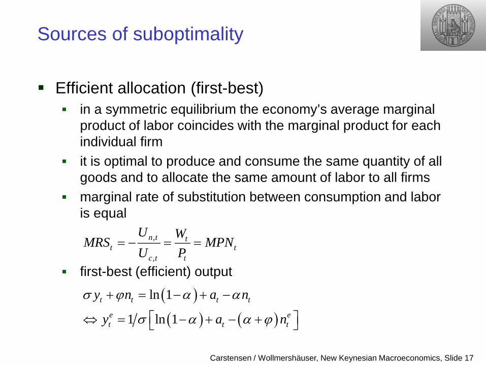
Efficient allocation (first-best) in a symmetric equilibrium the economy’s average marginal
product of labor coincides with the marginal product for each individual firm
it is optimal to produce and consume the same quantity of all goods and to allocate the same amount of labor to all firms
marginal rate of substitution between consumption and labor is equal
first-best (efficient) output
,
,
n t tt t
c t t
U WMRS MPN
U P= − = =
( )( ) ( )
ln 1
1 ln 1t t t t
e et t t
y n a n
y a n
σ ϕ α α
σ α α ϕ
+ = − + −
⇔ = − + − +
Carstensen / Wollmershäuser, New Keynesian Macroeconomics, Slide 18
Sources of suboptimality
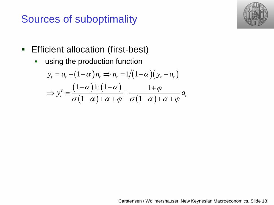
Efficient allocation (first-best) using the production function
( ) ( )( )( ) ( )( ) ( )
1 1 1
1 ln 1 11 1
t t t t t t
et t
y a n n y a
y a
α α
α α ϕσ α α ϕ σ α α ϕ
= + − ⇒ = − −
− − +⇒ = +
− + + − + +
Carstensen / Wollmershäuser, New Keynesian Macroeconomics, Slide 19
Sources of suboptimality
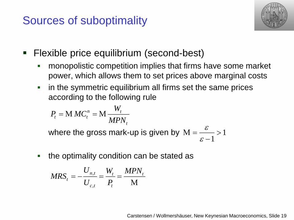
Flexible price equilibrium (second-best) monopolistic competition implies that firms have some market
power, which allows them to set prices above marginal costs in the symmetric equilibrium all firms set the same prices
according to the following rule
where the gross mark-up is given by
the optimality condition can be stated as
n tt t
t
WP MC
MPN= Μ = Μ
11
εε
Μ = >−
,
,
n t t tt
c t t
U W MPNMRS
U P= − = =
Μ
Carstensen / Wollmershäuser, New Keynesian Macroeconomics, Slide 20
Sources of suboptimality
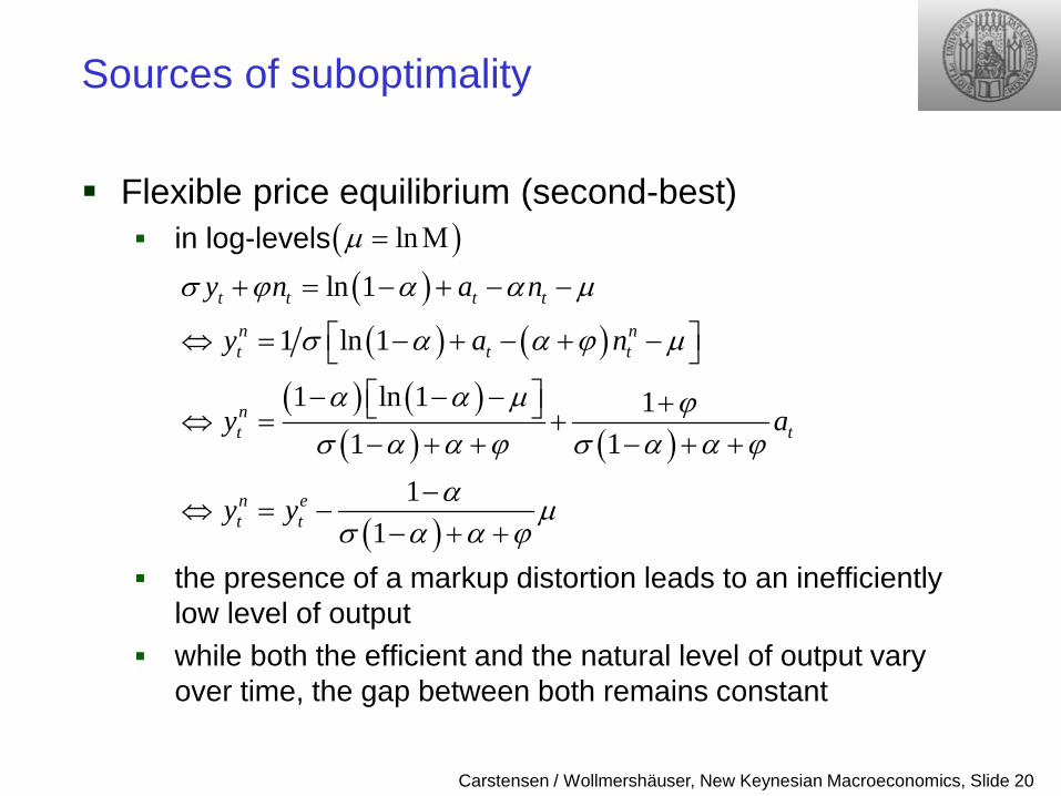
Flexible price equilibrium (second-best) in log-levels
the presence of a markup distortion leads to an inefficiently low level of output
while both the efficient and the natural level of output vary over time, the gap between both remains constant
( )( ) ( )
( ) ( )( ) ( )
( )
ln 1
1 ln 1
1 ln 1 11 1
11
t t t t
n nt t t
nt t
n et t
y n a n
y a n
y a
y y
σ ϕ α α µ
σ α α ϕ µ
α α µ ϕσ α α ϕ σ α α ϕ
α µσ α α ϕ
+ = − + − −
⇔ = − + − + − − − − + ⇔ = +− + + − + +
−⇔ = −
− + +
( )lnµ = Μ
Carstensen / Wollmershäuser, New Keynesian Macroeconomics, Slide 21
Sources of suboptimality
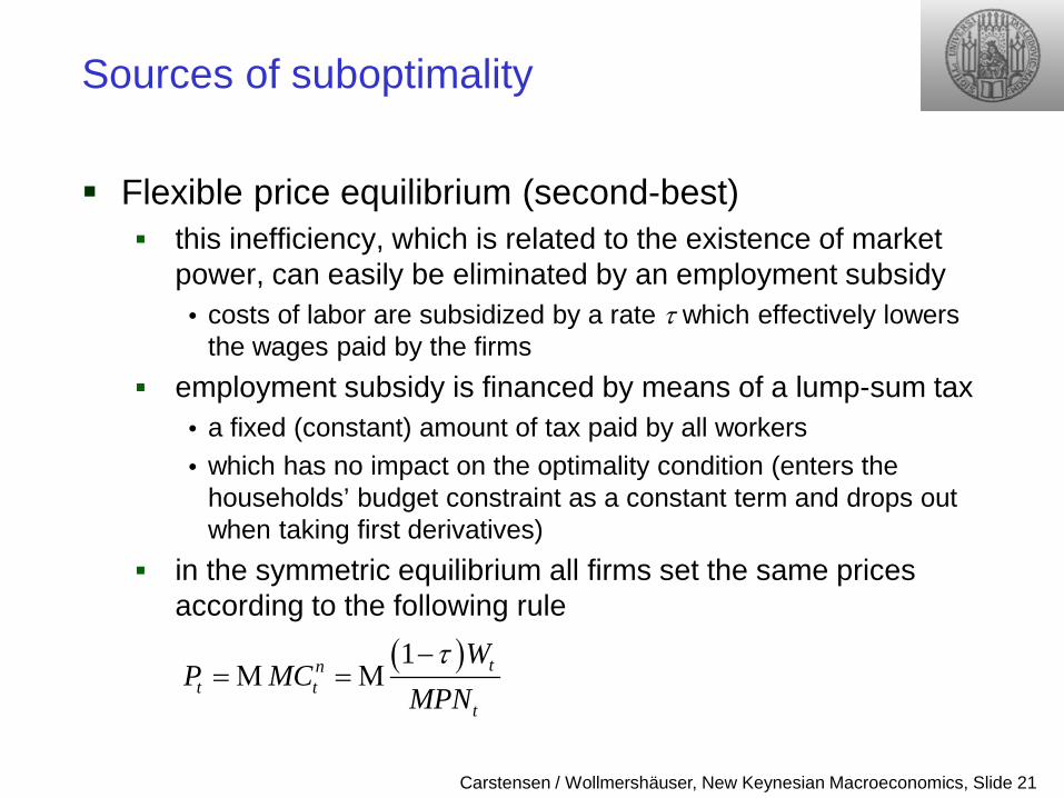
Flexible price equilibrium (second-best) this inefficiency, which is related to the existence of market
power, can easily be eliminated by an employment subsidy • costs of labor are subsidized by a rate τ which effectively lowers
the wages paid by the firms employment subsidy is financed by means of a lump-sum tax
• a fixed (constant) amount of tax paid by all workers • which has no impact on the optimality condition (enters the
households’ budget constraint as a constant term and drops out when taking first derivatives)
in the symmetric equilibrium all firms set the same prices according to the following rule
( )1 tnt t
t
WP MC
MPNτ−
= Μ = Μ
Carstensen / Wollmershäuser, New Keynesian Macroeconomics, Slide 22
Sources of suboptimality
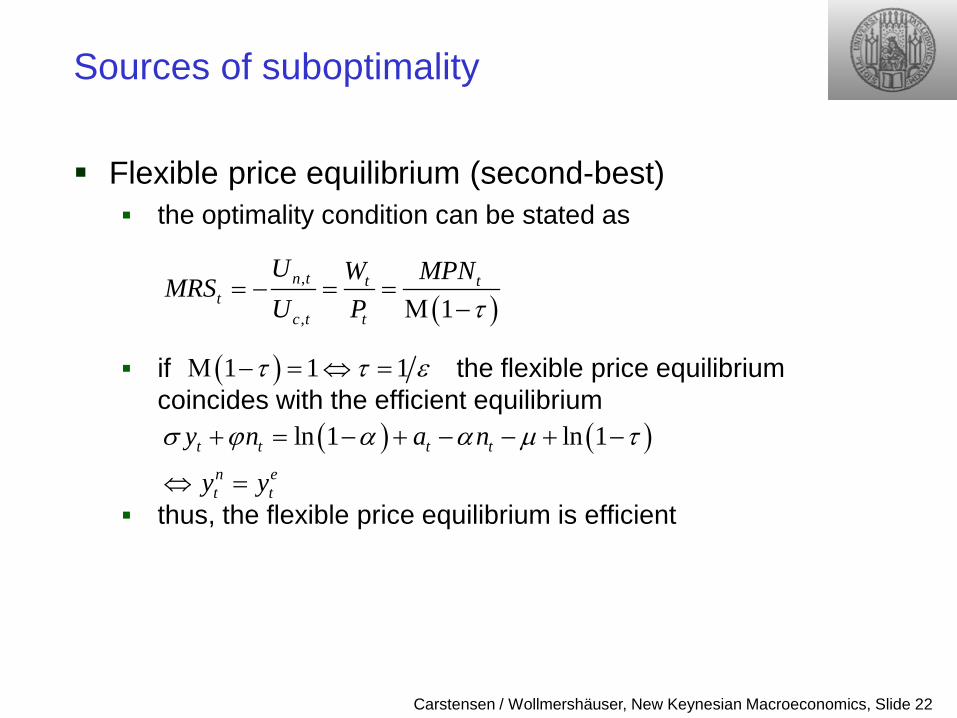
Flexible price equilibrium (second-best) the optimality condition can be stated as
if the flexible price equilibrium coincides with the efficient equilibrium
thus, the flexible price equilibrium is efficient
( ),
, 1n t t t
tc t t
U W MPNMRS
U P τ= − = =
Μ −
( )1 1 1τ τ εΜ − = ⇔ =
( ) ( )ln 1 ln 1t t t t
n et t
y n a n
y y
σ ϕ α α µ τ+ = − + − − + −
⇔ =
Carstensen / Wollmershäuser, New Keynesian Macroeconomics, Slide 23
Sources of suboptimality
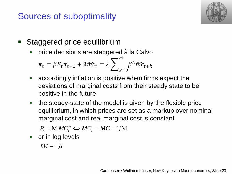
Staggered price equilibrium price decisions are staggered à la Calvo
𝜋𝑡 = 𝛽𝐸𝑡𝜋𝑡+1 + 𝜆𝑚𝑚𝑡 = 𝜆 𝛽𝑘𝑚𝑚𝑡+𝑘∞
𝑘=0
accordingly inflation is positive when firms expect the deviations of marginal costs from their steady state to be positive in the future
the steady-state of the model is given by the flexible price equilibrium, in which prices are set as a markup over nominal marginal cost and real marginal cost is constant
or in log levels 1n
t t tP MC MC MC= Μ ⇔ = = Μ
mc µ= −
Carstensen / Wollmershäuser, New Keynesian Macroeconomics, Slide 24
Sources of suboptimality
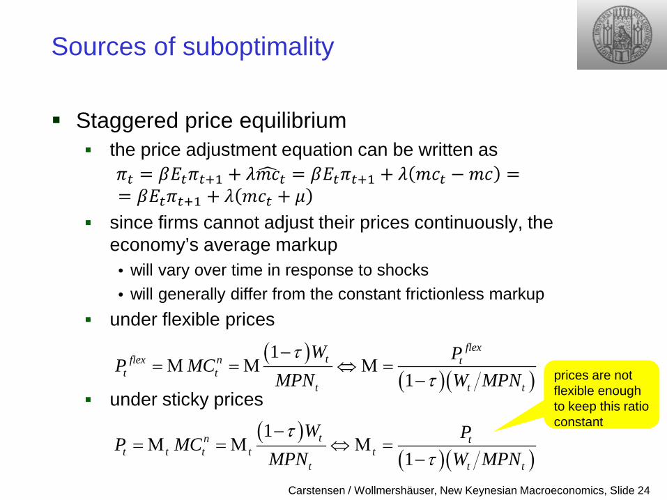
Staggered price equilibrium the price adjustment equation can be written as
𝜋𝑡 = 𝛽𝐸𝑡𝜋𝑡+1 + 𝜆𝑚𝑚𝑡 = 𝛽𝐸𝑡𝜋𝑡+1 + 𝜆 𝑚𝑚𝑡 − 𝑚𝑚 == 𝛽𝐸𝑡𝜋𝑡+1 + 𝜆 𝑚𝑚𝑡 + 𝜇
since firms cannot adjust their prices continuously, the economy’s average markup • will vary over time in response to shocks • will generally differ from the constant frictionless markup
under flexible prices
under sticky prices
( )( )( )
11
flextflex n t
t tt t t
W PP MC
MPN W MPNτ
τ−
= Μ = Μ ⇔Μ =−
( )( )( )
11
tn tt t t t t
t t t
W PP MC
MPN W MPNτ
τ−
= Μ = Μ ⇔Μ =−
prices are not flexible enough to keep this ratio constant
Carstensen / Wollmershäuser, New Keynesian Macroeconomics, Slide 25
Sources of suboptimality
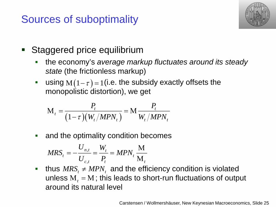
Staggered price equilibrium the economy’s average markup fluctuates around its steady
state (the frictionless markup) using (i.e. the subsidy exactly offsets the
monopolistic distortion), we get
and the optimality condition becomes
thus and the efficiency condition is violated unless ; this leads to short-run fluctuations of output around its natural level
( )( )1t t
tt t t t
P PW MPN W MPNτ
Μ = = Μ−
( )1 1τΜ − =
,
,
n t tt t
c t t t
U WMRS MPN
U PΜ
= − = =Μ
t tMRS MPN≠tΜ =Μ
Carstensen / Wollmershäuser, New Keynesian Macroeconomics, Slide 26
Sources of suboptimality
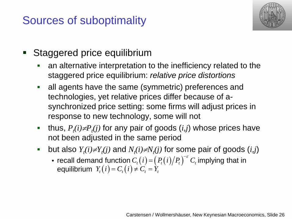
Staggered price equilibrium an alternative interpretation to the inefficiency related to the
staggered price equilibrium: relative price distortions all agents have the same (symmetric) preferences and
technologies, yet relative prices differ because of a-synchronized price setting: some firms will adjust prices in response to new technology, some will not
thus, Pt(i)≠Pt(j) for any pair of goods (i,j) whose prices have not been adjusted in the same period
but also Yt(i)≠Yt(j) and Nt(i)≠Nt(j) for some pair of goods (i,j) • recall demand function implying that in
equilibrium ( ) ( )( )t t t tC i P i P C
ε−=
( ) ( )t t t tY i C i C Y= ≠ =
Carstensen / Wollmershäuser, New Keynesian Macroeconomics, Slide 27
Optimal monetary policy I
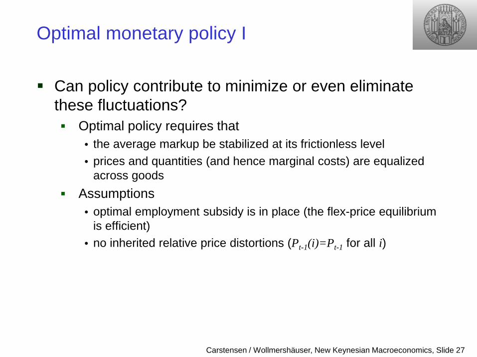
Can policy contribute to minimize or even eliminate these fluctuations? Optimal policy requires that
• the average markup be stabilized at its frictionless level • prices and quantities (and hence marginal costs) are equalized
across goods Assumptions
• optimal employment subsidy is in place (the flex-price equilibrium is efficient)
• no inherited relative price distortions (Pt-1(i)=Pt-1 for all i)
Carstensen / Wollmershäuser, New Keynesian Macroeconomics, Slide 28
Optimal monetary policy I
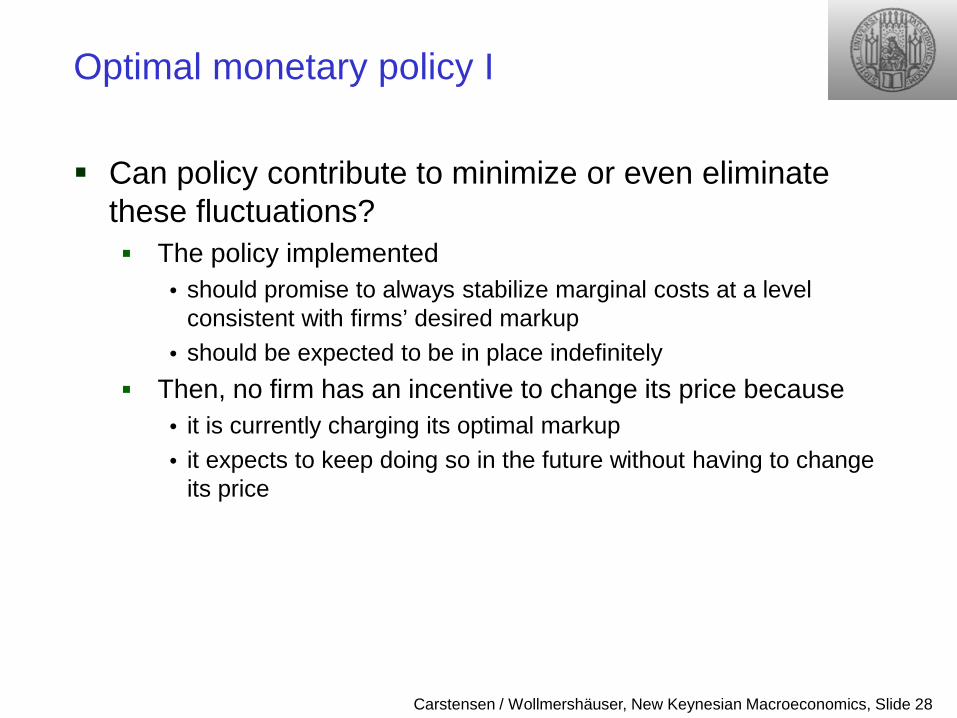
Can policy contribute to minimize or even eliminate these fluctuations? The policy implemented
• should promise to always stabilize marginal costs at a level consistent with firms’ desired markup
• should be expected to be in place indefinitely Then, no firm has an incentive to change its price because
• it is currently charging its optimal markup • it expects to keep doing so in the future without having to change
its price
Carstensen / Wollmershäuser, New Keynesian Macroeconomics, Slide 29
Optimal monetary policy I
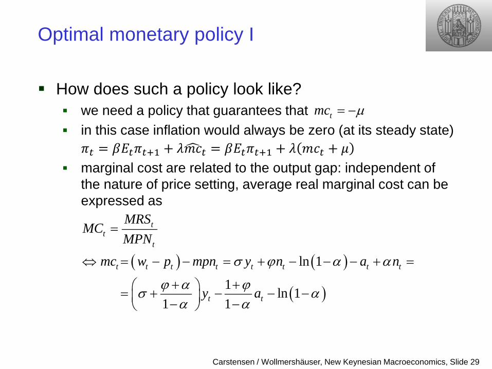
How does such a policy look like? we need a policy that guarantees that in this case inflation would always be zero (at its steady state)
𝜋𝑡 = 𝛽𝐸𝑡𝜋𝑡+1 + 𝜆𝑚𝑚𝑡 = 𝛽𝐸𝑡𝜋𝑡+1 + 𝜆 𝑚𝑚𝑡 + 𝜇 marginal cost are related to the output gap: independent of
the nature of price setting, average real marginal cost can be expressed as
tmc µ= −
( ) ( )
( )
ln 1
1 ln 11 1
tt
t
t t t t t t t t
t t
MRSMC
MPNmc w p mpn y n a n
y a
σ ϕ α α
ϕ α ϕσ αα α
=
⇔ = − − = + − − − + =
+ + = + − − − − −
Carstensen / Wollmershäuser, New Keynesian Macroeconomics, Slide 30
Optimal monetary policy I
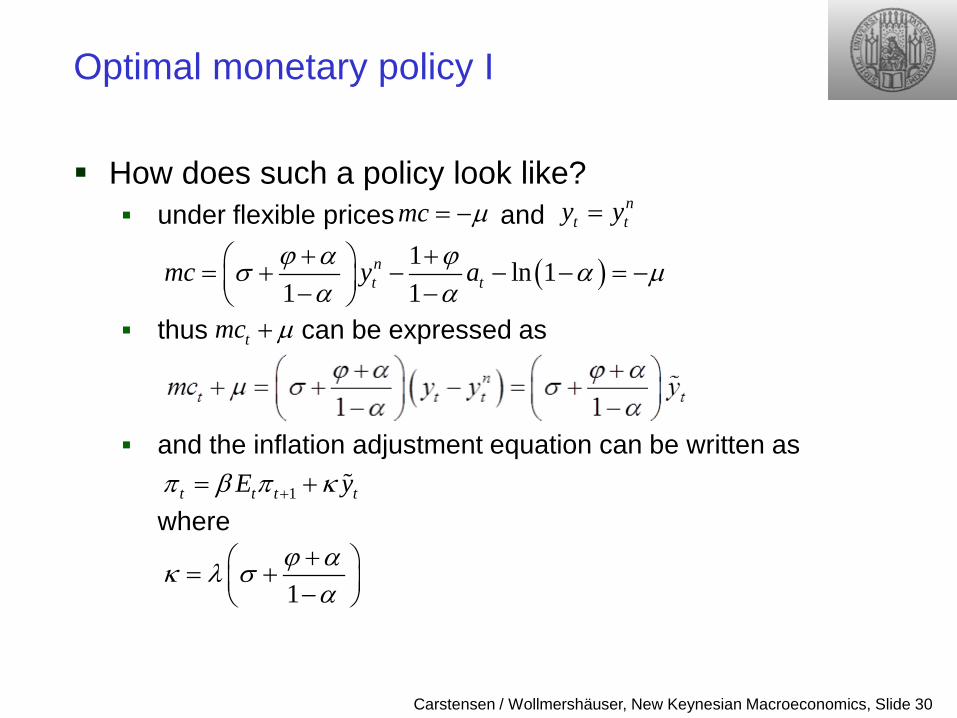
How does such a policy look like? under flexible prices and
thus can be expressed as
and the inflation adjustment equation can be written as
where
mc µ= − nt ty y=
( )1 ln 11 1
nt tmc y aϕ α ϕσ α µ
α α+ + = + − − − = − − −
tmc µ+
1π β π κ+= + t t t tE y
1ϕ ακ λ σ
α+ = + −
Carstensen / Wollmershäuser, New Keynesian Macroeconomics, Slide 31
Optimal monetary policy I
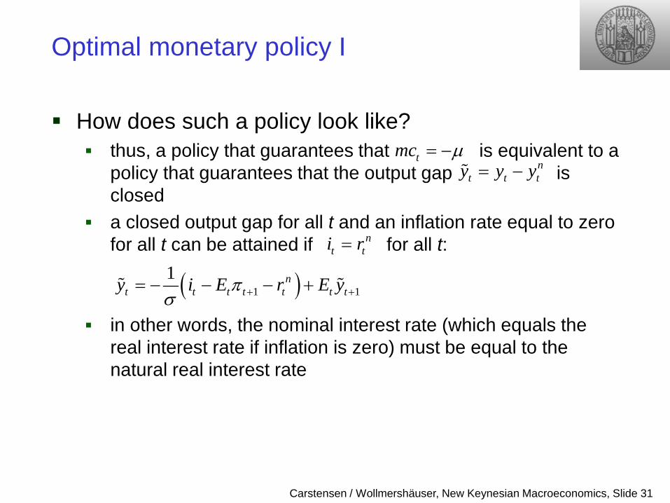
How does such a policy look like? thus, a policy that guarantees that is equivalent to a
policy that guarantees that the output gap is closed
a closed output gap for all t and an inflation rate equal to zero for all t can be attained if for all t:
in other words, the nominal interest rate (which equals the real interest rate if inflation is zero) must be equal to the natural real interest rate
tmc µ= −= − n
t t ty y y
( )1 11 πσ + += − − − + n
t t t t t t ty i E r E y
nt ti r=
Carstensen / Wollmershäuser, New Keynesian Macroeconomics, Slide 32
Optimal monetary policy I
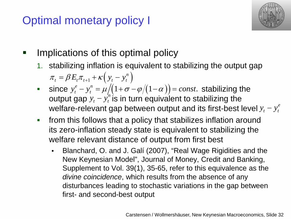
Implications of this optimal policy 1. stabilizing inflation is equivalent to stabilizing the output gap
since stabilizing the
output gap is in turn equivalent to stabilizing the welfare-relevant gap between output and its first-best level
from this follows that a policy that stabilizes inflation around its zero-inflation steady state is equivalent to stabilizing the welfare relevant distance of output from first best • Blanchard, O. and J. Galí (2007), “Real Wage Rigidities and the
New Keynesian Model”, Journal of Money, Credit and Banking, Supplement to Vol. 39(1), 35-65, refer to this equivalence as the divine coincidence, which results from the absence of any disturbances leading to stochastic variations in the gap between first- and second-best output
( )1n
t t t t tE y yπ β π κ+= + −
( )( )1 1 .e nt ty y constµ σ ϕ α− = + − − =
nt ty y−
et ty y−
Carstensen / Wollmershäuser, New Keynesian Macroeconomics, Slide 33
Optimal monetary policy I
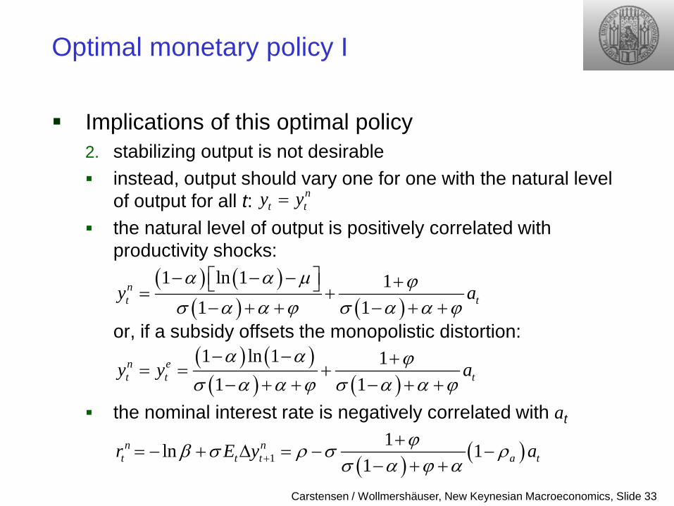
Implications of this optimal policy 2. stabilizing output is not desirable instead, output should vary one for one with the natural level
of output for all t: the natural level of output is positively correlated with
productivity shocks:
or, if a subsidy offsets the monopolistic distortion: the nominal interest rate is negatively correlated with at
nt ty y=
( ) ( )( ) ( )
1 ln 1 11 1
nt ty a
α α µ ϕσ α α ϕ σ α α ϕ
− − − + = +− + + − + +
( ) ( )( ) ( )
1 ln 1 11 1
n et t ty y a
α α ϕσ α α ϕ σ α α ϕ− − +
= = +− + + − + +
( ) ( )11ln 1
1n n
t t t a tr E y aϕβ σ ρ σ ρσ α ϕ α+
+= − + ∆ = − −
− + +
Carstensen / Wollmershäuser, New Keynesian Macroeconomics, Slide 34
Optimal monetary policy I
Implications of this optimal policy 3. price stability is a feature of optimal policy, even though the
policymaker does not attach any weight to such an objective price stability rather is a consequence of the efficient
allocation when prices are sticky the central bank’s objective is to make
all firms content with their existing prices • the assumed constraints on the adjustment of those prices are
effectively nonbinding • distortions due to relative price dispersion are eliminated (i.e.
Pt(i)/Pt(j)=1) price stability follows as a consequence of no firm willing to
adjust its price
Carstensen / Wollmershäuser, New Keynesian Macroeconomics, Slide 35
Optimal interest rate rules
Targeting the natural rate of interest the central bank adjusts the nominal interest rate one for one
with the natural real interest rate: • the nominal interest rate is a function of purely exogenous state
variables such a policy is able to produce the efficient allocation: however, the solution of the dynamical system associated
with this rule is not unique • in addition to the efficient allocation, a multiplicity of other
equilibria exist • it cannot be guaranteed that the efficient allocation will be the one
that will emerge in equilibrium • interpretation: lack of a nominal anchor
nt ti r=
0t ty tπ= = ∀
Carstensen / Wollmershäuser, New Keynesian Macroeconomics, Slide 36
Optimal interest rate rules
Targeting the natural rate of interest some remarks about determinacy
• cashless economy in which money plays no role – neither as a means of transaction – nor can the stock of money be used to determine the price
level • if it is not money that determines the price level, something else
must be in the model • in a neo-Wicksellian framework the fundamental determinants of
the price level are – the real factors that determine the equilibrium real rate of
interest – and the systematic relation between interest rates and prices
established by the central bank’s policy rule
Carstensen / Wollmershäuser, New Keynesian Macroeconomics, Slide 37
Optimal interest rate rules
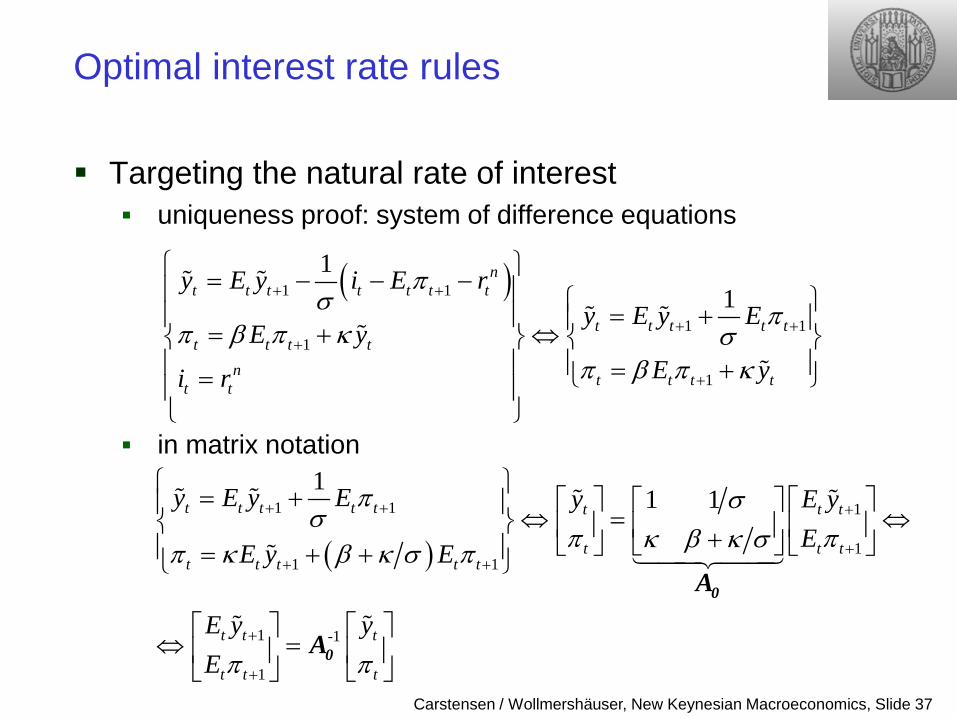
Targeting the natural rate of interest uniqueness proof: system of difference equations
in matrix notation
( )1 1
1 11
1
11
nt t t t t t t
t t t t tt t t t
n t t t tt t
y E y i E ry E y E
E yE yi r
πσ π
π β π κ σπ β π κ
+ +
+ ++
+
= − − − = + = + ⇔ = + =
( )1 1 1
11 1
1 -1
1
11 1t t t t t t t t
t t tt t t t t
t t t
t t t
y E y E y E yEE y E
E y yE
π σσ
π πκ β κ σπ κ β κ σ π
π π
+ + +
++ +
+
+
= + ⇔ = ⇔ + = + +
⇔ =
0
0
A
A
Carstensen / Wollmershäuser, New Keynesian Macroeconomics, Slide 38
Optimal interest rate rules
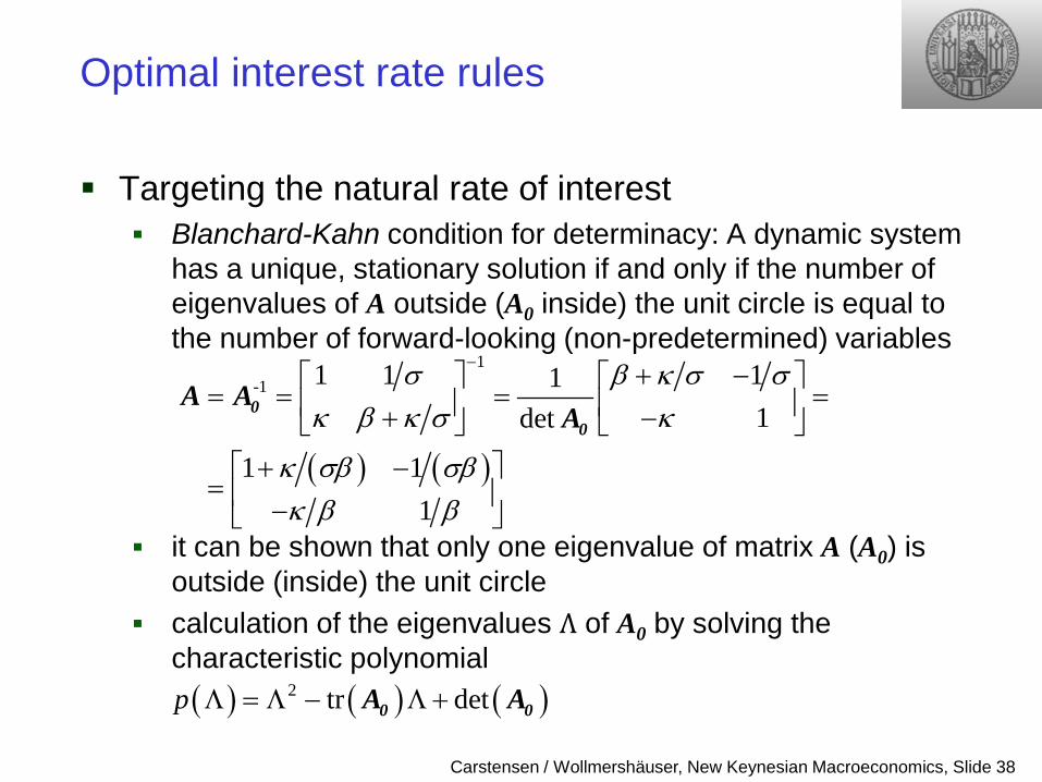
Targeting the natural rate of interest Blanchard-Kahn condition for determinacy: A dynamic system
has a unique, stationary solution if and only if the number of eigenvalues of A outside (A0 inside) the unit circle is equal to the number of forward-looking (non-predetermined) variables
it can be shown that only one eigenvalue of matrix A (A0) is outside (inside) the unit circle
calculation of the eigenvalues Λ of A0 by solving the characteristic polynomial
( ) ( )
1-1 1 1 11
1det
1 11
σ β κ σ σκ β κ σ κ
κ σβ σβκ β β
− + − = = = = + − + −
= −
00
A AA
( ) ( ) ( )2 tr detp Λ = Λ − Λ +0 0A A
Carstensen / Wollmershäuser, New Keynesian Macroeconomics, Slide 39
Optimal interest rate rules
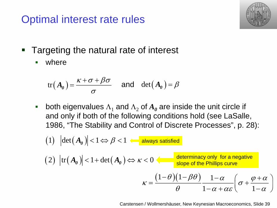
Targeting the natural rate of interest where
and
both eigenvalues Λ1 and Λ2 of A0 are inside the unit circle if
and only if both of the following conditions hold (see LaSalle, 1986, “The Stability and Control of Discrete Processes”, p. 28):
( )tr κ σ βσσ
+ +=0A ( )det β=0A
( ) ( )1 det 1 1β< ⇔ <0A
( ) ( ) ( )2 tr 1 det 0κ< + ⇔ <0 0A A
always satisfied
determinacy only for a negative slope of the Phillips curve
( )( )1 1 11 1
θ βθ α ϕ ακ σθ α αε α
− − − + = + − + −
Carstensen / Wollmershäuser, New Keynesian Macroeconomics, Slide 40
Optimal interest rate rules
Targeting the natural rate of interest if the equilibrium is indeterminate, then
• then an infinite number of different possible equilibrium responses of the endogenous variables to real disturbances exist
• some of these equilibria will lead to fluctuations in inflation and output which are disproportionately large relative to the size of the change in the “fundamentals” (technology shock) that has occurred
• some of these equilibria will lead to fluctuations in inflation and output in response to random events with no fundamental significance whatsoever
Lubik, T. A., and F. Schorfheide (2003), “Computing Sunspot Equilibria in Linear Rational Expectations Models”, in: Journal of Economic Dynamics and Control, Vol. 28(2), 273-285.
Carstensen / Wollmershäuser, New Keynesian Macroeconomics, Slide 41
Optimal interest rate rules
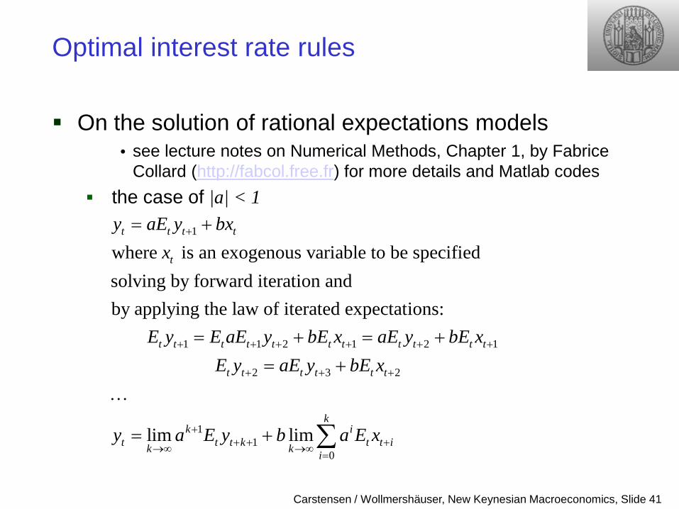
On the solution of rational expectations models • see lecture notes on Numerical Methods, Chapter 1, by Fabrice
Collard (http://fabcol.free.fr) for more details and Matlab codes the case of |a| < 1
1
1 1 2 1 2 1
2 3
where is an exogenous variable to be specifiedsolving by forward iteration and by applying the law of iterated expectations:
t t t t
t
t t t t t t t t t t t
t t t t
y aE y bxx
E y E aE y bE x aE y bE xE y aE y bE
+
+ + + + + +
+ +
= +
= + = +
= + 2
11
0lim lim
t t
kk i
t t t k t t ik k i
x
y a E y b a E x
+
++ + +→∞ →∞
=
= + ∑
Carstensen / Wollmershäuser, New Keynesian Macroeconomics, Slide 42
Optimal interest rate rules
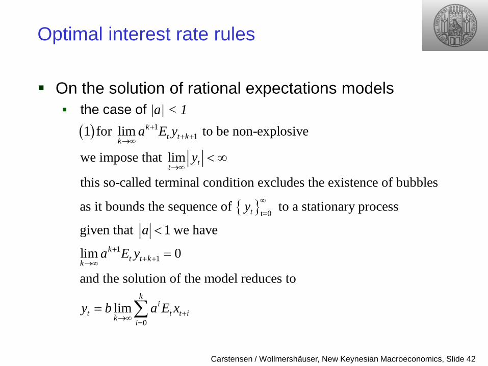
On the solution of rational expectations models the case of |a| < 1
( )
11
t=0
1 for lim to be non-explosive
we impose that lim
this so-called terminal condition excludes the existence of bubbles
as it bounds the sequence of to a stationary process
given
kt t kk
tt
t
a E y
y
y
++ +→∞
→∞
∞
< ∞
11
0
that 1 we have
lim 0
and the solution of the model reduces to
lim
kt t kk
ki
t t t ik i
a
a E y
y b a E x
++ +→∞
+→∞=
<
=
= ∑
Carstensen / Wollmershäuser, New Keynesian Macroeconomics, Slide 43
Optimal interest rate rules
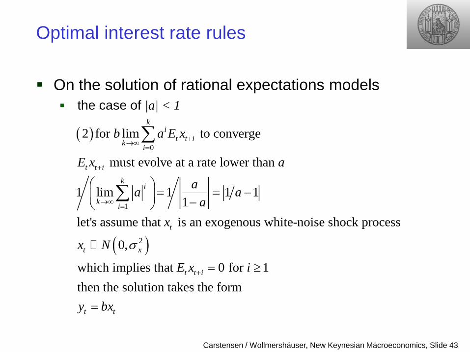
On the solution of rational expectations models the case of |a| < 1
( )
( )
0
1
2
2 for lim to converge
must evolve at a rate lower than
1 lim 1 1 11
let's assume that is an exogenous white-noise shock process
0,
which implies that
ki
t t ik i
t t i
ki
k i
t
t x
b a E x
E x a
aa aa
x
x N
E
σ
+→∞=
+
→∞=
= = − −
∑
∑
0 for 1then the solution takes the form
t t i
t t
x i
y bx
+ = ≥
=
Carstensen / Wollmershäuser, New Keynesian Macroeconomics, Slide 44
Optimal interest rate rules
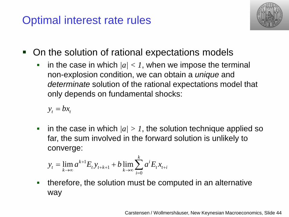
On the solution of rational expectations models in the case in which |a| < 1, when we impose the terminal
non-explosion condition, we can obtain a unique and determinate solution of the rational expectations model that only depends on fundamental shocks:
in the case in which |a| > 1, the solution technique applied so far, the sum involved in the forward solution is unlikely to converge:
therefore, the solution must be computed in an alternative way
11
0lim lim
kk i
t t t k t t ik k iy a E y b a E x+
+ + +→∞ →∞=
= + ∑
t ty bx=
Carstensen / Wollmershäuser, New Keynesian Macroeconomics, Slide 45
Optimal interest rate rules
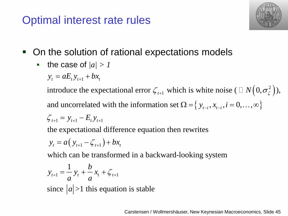
On the solution of rational expectations models the case of |a| > 1
( )
1
21
1 1 1
introduce the expectational error which is white noise ( 0, ),
and uncorrelated with the information set , , 0, ,
the expectational difference equation
t t t t
t
t i t i
t t t t
y aE y bx
N
y x iy E y
ζζ σ
ζ
+
+
− −
+ + +
= +
Ω = = ∞
= −
( )1 1
1 1
then rewrites which can be transformed in a backward-looking system
1
since >1 this equation is stable
t t t t
t t t t
y a y bx
by y xa aa
ζ
ζ
+ +
+ +
= − +
= + +
Carstensen / Wollmershäuser, New Keynesian Macroeconomics, Slide 46
Optimal interest rate rules
On the solution of rational expectations models the case of |a| > 1
1 1
0
1
the problem with this equation is, however, that for a given realization of the fundamental shock there is an infinite number
of solutions for the process
WHY?because there
t t t t
t
t t
by y xa a
x
y
ζ+ +
∞
=
= + +
is an infinite number of specifications of the processfor the expectational error
Carstensen / Wollmershäuser, New Keynesian Macroeconomics, Slide 47
Optimal interest rate rules
On the solution of rational expectations models in the case in which |a| > 1 we can obtain an infinite number
of solutions of the rational expectations model in this case the solution is said to be indeterminate note
• that these solutions are stable, implying that the economy always converges to its long-run solution
• that the dynamics of the economy depends on the volatility of the non-fundamental shock (the expectational error)
Carstensen / Wollmershäuser, New Keynesian Macroeconomics, Slide 48
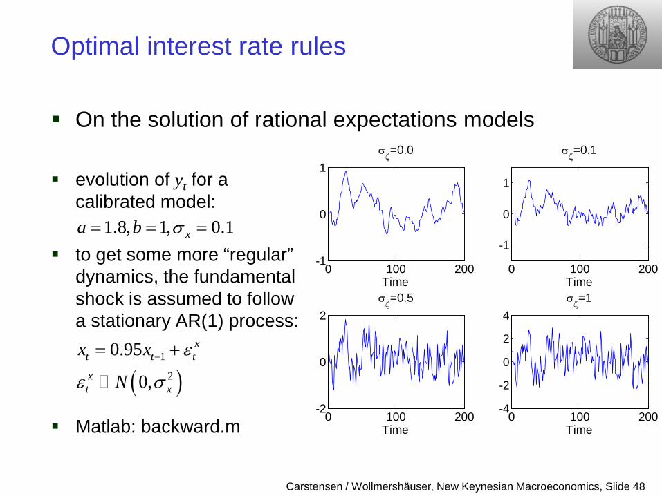
Optimal interest rate rules
evolution of yt for a calibrated model:
to get some more “regular” dynamics, the fundamental shock is assumed to follow a stationary AR(1) process:
Matlab: backward.m
0 100 200-1
0
1
Time
σζ=0.0
0 100 200
-1
0
1
Time
σζ=0.1
0 100 200-2
0
2
Time
σζ=0.5
0 100 200-4
-2
0
2
4
Time
σζ=1
On the solution of rational expectations models
1.8, 1, 0.1xa b σ= = =
( )1
2
0.95
0,
xt t t
xt x
x x
N
ε
ε σ−= +
Carstensen / Wollmershäuser, New Keynesian Macroeconomics, Slide 49
Optimal interest rate rules
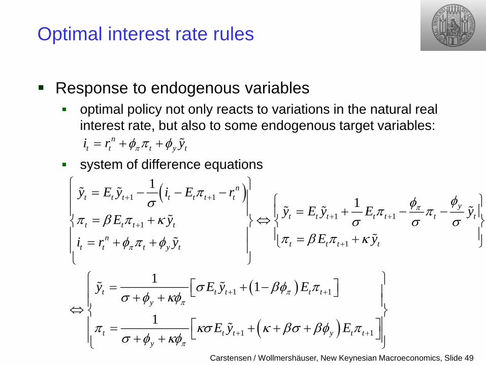
Response to endogenous variables optimal policy not only reacts to variations in the natural real
interest rate, but also to some endogenous target variables:
system of difference equations
nt t t y ti r yπφ π φ= + +
( )
( )
( )
1 1
1 11
1
1 1
1
11
1 1
1
nt t t t t t t
yt t t t t t t
t t t tn
t t t tt t t y t
t t t t ty
t t t yy
y E y i E ry E y E yE y
E yi r y
y E y E
E y
π
π
ππ
π
π φφσ π ππ β π κ σ σ σπ β π κφ π φ
σ βφ πσ φ κφ
π κσ κ βσ βφσ φ κφ
+ +
+ ++
+
+ +
+
= − − − = + − − = + ⇔ = += + +
= + − + +⇔
= + + ++ +
1t tE π +
Carstensen / Wollmershäuser, New Keynesian Macroeconomics, Slide 50
Optimal interest rate rules
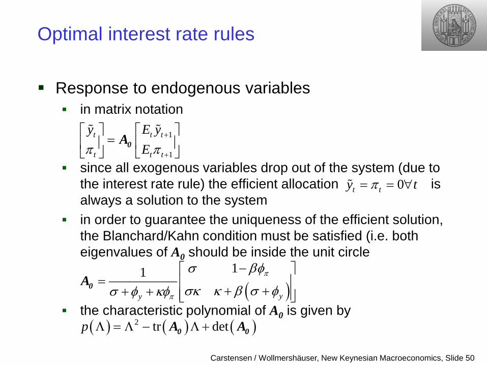
Response to endogenous variables in matrix notation
since all exogenous variables drop out of the system (due to the interest rate rule) the efficient allocation is always a solution to the system
in order to guarantee the uniqueness of the efficient solution, the Blanchard/Kahn condition must be satisfied (i.e. both eigenvalues of A0 should be inside the unit circle
the characteristic polynomial of A0 is given by
1
1
t t t
t t t
y E yEπ π
+
+
=
0A
0t ty tπ= = ∀
( )11
yy
π
π
σ βφ
σκ κ β σ φσ φ κφ
− =
+ ++ + 0A
( ) ( ) ( )2 tr detp Λ = Λ − Λ +0 0A A
Carstensen / Wollmershäuser, New Keynesian Macroeconomics, Slide 51
Optimal interest rate rules
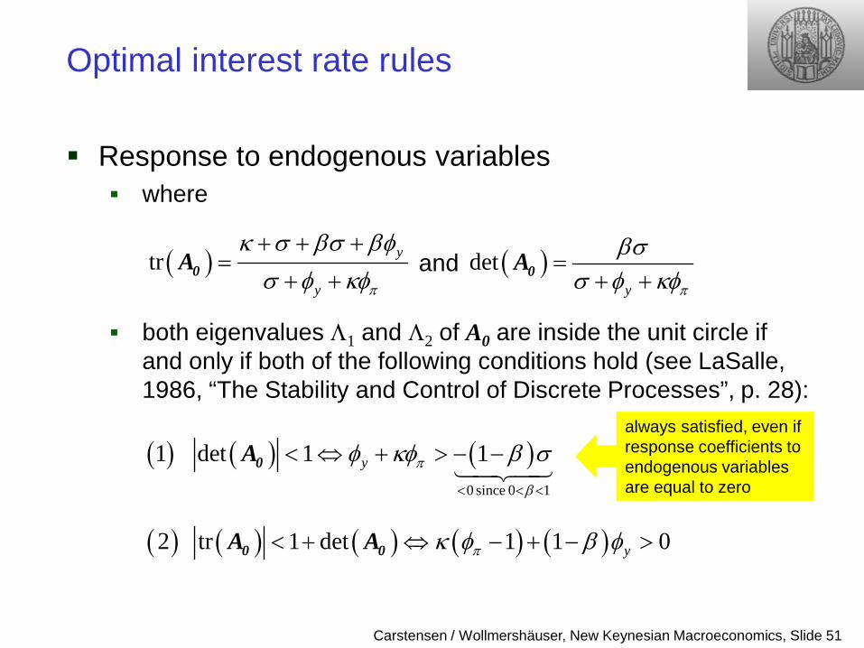
Response to endogenous variables where
and
both eigenvalues Λ1 and Λ2 of A0 are inside the unit circle if
and only if both of the following conditions hold (see LaSalle, 1986, “The Stability and Control of Discrete Processes”, p. 28):
( )tr y
y π
κ σ βσ βφσ φ κφ+ + +
=+ +0A ( )det
y π
βσσ φ κφ
=+ +0A
( ) ( ) ( )0 since 0 1
1 det 1 1y π
β
φ κφ β σ< < <
< ⇔ + > − −0A
( ) ( ) ( ) ( ) ( )2 tr 1 det 1 1 0yπκ φ β φ< + ⇔ − + − >0 0A A
always satisfied, even if response coefficients to endogenous variables are equal to zero
Carstensen / Wollmershäuser, New Keynesian Macroeconomics, Slide 52
Optimal interest rate rules
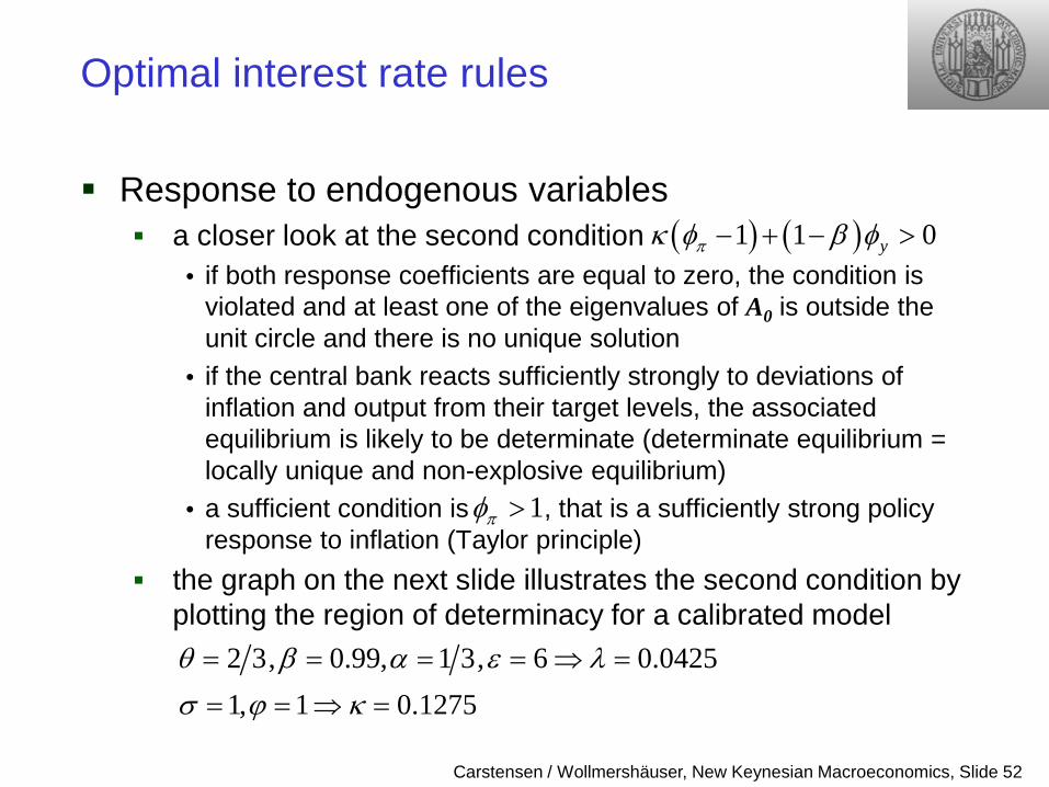
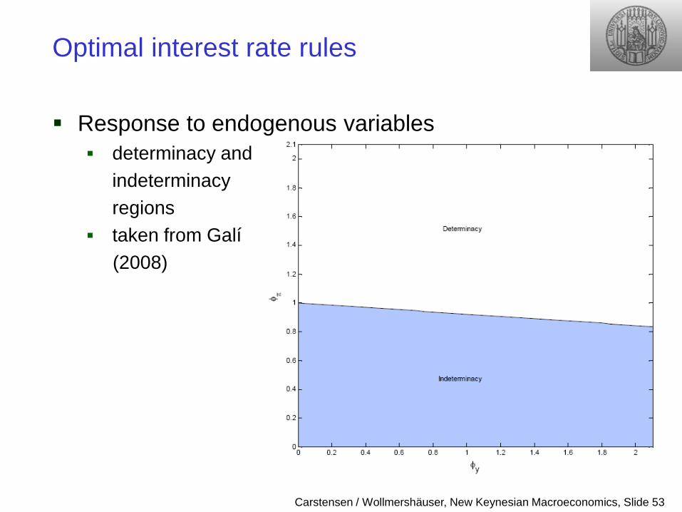
Response to endogenous variables a closer look at the second condition
• if both response coefficients are equal to zero, the condition is violated and at least one of the eigenvalues of A0 is outside the unit circle and there is no unique solution
• if the central bank reacts sufficiently strongly to deviations of inflation and output from their target levels, the associated equilibrium is likely to be determinate (determinate equilibrium = locally unique and non-explosive equilibrium)
• a sufficient condition is , that is a sufficiently strong policy response to inflation (Taylor principle)
the graph on the next slide illustrates the second condition by plotting the region of determinacy for a calibrated model
( ) ( )1 1 0yπκ φ β φ− + − >
1, 1 0.1275σ ϕ κ= = ⇒ =
2 3, 0.99, 1 3, 6 0.0425θ β α ε λ= = = = ⇒ =
1πφ >
Carstensen / Wollmershäuser, New Keynesian Macroeconomics, Slide 53
Optimal interest rate rules
Response to endogenous variables determinacy and indeterminacy regions taken from Galí
(2008)
Carstensen / Wollmershäuser, New Keynesian Macroeconomics, Slide 54
Optimal interest rate rules
Response to endogenous variables the unique equilibrium involves from this follows that the interest rate rule effectively
collapses to thus the existence of a credible policy threat to react
sufficiently strongly to inflation-output gap developments is sufficient to prevent any movements in these variables!
moreover, such a rule provides the cashless economy with a nominal anchor that determines the equilibrium path of interest rates and prices
0t ty tπ= = ∀
nt ti r t= ∀
Carstensen / Wollmershäuser, New Keynesian Macroeconomics, Slide 55
Optimal interest rate rules
Response to endogenous variables a forward-looking policy rule
since all exogenous variables drop out of the system the
efficient allocation is always a solution to the system
for both eigenvalues of A0 to be within the unit circle the following two conditions must hold
1 1n
t t t t y t ti r E E yπφ π φ+ += + +
1
1
t t t
t t t
y E yEπ π
+
+
=
0A
( )1 1
1 1
1
1y
y
π
π
σ φ σ φ
κ σ φ β κσ φ
− −
− −
− − =
− − 0A
( ) ( )( ) ( ) ( )
1 1 0
1 1 2 1y
y
π
π
κ φ β φ
κ φ β φ σ β
− + − >
− + + < +
Carstensen / Wollmershäuser, New Keynesian Macroeconomics, Slide 56
Optimal interest rate rules
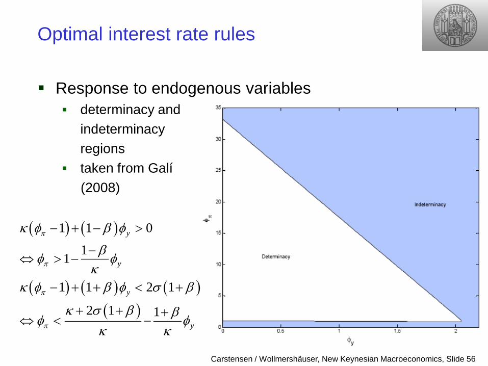
Response to endogenous variables determinacy and indeterminacy regions taken from Galí
(2008)
( ) ( )
( ) ( ) ( )( )
1 1 0
11
1 1 2 1
2 1 1
y
y
y
y
π
π
π
π
κ φ β φ
βφ φκ
κ φ β φ σ β
κ σ β βφ φκ κ
− + − >
−⇔ > −
− + + < +
+ + +⇔ < −
Carstensen / Wollmershäuser, New Keynesian Macroeconomics, Slide 57
Simple policy rules I
Optimal interest rate rules require that the exogenous state variables of the economy
are observable here
• the natural rate of interest • the natural level of output (to compute the output gap)
unrealistic, since it requires exact knowledge of the economy’s model, the parameter values, and the realized value of the shocks
Simple interest rate rules defined as interest rate rules that makes the policy instrument
a function of observable variables only do not require the above knowledge
Carstensen / Wollmershäuser, New Keynesian Macroeconomics, Slide 58
Simple policy rules I
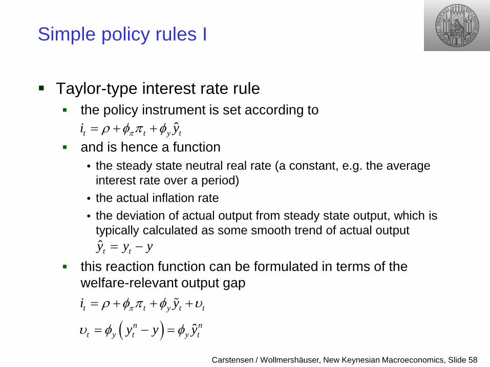
Taylor-type interest rate rule the policy instrument is set according to
and is hence a function
• the steady state neutral real rate (a constant, e.g. the average interest rate over a period)
• the actual inflation rate • the deviation of actual output from steady state output, which is
typically calculated as some smooth trend of actual output
this reaction function can be formulated in terms of the welfare-relevant output gap
ˆt t y ti yπρ φ π φ= + +
t t y t ti yπρ φ π φ υ= + + +
( ) ˆn nt y t y ty y yυ φ φ= − =
ˆt ty y y= −
Carstensen / Wollmershäuser, New Keynesian Macroeconomics, Slide 59
Simple policy rules I
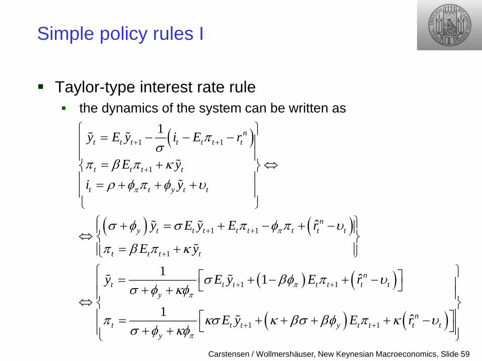
Taylor-type interest rate rule the dynamics of the system can be written as
( )
( ) ( )
( ) ( )
1 1
1
1 1
1
1 1
1
ˆ
1 ˆ1
1
nt t t t t t t
t t t t
t t y t t
ny t t t t t t t t
t t t t
nt t t t t t t
y
t ty
y E y i E r
E yi y
y E y E r
E y
y E y E r
E
π
π
ππ
π
πσ
π β π κρ φ π φ υ
σ φ σ π φ π υ
π β π κ
σ βφ π υσ φ κφ
π κσσ φ κφ
+ +
+
+ +
+
+ +
= − − −
= + ⇔ = + + +
+ = + − + − ⇔ = +
= + − + − + +⇔
=+ +
( ) ( )1 1 ˆnt y t t t ty E rκ βσ βφ π κ υ+ +
+ + + + −
Carstensen / Wollmershäuser, New Keynesian Macroeconomics, Slide 60
Simple policy rules I
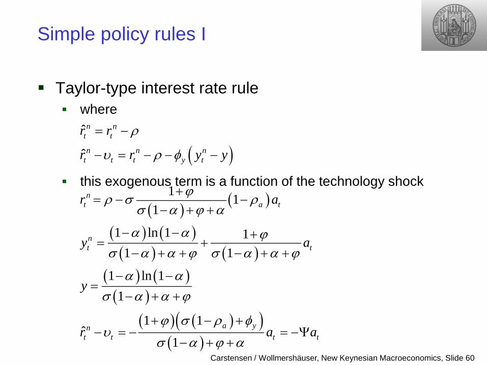
Taylor-type interest rate rule where
this exogenous term is a function of the technology shock
ˆn nt tr r ρ= −
( )ˆn n nt t t y tr r y yυ ρ φ− = − − −
( ) ( )
( ) ( )( ) ( )
( ) ( )( )
( ) ( )( )( )
1 11
1 ln 1 11 1
1 ln 11
1 1ˆ
1
nt a t
nt t
a ynt t t t
r a
y a
y
r a a
ϕρ σ ρσ α ϕ α
α α ϕσ α α ϕ σ α α ϕ
α ασ α α ϕ
ϕ σ ρ φυ
σ α ϕ α
+= − −
− + +
− − += +
− + + − + +
− −=
− + +
+ − +− = − = −Ψ
− + +
Carstensen / Wollmershäuser, New Keynesian Macroeconomics, Slide 61
Simple policy rules I
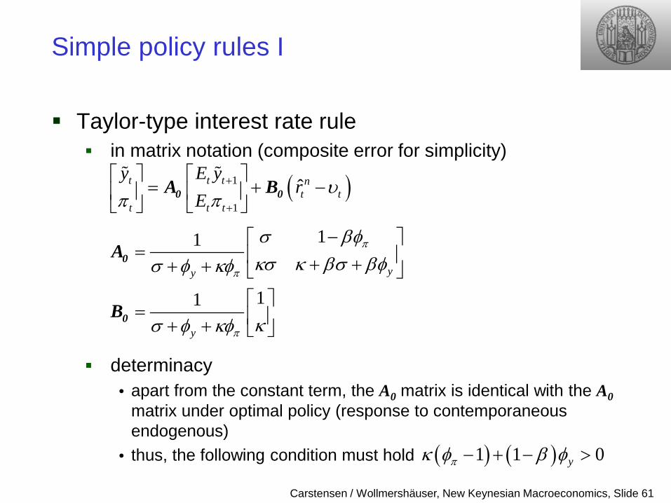
Taylor-type interest rate rule in matrix notation (composite error for simplicity)
determinacy • apart from the constant term, the A0 matrix is identical with the A0
matrix under optimal policy (response to contemporaneous endogenous)
• thus, the following condition must hold
( )1
1
ˆt t t nt t
t t t
y E yr
Eυ
π π+
+
= + −
0 0A B
11
11
yy
y
π
π
π
σ βφκσ κ βσ βφσ φ κφ
κσ φ κφ
− = + ++ +
= + +
0
0
A
B
( ) ( )1 1 0yπκ φ β φ− + − >
Carstensen / Wollmershäuser, New Keynesian Macroeconomics, Slide 62
Simple policy rules I
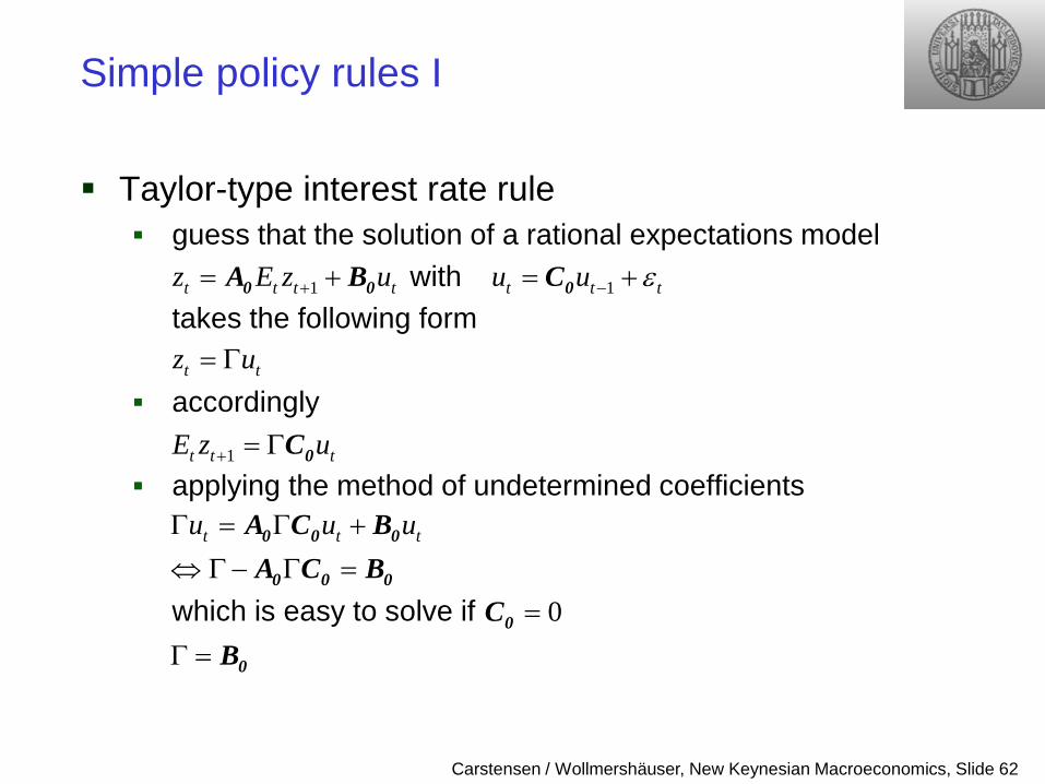
Taylor-type interest rate rule guess that the solution of a rational expectations model with takes the following form accordingly
applying the method of undetermined coefficients
which is easy to solve if
1t t t tz E z u+= +0 0A B
t tz u= Γ
1t t tE z u+ = Γ 0C
1t t tu u ε−= +0C
t t tu u uΓ = Γ +
⇔ Γ− Γ =0 0 0
0 0 0
A C BA C B
0=0CΓ = 0B
Carstensen / Wollmershäuser, New Keynesian Macroeconomics, Slide 63
Simple policy rules I
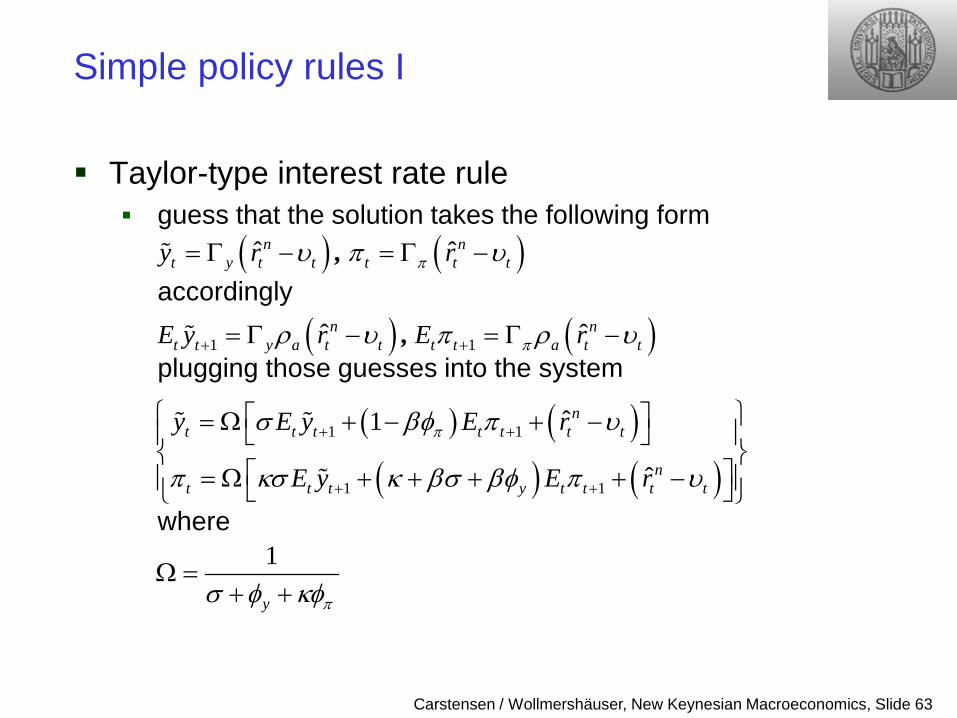
Taylor-type interest rate rule guess that the solution takes the following form
accordingly plugging those guesses into the system where
( ) ( )ˆ ˆn nt y t t t t ty r rπυ π υ= Γ − = Γ − ,
( ) ( )1 1ˆ ˆn nt t y a t t t t a t tE y r E rπρ υ π ρ υ+ += Γ − = Γ − ,
( ) ( )( ) ( )
1 1
1 1
ˆ1
ˆ
nt t t t t t t
nt t t y t t t t
y E y E r
E y E r
πσ βφ π υ
π κσ κ βσ βφ π υ
+ +
+ +
= Ω + − + −
= Ω + + + + −
1
y πσ φ κφΩ =
+ +
Carstensen / Wollmershäuser, New Keynesian Macroeconomics, Slide 64
Simple policy rules I
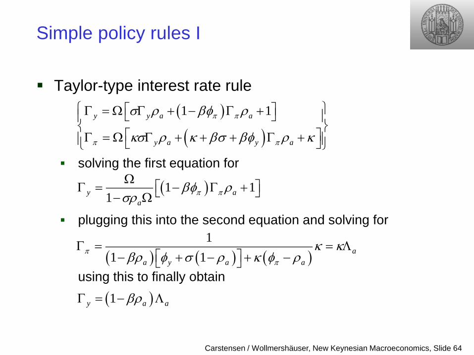
Taylor-type interest rate rule
solving the first equation for
plugging this into the second equation and solving for
using this to finally obtain
( )
( )1 1y y a a
y a y a
π π
π π
σ ρ βφ ρ
κσ ρ κ βσ βφ ρ κ
Γ = Ω Γ + − Γ +
Γ = Ω Γ + + + Γ +
( )1 11y a
aπ πβφ ρ
σρΩ
Γ = − Γ + − Ω
( ) ( ) ( )1
1 1 aa y a a
ππ
κ κβρ φ σ ρ κ φ ρ
Γ = = Λ − + − + −
( )1y a aβρΓ = − Λ
Carstensen / Wollmershäuser, New Keynesian Macroeconomics, Slide 65
Simple policy rules I
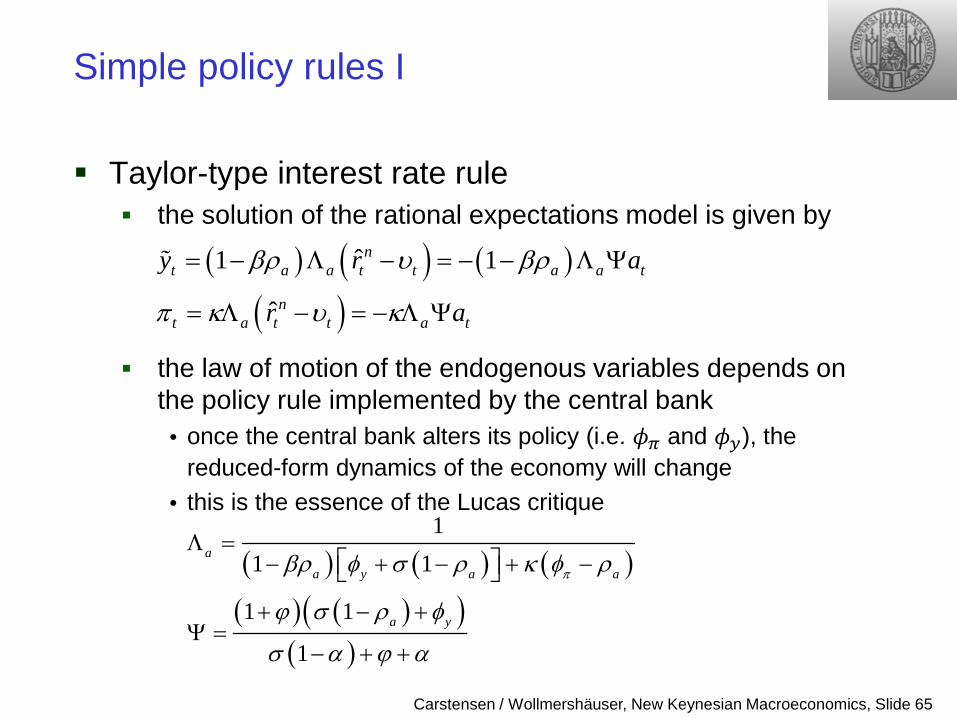
Taylor-type interest rate rule the solution of the rational expectations model is given by
the law of motion of the endogenous variables depends on the policy rule implemented by the central bank • once the central bank alters its policy (i.e. 𝜙𝜋 and 𝜙𝑦), the
reduced-form dynamics of the economy will change • this is the essence of the Lucas critique
( ) ( ) ( )
( )ˆ1 1
ˆ
nt a a t t a a t
nt a t t a t
y r a
r a
βρ υ βρ
π κ υ κ
= − Λ − = − − Λ Ψ
= Λ − = − Λ Ψ
( ) ( ) ( )( ) ( )( )
( )
11 1
1 1
1
aa y a a
a y
πβρ φ σ ρ κ φ ρ
ϕ σ ρ φ
σ α ϕ α
Λ =− + − + −
+ − +Ψ =
− + +
Carstensen / Wollmershäuser, New Keynesian Macroeconomics, Slide 66
Simple policy rules I
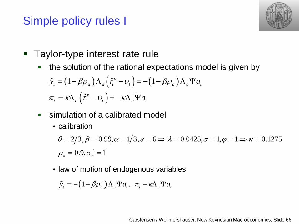
Taylor-type interest rate rule the solution of the rational expectations model is given by
simulation of a calibrated model • calibration
• law of motion of endogenous variables
( ) ( ) ( )
( )ˆ1 1
ˆ
nt a a t t a a t
nt a t t a t
y r a
r a
βρ υ βρ
π κ υ κ
= − Λ − = − − Λ Ψ
= Λ − = − Λ Ψ
2
2 3, 0.99, 1 3, 6 0.0425, 1, 1 0.1275
0.9, 1a ε
θ β α ε λ σ ϕ κ
ρ σ
= = = = ⇒ = = = ⇒ =
= =
( )1 ,t a a t t a ty a aβρ π κ= − − Λ Ψ − Λ Ψ
Carstensen / Wollmershäuser, New Keynesian Macroeconomics, Slide 67
Simple policy rules I
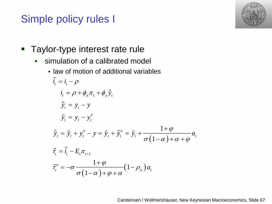
Taylor-type interest rate rule simulation of a calibrated model
• law of motion of additional variables
( )
( )( )
1
ˆ
ˆ
ˆ
1ˆ ˆ1
ˆˆ
1ˆ 11
t t
t t y t
t t
nt t t
n nt t t t t t t
t t t t
nt a t
i i
i y
y y y
y y y
y y y y y y y a
r i E
r a
π
ρ
ρ φ π φ
ϕσ α α ϕ
π
ϕσ ρσ α ϕ α
+
= −
= + +
= −
= −
+= + − = + = +
− + +
= −
+= − −
− + +
Carstensen / Wollmershäuser, New Keynesian Macroeconomics, Slide 68
Simple policy rules I
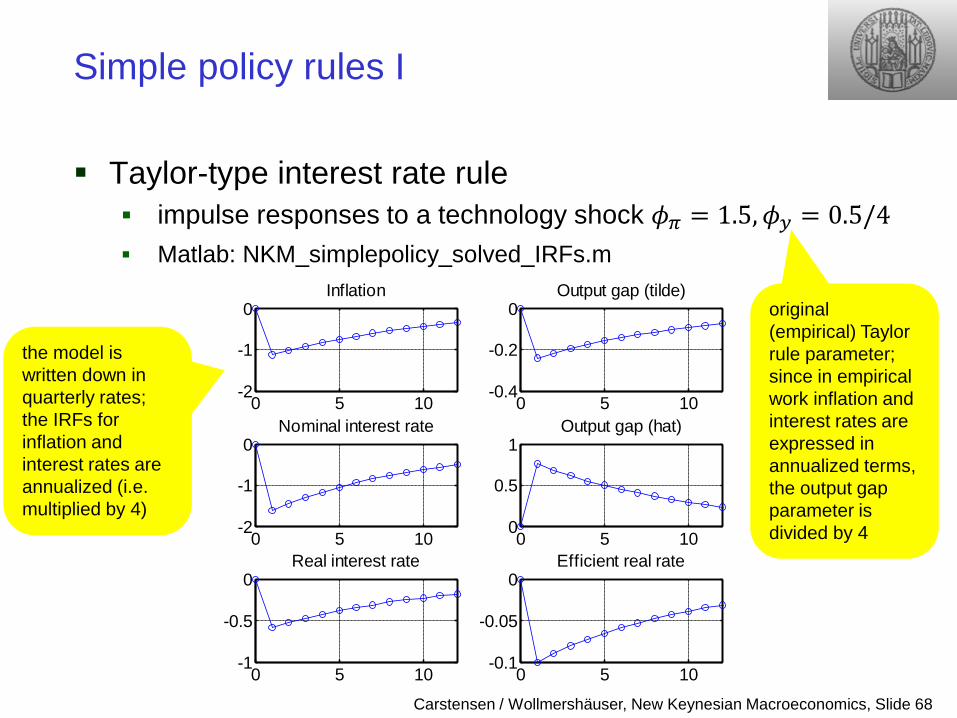
Taylor-type interest rate rule impulse responses to a technology shock 𝜙𝜋 = 1.5,𝜙𝑦 = 0.5/4 Matlab: NKM_simplepolicy_solved_IRFs.m
0 5 10-2
-1
0Inflation
0 5 10-0.4
-0.2
0Output gap (tilde)
0 5 10-2
-1
0Nominal interest rate
0 5 100
0.5
1Output gap (hat)
0 5 10-1
-0.5
0Real interest rate
0 5 10-0.1
-0.05
0Efficient real rate
the model is written down in quarterly rates; the IRFs for inflation and interest rates are annualized (i.e. multiplied by 4)
original (empirical) Taylor rule parameter; since in empirical work inflation and interest rates are expressed in annualized terms, the output gap parameter is divided by 4
Carstensen / Wollmershäuser, New Keynesian Macroeconomics, Slide 69
Simple policy rules I
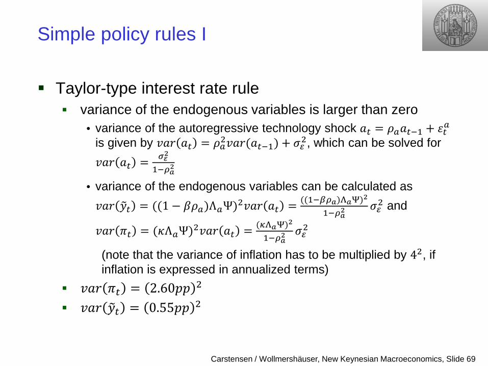
Taylor-type interest rate rule variance of the endogenous variables is larger than zero
• variance of the autoregressive technology shock 𝑎𝑡 = 𝜌𝑎𝑎𝑡−1 + 𝜀𝑡𝑎 is given by 𝑣𝑎𝑣 𝑎𝑡 = 𝜌𝑎2𝑣𝑎𝑣(𝑎𝑡−1) + 𝜎𝜀2, which can be solved for 𝑣𝑎𝑣 𝑎𝑡 = 𝜎𝜀2
1−𝜌𝑎2
• variance of the endogenous variables can be calculated as 𝑣𝑎𝑣 𝑦𝑡 = ((1 − 𝛽𝜌𝑎)Λ𝑎Ψ)2𝑣𝑎𝑣 𝑎𝑡 = ((1−𝛽𝜌𝑎)Λ𝑎Ψ)2
1−𝜌𝑎2𝜎𝜀2 and
𝑣𝑎𝑣 𝜋𝑡 = (𝜅Λ𝑎Ψ)2𝑣𝑎𝑣 𝑎𝑡 = (𝜅Λ𝑎Ψ)2
1−𝜌𝑎2𝜎𝜀2
(note that the variance of inflation has to be multiplied by 42, if inflation is expressed in annualized terms)
𝑣𝑎𝑣 𝜋𝑡 = 2.60𝑝𝑝 2 𝑣𝑎𝑣 𝑦𝑡 = 0.55𝑝𝑝 2
Carstensen / Wollmershäuser, New Keynesian Macroeconomics, Slide 70
Simple policy rules I
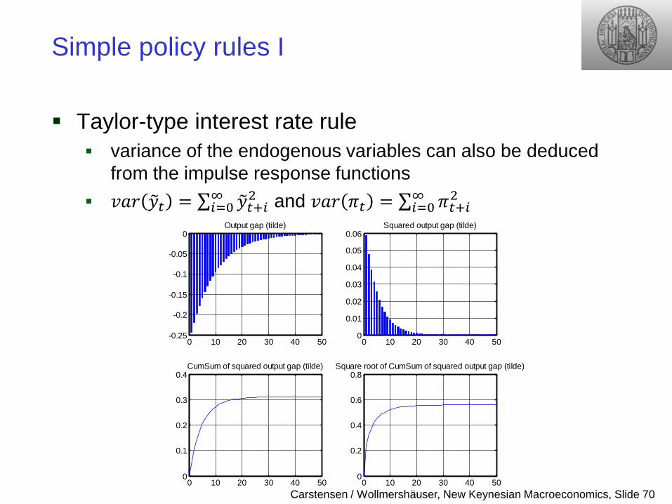
Taylor-type interest rate rule variance of the endogenous variables can also be deduced
from the impulse response functions 𝑣𝑎𝑣 𝑦𝑡 = ∑ 𝑦𝑡+𝑖2∞
𝑖=0 and 𝑣𝑎𝑣 𝜋𝑡 = ∑ 𝜋𝑡+𝑖2∞𝑖=0
0 10 20 30 40 50-0.25
-0.2
-0.15
-0.1
-0.05
0Output gap (tilde)
0 10 20 30 40 500
0.01
0.02
0.03
0.04
0.05
0.06Squared output gap (tilde)
0 10 20 30 40 500
0.1
0.2
0.3
0.4CumSum of squared output gap (tilde)
0 10 20 30 40 500
0.2
0.4
0.6
0.8Square root of CumSum of squared output gap (tilde)
Carstensen / Wollmershäuser, New Keynesian Macroeconomics, Slide 71
Simple policy rules I
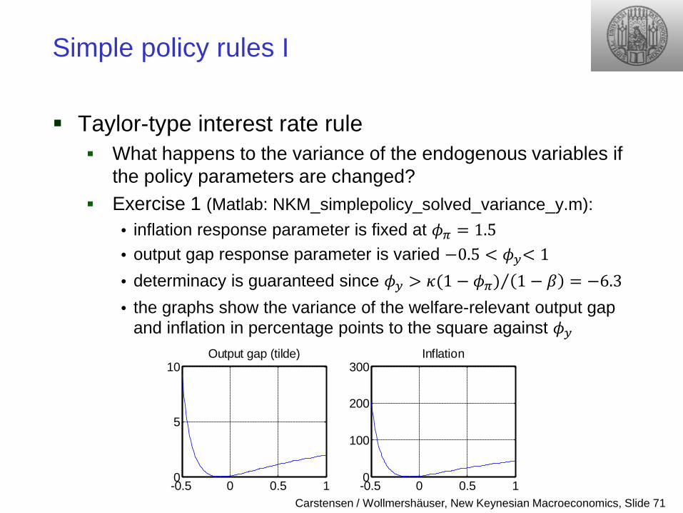
Taylor-type interest rate rule What happens to the variance of the endogenous variables if
the policy parameters are changed? Exercise 1 (Matlab: NKM_simplepolicy_solved_variance_y.m):
• inflation response parameter is fixed at 𝜙𝜋 = 1.5 • output gap response parameter is varied −0.5 < 𝜙𝑦< 1 • determinacy is guaranteed since 𝜙𝑦 > 𝜅(1 − 𝜙𝜋) 1 − 𝛽 = −6.3⁄ • the graphs show the variance of the welfare-relevant output gap
and inflation in percentage points to the square against 𝜙𝑦
-0.5 0 0.5 10
5
10Output gap (tilde)
-0.5 0 0.5 10
100
200
300Inflation
Carstensen / Wollmershäuser, New Keynesian Macroeconomics, Slide 72
Simple policy rules I
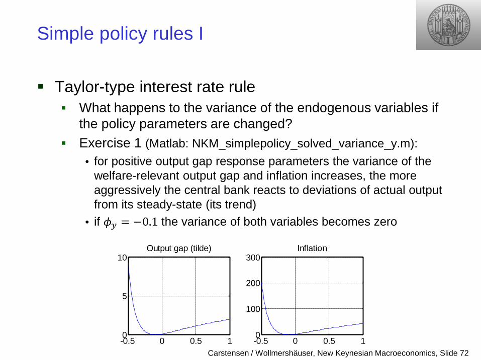
Taylor-type interest rate rule What happens to the variance of the endogenous variables if
the policy parameters are changed? Exercise 1 (Matlab: NKM_simplepolicy_solved_variance_y.m):
• for positive output gap response parameters the variance of the welfare-relevant output gap and inflation increases, the more aggressively the central bank reacts to deviations of actual output from its steady-state (its trend)
• if 𝜙𝑦 = −0.1 the variance of both variables becomes zero
-0.5 0 0.5 10
5
10Output gap (tilde)
-0.5 0 0.5 10
100
200
300Inflation
Carstensen / Wollmershäuser, New Keynesian Macroeconomics, Slide 73
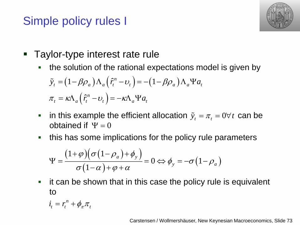
Simple policy rules I
Taylor-type interest rate rule the solution of the rational expectations model is given by
in this example the efficient allocation can be obtained if
this has some implications for the policy rule parameters
it can be shown that in this case the policy rule is equivalent to
( ) ( ) ( )
( )ˆ1 1
ˆ
nt a a t t a a t
nt a t t a t
y r a
r a
βρ υ βρ
π κ υ κ
= − Λ − = − − Λ Ψ
= Λ − = − Λ Ψ
0t ty tπ= = ∀
( ) ( )( )( ) ( )
1 10 1
1a y
y a
ϕ σ ρ φφ σ ρ
σ α ϕ α
+ − +Ψ = = ⇔ = − −
− + +
0Ψ =
nt t ti r πφ π= +
Carstensen / Wollmershäuser, New Keynesian Macroeconomics, Slide 74
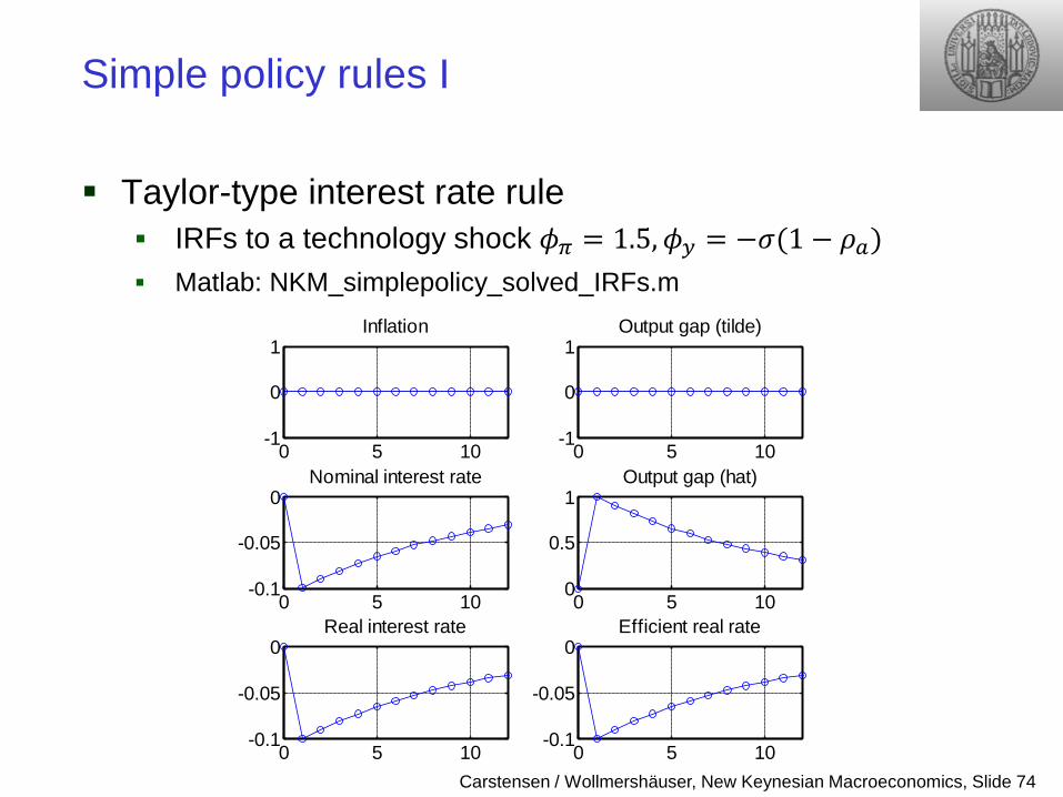
Simple policy rules I
Taylor-type interest rate rule IRFs to a technology shock 𝜙𝜋 = 1.5,𝜙𝑦 = −𝜎(1 − 𝜌𝑎) Matlab: NKM_simplepolicy_solved_IRFs.m
0 5 10-1
0
1Inflation
0 5 10-1
0
1Output gap (tilde)
0 5 10-0.1
-0.05
0Nominal interest rate
0 5 100
0.5
1Output gap (hat)
0 5 10-0.1
-0.05
0Real interest rate
0 5 10-0.1
-0.05
0Efficient real rate
Carstensen / Wollmershäuser, New Keynesian Macroeconomics, Slide 75
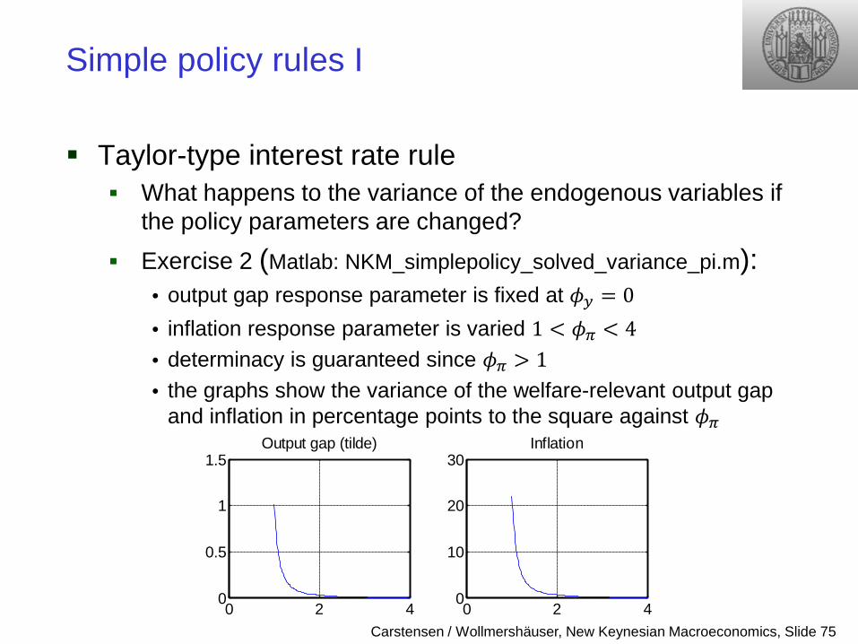
Simple policy rules I
Taylor-type interest rate rule What happens to the variance of the endogenous variables if
the policy parameters are changed? Exercise 2 (Matlab: NKM_simplepolicy_solved_variance_pi.m):
• output gap response parameter is fixed at 𝜙𝑦 = 0 • inflation response parameter is varied 1 < 𝜙𝜋 < 4 • determinacy is guaranteed since 𝜙𝜋 > 1 • the graphs show the variance of the welfare-relevant output gap
and inflation in percentage points to the square against 𝜙𝜋
0 2 40
0.5
1
1.5Output gap (tilde)
0 2 40
10
20
30Inflation
Carstensen / Wollmershäuser, New Keynesian Macroeconomics, Slide 76
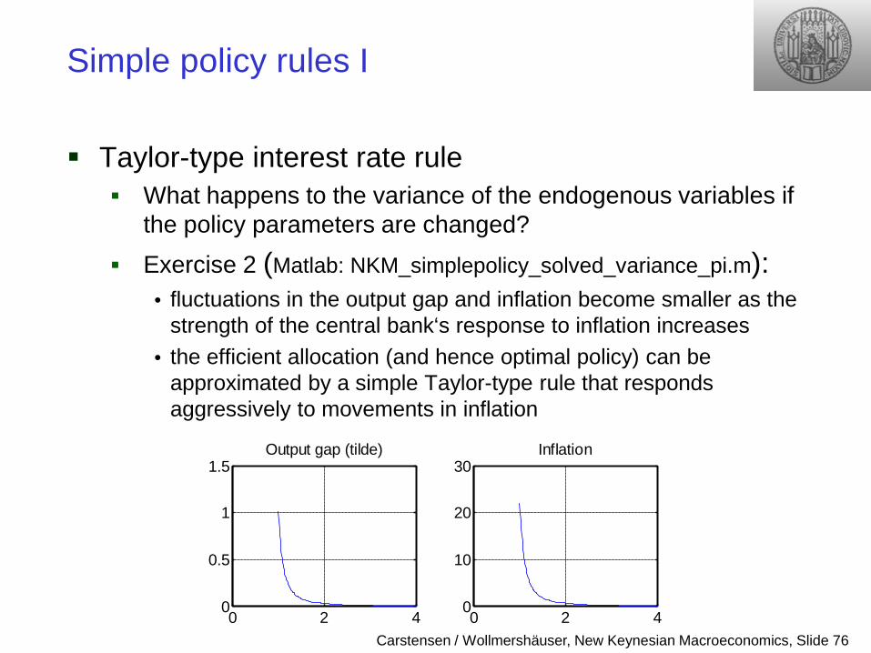
Simple policy rules I
Taylor-type interest rate rule What happens to the variance of the endogenous variables if
the policy parameters are changed? Exercise 2 (Matlab: NKM_simplepolicy_solved_variance_pi.m):
• fluctuations in the output gap and inflation become smaller as the strength of the central bank‘s response to inflation increases
• the efficient allocation (and hence optimal policy) can be approximated by a simple Taylor-type rule that responds aggressively to movements in inflation
0 2 40
0.5
1
1.5Output gap (tilde)
0 2 40
10
20
30Inflation