Embed Size (px)
Citation preview
Chapter 5 – Microlensing
PHY6795O – Chapitres Choisis en Astrophysique
Naines Brunes et Exoplanètes
2
Contents5.1 Introduction 5.2 Description 5.3 Caustic and critical curves5.4 Other light curve effects5.5 Microlens parallax and lens mass5.6 Astrometric microlensing5.7 Other configurations5.8 Microlensing observations in practice5.9 Exoplanet results5.10 Summary of limitations and strengths5.11 Future developments
5. MicrolensingPHY6795O – Naines brunes et Exoplanètes
3
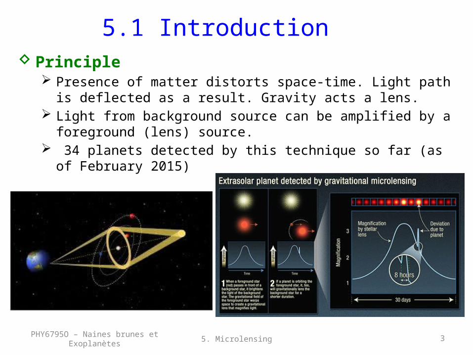
5.1 Introduction Principle
Presence of matter distorts space-time. Light path is deflected as a result. Gravity acts a lens.
Light from background source can be amplified by a foreground (lens) source.
34 planets detected by this technique so far (as of February 2015)
5. MicrolensingPHY6795O – Naines brunes et Exoplanètes
4
5.1 Introduction (2) Strong lensing
Effects discernable at an individual object level. Macrolensing: multiple resolved images, arcs,
distorted/amplified sources. Microlensing: discrete multiple images are unresolved.
• Relevant for exoplanet detection. • Requires extremely precise alignment of observer, source and
lens to within the angular Einstein radius, or ~1 mas.• Primary lens mass is of order 1 M.
• Intensity variation of primary lens time scale: several weeks• Secondary lens effect due to planet: several hours.• Very low probability of event. Requires 100s millions sources to
be monitored simultaneously.
5. MicrolensingPHY6795O – Naines brunes et Exoplanètes
5
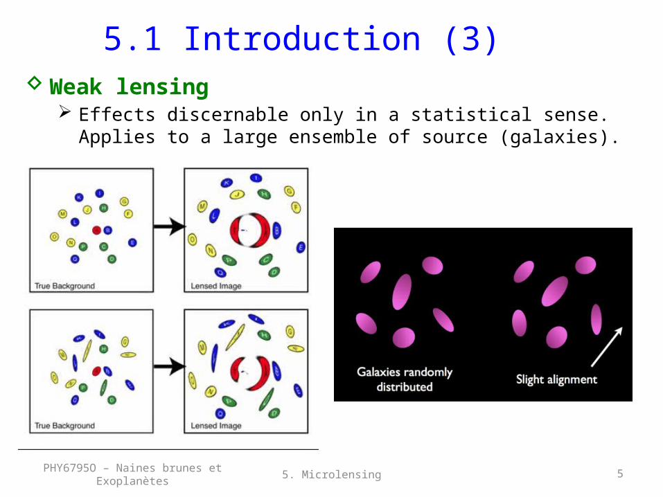
5.1 Introduction (3) Weak lensing
Effects discernable only in a statistical sense. Applies to a large ensemble of source (galaxies).
5. MicrolensingPHY6795O – Naines brunes et Exoplanètes
6
Contents5.1 Introduction 5.2 Description 5.3 Caustic and critical curves5.4 Other light curve effects5.5 Microlens parallax and lens mass5.6 Astrometric microlensing5.7 Other configurations5.8 Microlensing observations in practice5.9 Exoplanet results5.10 Summary of limitations and strengths5.11 Future developments
5. MicrolensingPHY6795O – Naines brunes et Exoplanètes
7
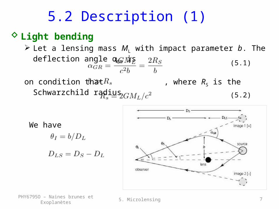
5.2 Description (1) Light bending
Let a lensing mass ML with impact parameter b. The deflection angle αGR is
on condition that , where RS is the Schwarzchild radius
We have
5. MicrolensingPHY6795O – Naines brunes et Exoplanètes
(5.1)
(5.2)
8
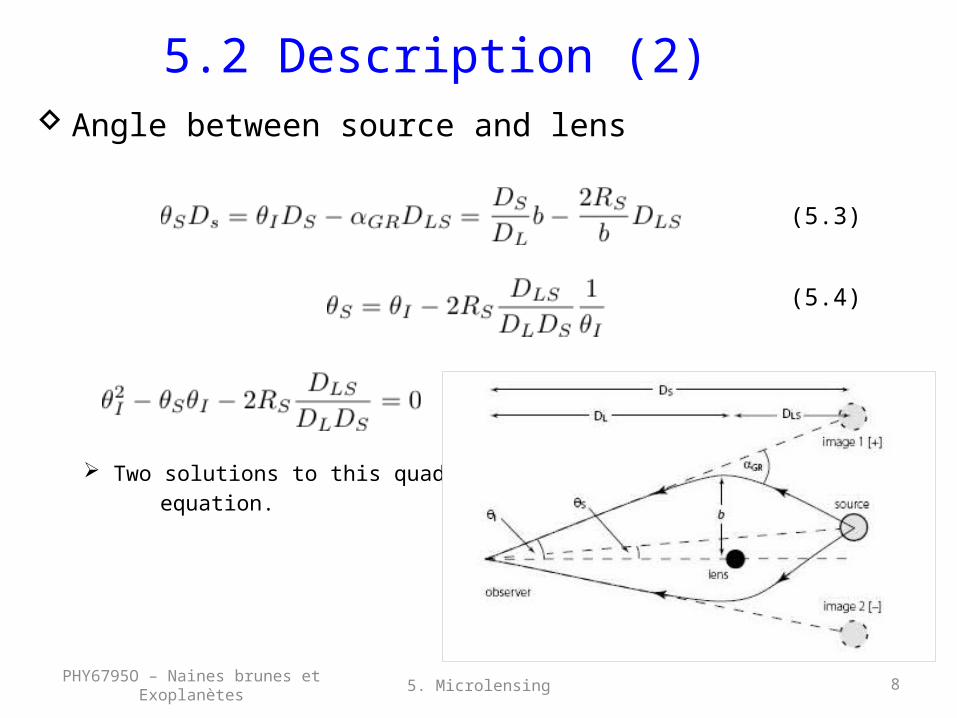
5.2 Description (2) Angle between source and lens
Two solutions to this quadratic equation.
5. MicrolensingPHY6795O – Naines brunes et Exoplanètes
(5.3)
(5.4)
9
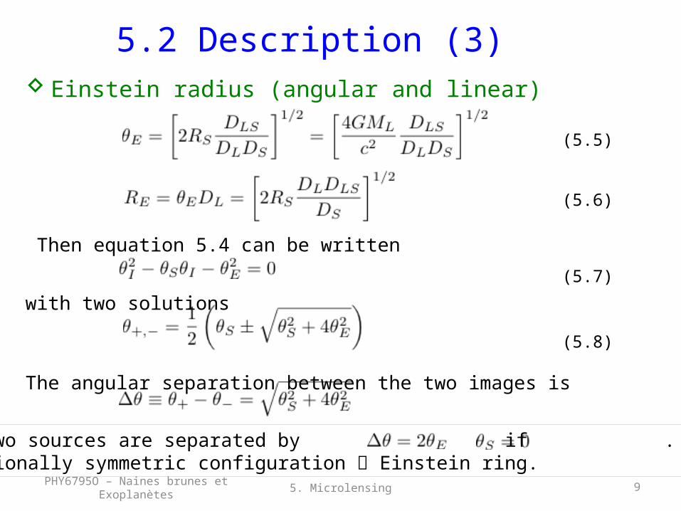
5.2 Description (3) Einstein radius (angular and linear)
Then equation 5.4 can be written
with two solutions
The angular separation between the two images is
5. MicrolensingPHY6795O – Naines brunes et Exoplanètes
(5.5)
(5.6)
(5.7)
(5.8)
The two sources are separated by if . Rotationally symmetric configuration Einstein ring.
10
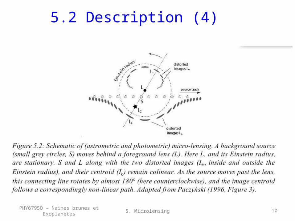
5.2 Description (4)
5. MicrolensingPHY6795O – Naines brunes et Exoplanètes
11
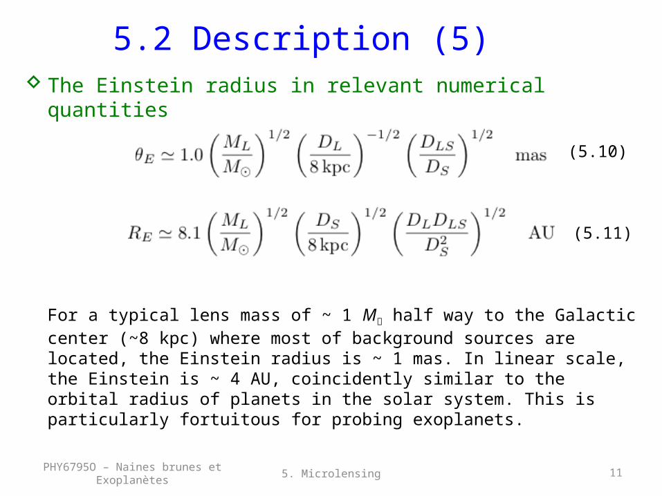
5.2 Description (5) The Einstein radius in relevant numerical quantities
For a typical lens mass of ~ 1 M half way to the Galactic center (~8 kpc) where most of background sources are located, the Einstein radius is ~ 1 mas. In linear scale, the Einstein is ~ 4 AU, coincidently similar to the orbital radius of planets in the solar system. This is particularly fortuitous for probing exoplanets.
5. MicrolensingPHY6795O – Naines brunes et Exoplanètes
(5.10)
(5.11)
12
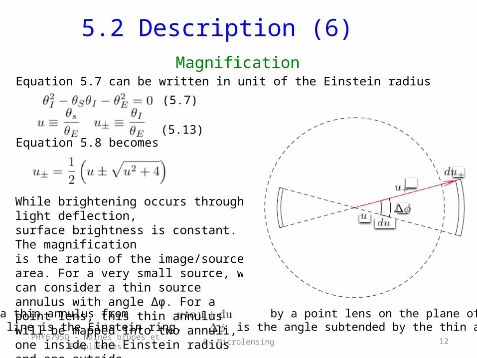
5.2 Description (6) Magnification
Equation 5.7 can be written in unit of the Einstein radius
Equation 5.8 becomes
5. MicrolensingPHY6795O – Naines brunes et Exoplanètes
(5.7)
While brightening occurs through light deflection,surface brightness is constant. The magnification is the ratio of the image/source area. For a very small source, we can consider a thin source annulus with angle Δϕ. For a point lens, this thin annulus will be mapped into two annuli, one inside the Einstein radius and one outside.
(5.13)
Images of a thin annulus from by a point lens on the plane of the sky.The dashed line is the Einstein ring. is the angle subtended by the thin annulus.
13
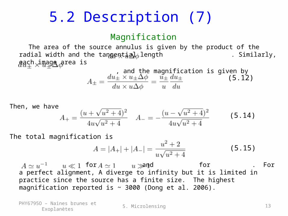
5.2 Description (7) Magnification
The area of the source annulus is given by the product of the radial width and the tangential length . Similarly, each image area is
, and the magnification is given by
Then, we have
The total magnification is
for and for . For a perfect alignment, A diverge to infinity but it is limited in practice since the source has a finite size. The highest magnification reported is ~ 3000 (Dong et al. 2006).
5. MicrolensingPHY6795O – Naines brunes et Exoplanètes
(5.12)
(5.14)
(5.15)
14
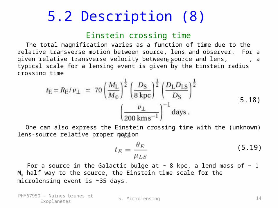
5.2 Description (8) Einstein crossing time
The total magnification varies as a function of time due to the relative transverse motion between source, lens and observer. For a given relative transverse velocity between source and lens, , a typical scale for a lensing event is given by the Einstein radius crossing time
One can also express the Einstein crossing time with the (unknown) lens-source relative proper motion
For a source in the Galactic bulge at ~ 8 kpc, a lend mass of ~ 1 M half way to the source, the Einstein time scale for the microlensing event is ~35 days.
5. MicrolensingPHY6795O – Naines brunes et Exoplanètes
(5.18)
(5.19)
15
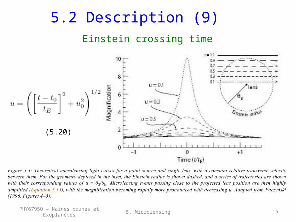
5.2 Description (9) Einstein crossing time
5. MicrolensingPHY6795O – Naines brunes et Exoplanètes
(5.20)
16
Contents5.1 Introduction 5.2 Description 5.3 Caustic and critical curves5.4 Other light curve effects5.5 Microlens parallax and lens mass5.6 Astrometric microlensing5.7 Other configurations5.8 Microlensing observations in practice5.9 Exoplanet results5.10 Summary of limitations and strengths5.11 Future developments
5. MicrolensingPHY6795O – Naines brunes et Exoplanètes
17
5.3 Caustics and critical curves (1) Critical curves are regions in the lens plane where the
magnification is infinite. Corresponding regions in the source plane as mapped by the lens equation are termed caustics.
For a single point lens, the caustic is the single point behind and the critical curves (positions of the images of these caustics) is the Einstein ring.
High-magnification microlensing events occur when the source comes near to a caustic.
For a binary lens, a star and an orbiting planet, the caustics and shapes can be formulated in terms of the planet/star ratio q=Mp/M★, the angular star-planet separation d in units of θE and α, the angle of the source trajectory relative to te binary axis. The planet induces a secondary peak in the smooth light curve. For
Earth-mass planets, the time scale of the secondary microlensing event is 3-5 hours.
5. MicrolensingPHY6795O – Naines brunes et Exoplanètes
18
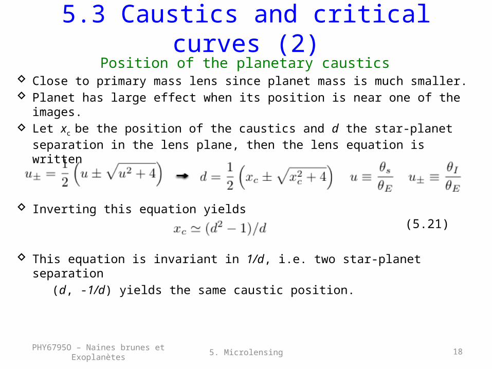
5.3 Caustics and critical curves (2)Position of the planetary caustics
Close to primary mass lens since planet mass is much smaller. Planet has large effect when its position is near one of the
images. Let xc be the position of the caustics and d the star-planet
separation in the lens plane, then the lens equation is written
Inverting this equation yields
This equation is invariant in 1/d, i.e. two star-planet separation (d, -1/d) yields the same caustic position.
5. MicrolensingPHY6795O – Naines brunes et Exoplanètes
(5.21)
19
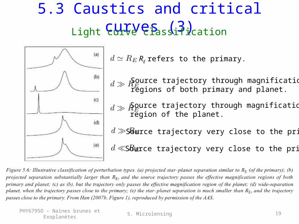
5.3 Caustics and critical curves (3)Light curve classification
5. MicrolensingPHY6795O – Naines brunes et Exoplanètes
Source trajectory through magnificationregion of the planet.
Source trajectory through magnificationregions of both primary and planet.
Source trajectory very close to the primary.
Source trajectory very close to the primary.
RE refers to the primary.
20
Contents5.1 Introduction 5.2 Description 5.3 Caustic and critical curves5.4 Other light curve effects5.5 Microlens parallax and lens mass5.6 Astrometric microlensing5.7 Other configurations5.8 Microlensing observations in practice5.9 Exoplanet results5.10 Summary of limitations and strengths5.11 Future developments
5. MicrolensingPHY6795O – Naines brunes et Exoplanètes
21
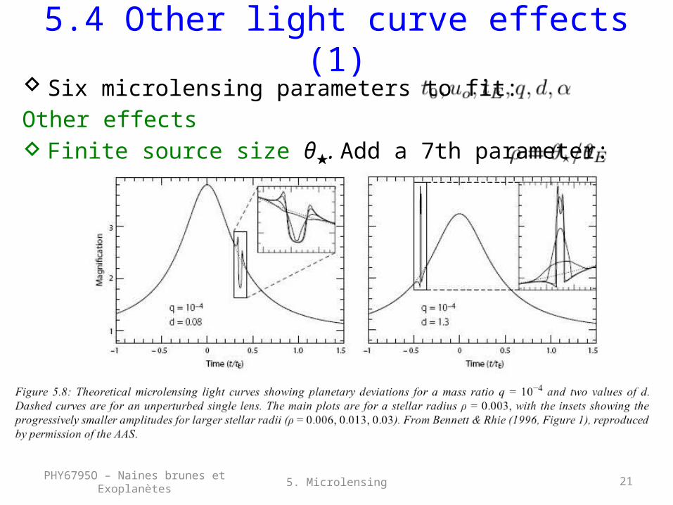
5.4 Other light curve effects (1) Six microlensing parameters to fit:Other effects Finite source size θ★. Add a 7th parameter:
5. MicrolensingPHY6795O – Naines brunes et Exoplanètes
22
5.4 Other light curve effects (2) Limb darkening and star spots Orbital motion of a binary lens
Three cases: rotating binary lens, rotating binary source and a rotating oberver (Earth orbiting the Sun)
Most dramatic effects for a rotating binary lens. First claimed planetary microlensing event MACHO-97-BLG-
41 was revised with an improved fit involving a binary with a period of 1.5 yr.
Orbital motion of a star-planet lens Effect seen in the data for the outer planet in the first
multiple planetary microlensing event, OGLE-2006-BLG-109L (Gaudi et al. 2008)
5. MicrolensingPHY6795O – Naines brunes et Exoplanètes
23
5.4 Other light curve effects (3) Blending
Due to a physical companion of the source star, lens itself or superposition of another (non-lensing) object along line-of-sight. Separation between light from source and lens is possible once angular separation has increased by a few mas, several years after the lens event. Difference in color between the source and the lens will result in a small displacement of the centroid with wavelength.• Yields an estimate of the host star spectral type and, with
assumption on underlying stellar population, DL, hence a complete solution to lens equation.
Relative source-lense transverse motion Cannot be determined from light curve but possible by measuring
small change in the elongation of the image, .e.g. with stable PSF from HST.• Yield the relative angular proper motion μLS, hence the Einstein radius
from equation 5.19.
5. MicrolensingPHY6795O – Naines brunes et Exoplanètes
24
Contents5.1 Introduction 5.2 Description 5.3 Caustic and critical curves5.4 Other light curve effects5.5 Microlens parallax and lens mass5.6 Astrometric microlensing5.7 Other configurations5.8 Microlensing observations in practice5.9 Exoplanet results5.10 Summary of limitations and strengths5.11 Future developments
5. MicrolensingPHY6795O – Naines brunes et Exoplanètes
25
5.5 Microlens parallax and lens mass (1)
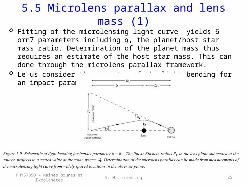
Fitting of the microlensing light curve yields 6 orn7 parameters including q, the planet/host star mass ratio. Determination of the planet mass thus requires an estimate of the host star mass. This can done through the microlens parallax framework.
Le us consider the geometry of the light bending for an impact parameter b=RE
5. MicrolensingPHY6795O – Naines brunes et Exoplanètes
26
5.5 Microlens parallax and lens mass (2)
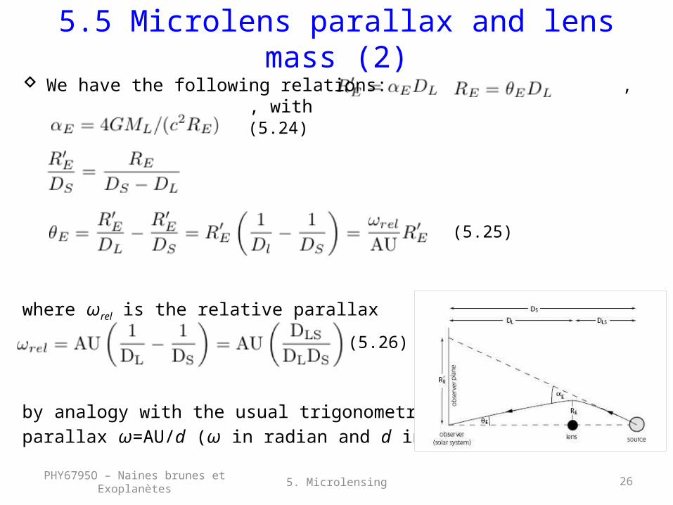
We have the following relations: , , with
where ωrel is the relative parallax
by analogy with the usual trigonometric parallax ω=AU/d (ω in radian and d in AU)
5. MicrolensingPHY6795O – Naines brunes et Exoplanètes
(5.24)
(5.25)
(5.26)
27
5.5 Microlens parallax and lens mass (3)
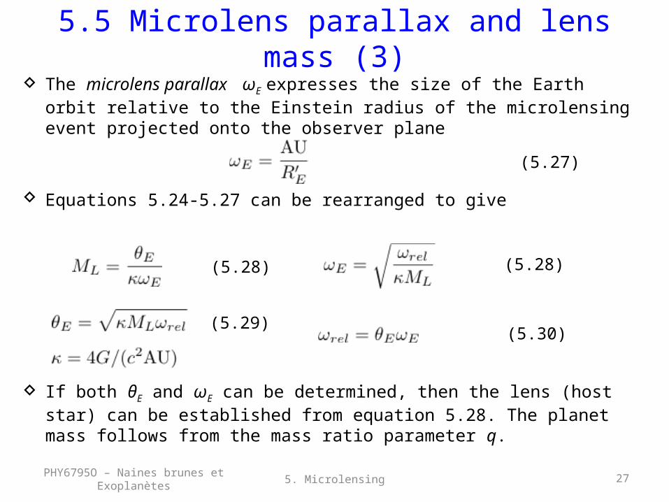
The microlens parallax ωE expresses the size of the Earth orbit relative to the Einstein radius of the microlensing event projected onto the observer plane
Equations 5.24-5.27 can be rearranged to give
If both θE and ωE can be determined, then the lens (host star) can be established from equation 5.28. The planet mass follows from the mass ratio parameter q.
5. MicrolensingPHY6795O – Naines brunes et Exoplanètes
(5.28)
(5.27)
(5.28)
(5.29)(5.30)
28
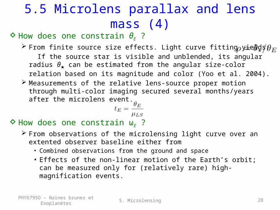
5.5 Microlens parallax and lens mass (4)
How does one constrain θE ? From finite source size effects. Light curve fitting yields: If the source star is visible and unblended, its angular radius θ★
can be estimated from the angular size-color relation based on its magnitude and color (Yoo et al. 2004).
Measurements of the relative lens-source proper motion through multi-color imaging secured several months/years after the microlens event.
How does one constrain ωE ? From observations of the microlensing light curve over an
extented observer baseline either from• Combined observations from the ground and space
• Effects of the non-linear motion of the Earth’s orbit; can be measured only for (relatively rare) high-magnification events.
5. MicrolensingPHY6795O – Naines brunes et Exoplanètes
29
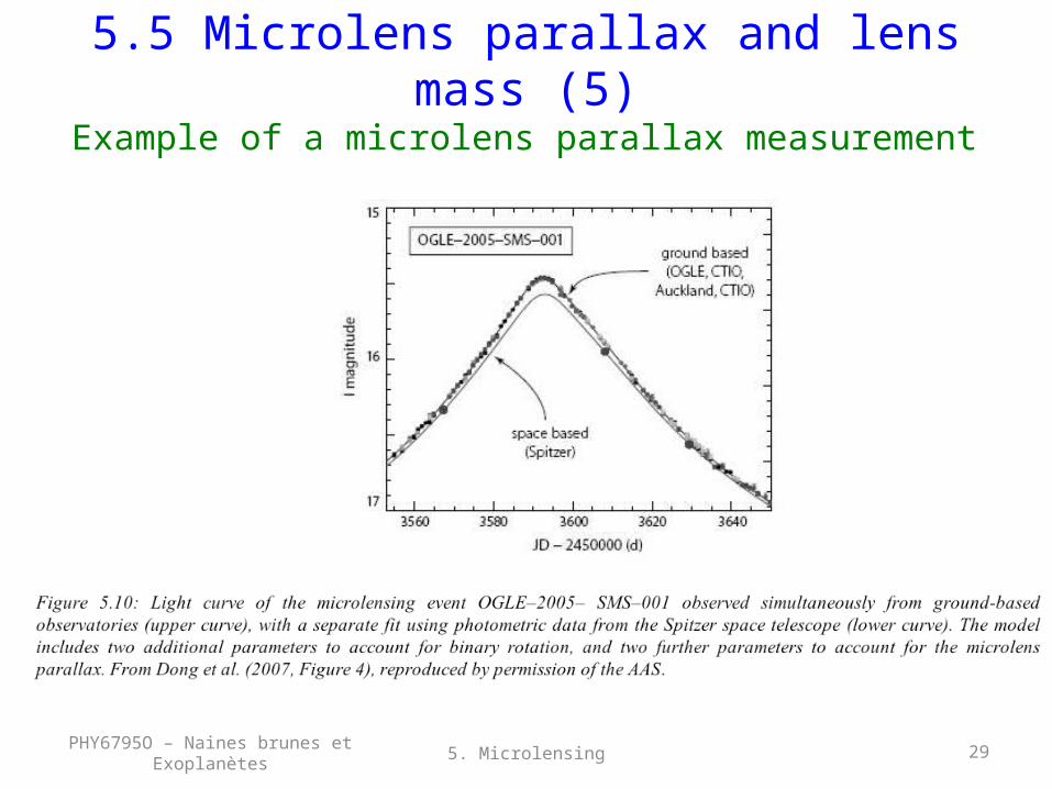
5.5 Microlens parallax and lens mass (5)
Example of a microlens parallax measurement
5. MicrolensingPHY6795O – Naines brunes et Exoplanètes
30
Contents5.1 Introduction 5.2 Description 5.3 Caustic and critical curves5.4 Other light curve effects5.5 Microlens parallax and lens mass5.6 Astrometric microlensing5.7 Other configurations5.8 Microlensing observations in practice5.9 Exoplanet results5.10 Summary of limitations and strengths5.11 Future developments
5. MicrolensingPHY6795O – Naines brunes et Exoplanètes
31
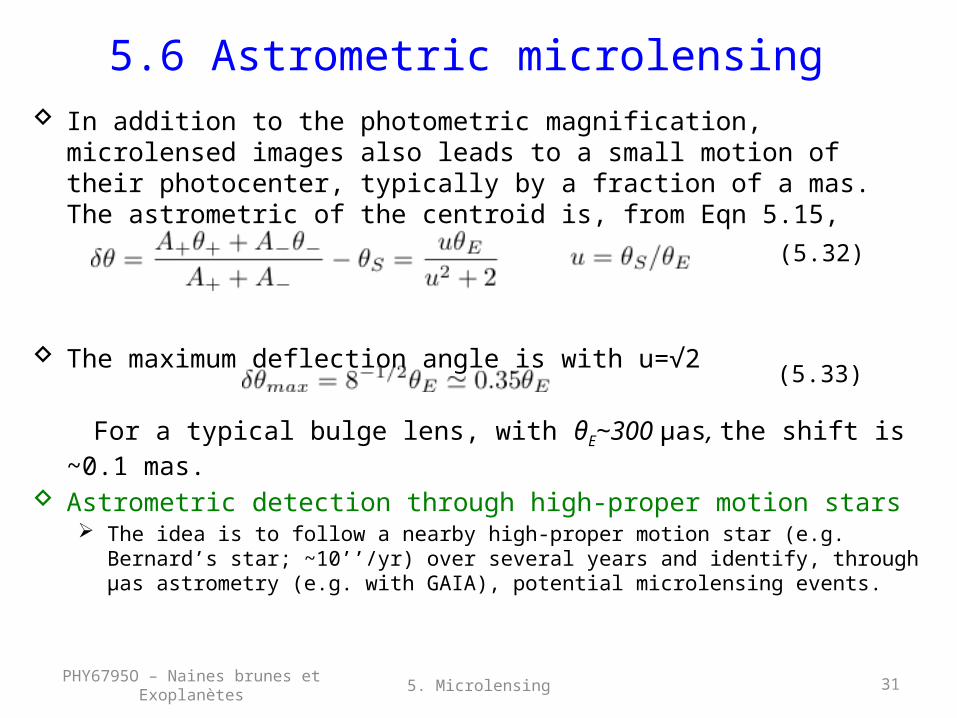
5.6 Astrometric microlensing In addition to the photometric magnification, microlensed
images also leads to a small motion of their photocenter, typically by a fraction of a mas. The astrometric of the centroid is, from Eqn 5.15,
The maximum deflection angle is with u=√2
For a typical bulge lens, with θE~300 μas, the shift is ~0.1 mas. Astrometric detection through high-proper motion stars
The idea is to follow a nearby high-proper motion star (e.g. Bernard’s star; ~10’’/yr) over several years and identify, through μas astrometry (e.g. with GAIA), potential microlensing events.
5. MicrolensingPHY6795O – Naines brunes et Exoplanètes
(5.32)
(5.33)
32
Contents5.1 Introduction 5.2 Description 5.3 Caustic and critical curves5.4 Other light curve effects5.5 Microlens parallax and lens mass5.6 Astrometric microlensing5.7 Other configurations5.8 Microlensing observations in practice5.9 Exoplanet results5.10 Summary of limitations and strengths5.11 Future developments
5. MicrolensingPHY6795O – Naines brunes et Exoplanètes
33
5.7 Other configurations
Other source/lens configurations that might be observed in the future.
Planet orbiting the source star. Provides information on atmospheric composition, satellites
and ring. Planets could be detected as they cross the caustics of the foreground lens. Theoretically possible to detect H2O and CH4 of a close-in Jupiter (Spiegel et al. 2005).
Satellite orbiting a planet Feasible under favourable conditions.
Planet orbiting a binary system Free-floating planets Microlensed transiting planets Planetasimal disks
5. MicrolensingPHY6795O – Naines brunes et Exoplanètes
34
Contents5.1 Introduction 5.2 Description 5.3 Caustic and critical curves5.4 Other light curve effects5.5 Microlens parallax and lens mass5.6 Astrometric microlensing5.7 Other configurations5.8 Microlensing observations in practice5.9 Exoplanet results5.10 Summary of limitations and strengths5.11 Future developments
5. MicrolensingPHY6795O – Naines brunes et Exoplanètes
35
5.8 Microlensing in practice Large-scale observing programmes focus on Baades’s Window
in the central Galactic bulge. Pros: high stellar density to maximize number of microlensing events.
Region of relatively low extinction. Cons: crowding and blending.
Observing strategy: Two-step mode1. Wide-angle survey detects the early stages of a microlensing event
using relatively coarse temporal sampling.2. Once deviation is significant, an alert is issued and an array of smaller,
follow-up narrow-angle telescopes distributed in Earth longitudes follow the events with high-precision photometry and a much denser time coverage.
Two major teams MOA (Microlensing Observations in Astrophysics); NZ/Japan
• Phase I: 0.6m telescope; Phase II: 2m telescope. 20 sq degrees. OGLE (Optical Gravitational Lens Experiment)
• 1.3m telescope in Chile Plus several teams for follow-up observations
5. MicrolensingPHY6795O – Naines brunes et Exoplanètes
36
Contents5.1 Introduction 5.2 Description 5.3 Caustic and critical curves5.4 Other light curve effects5.5 Microlens parallax and lens mass5.6 Astrometric microlensing5.7 Other configurations5.8 Microlensing observations in practice5.9 Exoplanet results5.10 Summary of limitations and strengths5.11 Future developments
5. MicrolensingPHY6795O – Naines brunes et Exoplanètes
37
5.9 Exoplanet results (1) Naming convention
After the team who first reported the event (ex: OGLE-2003-BLG-235)
The lens and source can be specified with the suffixes ‘L’ and ‘S’. Additioncal capital or lower case letters designate companions of stellar or planetary mass respectively• OGLE-2006-BLG-109LA, …Lb, …Lc designate specifically the star,
and the two known planets of this multiple system.
First detection: OGLE-2003-BLG-235 (Bond et al. 2004) Original etsimates: Mp~1.5 MJ, DL=5.2 kpc refined to Mp~2.6 MJ,
DL=5.8 kpc, after follow-up HST observations to constrain spectral type of the host (K) star.
First low-mass microlensing event (Beaulieu et al. 2006) Mp~5.5 ME, DL=6.6 kpc, M host.
5. MicrolensingPHY6795O – Naines brunes et Exoplanètes
38
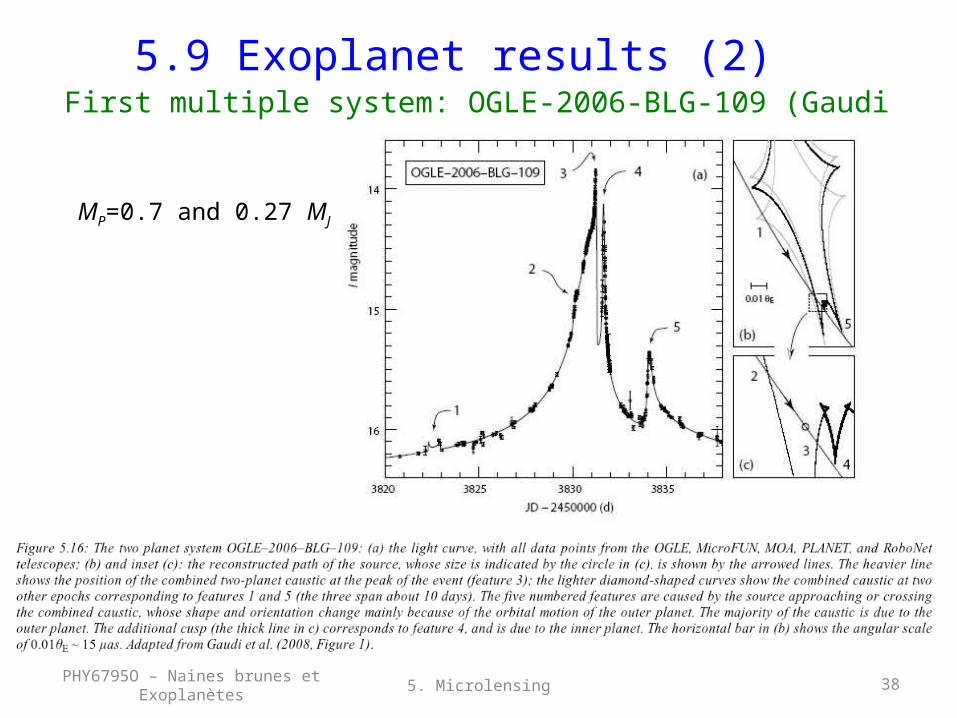
5.9 Exoplanet results (2) First multiple system: OGLE-2006-BLG-109 (Gaudi etal.
2008)
5. MicrolensingPHY6795O – Naines brunes et Exoplanètes
MP=0.7 and 0.27 MJ
39
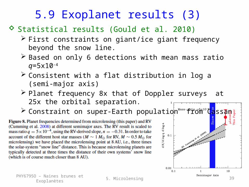
5.9 Exoplanet results (3) Statistical results (Gould et al. 2010)
First constraints on giant/ice giant frequency beyond the snow line.
Based on only 6 detections with mean mass ratio q=5x10⁻⁴
Consistent with a flat distribution in log a (semi-major axis) Planet frequency 8x that of Doppler surveys at 25x the
orbital separation. Constraint on super-Earth population from Cassan et al.
(2012).
5. MicrolensingPHY6795O – Naines brunes et Exoplanètes
40
Contents5.1 Introduction 5.2 Description 5.3 Caustic and critical curves5.4 Other light curve effects5.5 Microlens parallax and lens mass5.6 Astrometric microlensing5.7 Other configurations5.8 Microlensing observations in practice5.9 Exoplanet results5.10 Summary of limitations and strengths5.11 Future developments
5. MicrolensingPHY6795O – Naines brunes et Exoplanètes
41
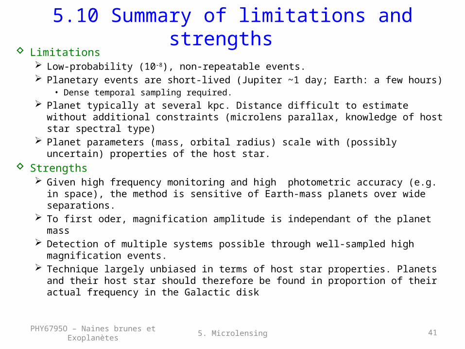
5.10 Summary of limitations and strengths
Limitations Low-probability (10-8), non-repeatable events. Planetary events are short-lived (Jupiter ~1 day; Earth: a few hours)
• Dense temporal sampling required. Planet typically at several kpc. Distance difficult to estimate without
additional constraints (microlens parallax, knowledge of host star spectral type)
Planet parameters (mass, orbital radius) scale with (possibly uncertain) properties of the host star.
Strengths Given high frequency monitoring and high photometric accuracy (e.g. in
space), the method is sensitive of Earth-mass planets over wide separations.
To first oder, magnification amplitude is independant of the planet mass Detection of multiple systems possible through well-sampled high
magnification events. Technique largely unbiased in terms of host star properties. Planets and
their host star should therefore be found in proportion of their actual frequency in the Galactic disk
5. MicrolensingPHY6795O – Naines brunes et Exoplanètes
42
Contents5.1 Introduction 5.2 Description 5.3 Caustic and critical curves5.4 Other light curve effects5.5 Microlens parallax and lens mass5.6 Astrometric microlensing5.7 Other configurations5.8 Microlensing observations in practice5.9 Exoplanet results5.10 Summary of limitations and strengths5.11 Future developments
5. MicrolensingPHY6795O – Naines brunes et Exoplanètes
43
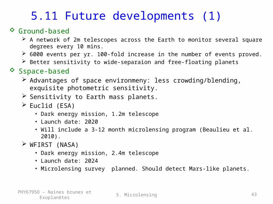
5.11 Future developments (1) Ground-based
A network of 2m telescopes across the Earth to monitor several square degrees every 10 mins.
6000 events per yr. 100-fold increase in the number of events proved. Better sensitivity to wide-separaion and free-floating planets
Sspace-based Advantages of space environmeny: less crowding/blending,
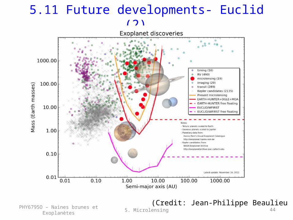
exquisite photometric sensitivity. Sensitivity to Earth mass planets. Euclid (ESA)
• Dark energy mission, 1.2m telescope• Launch date: 2020• Will include a 3-12 month microlensing program (Beaulieu et al. 2010).
WFIRST (NASA)• Dark energy mission, 2.4m telescope• Launch date: 2024• Microlensing survey planned. Should detect Mars-like planets.
5. MicrolensingPHY6795O – Naines brunes et Exoplanètes
44
5.11 Future developments- Euclid (2)
5. MicrolensingPHY6795O – Naines brunes et Exoplanètes(Credit: Jean-Philippe Beaulieu
45
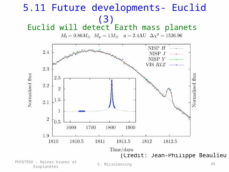
5.11 Future developments- Euclid (3)
5. MicrolensingPHY6795O – Naines brunes et Exoplanètes
Euclid will detect Earth mass planets
(Credit: Jean-Philippe Beaulieu
46
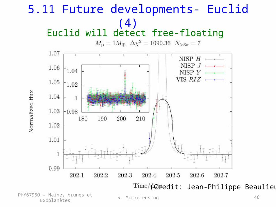
5.11 Future developments- Euclid (4)
5. MicrolensingPHY6795O – Naines brunes et Exoplanètes
Euclid will detect free-floating planets
(Credit: Jean-Philippe Beaulieu