1

Chapter 5 Managing Process Constraints

Theory of Constraints

Managing Bottlenecks

Assembly Line Balancing

What is a Constraint?

Constraint: Any factor that limits the performance of a system and restricts its output.

Bottleneck: A capacity constraint resource (CCR) whose available capacity limits the organization’s ability to meet the product volume, product mix, or demand fluctuations required by the marketplace

Supply Operation 1 20/hr.

Operation 2 12/hr.

Operation 3 16/hr. Demand

2

Operational Measures vs. Financial Measures

U↗  T↗  profit & ROI↗

Theory of Constraints

The focus should be on balancing flow, not on balancing capacity.

Maximizing the output and efficiency of every resource may not maximize the throughput of the entire system.

An hour lost at a bottleneck... is an hour lost for the whole system. An hour saved at a non‐bottleneck resource is a mirage.

Inventory is needed only in front of bottlenecks and in front of assembly and shipping points.

Work should be released into the system only as frequently as needed by the bottlenecks. Bottleneck flows should be equal to market demand

Activating a non‐bottleneck resource… doesn’t increase throughput or promote better performance.

Every capital investment must be viewed from the perspective of the global impact on overall throughput, inventory, and operating expense.

3

Implementation of The Theory of Constraints

1. Identify the System Bottleneck(s)

2. Exploit the Bottleneck(s): Maximize the throughput of the bottleneck(s).

3. Subordinate All Other Decisions to Step 2: Non‐bottleneck resources should be scheduled to support the bottleneck.

4. Elevate the Bottleneck(s): Try to increase the capacity of the bottleneck

5. Do Not Let Inertia Set In: Repeat steps 1–4 in order to identify and manage the new set of constraints.

Managing Bottlenecks in Service Processes

Throughput time: Total elapsed time from the start to the finish of a job or a customer being processed at one or more work centers

Example 5.1

How many approved loans can be processed in a 5‐hour work day?

4

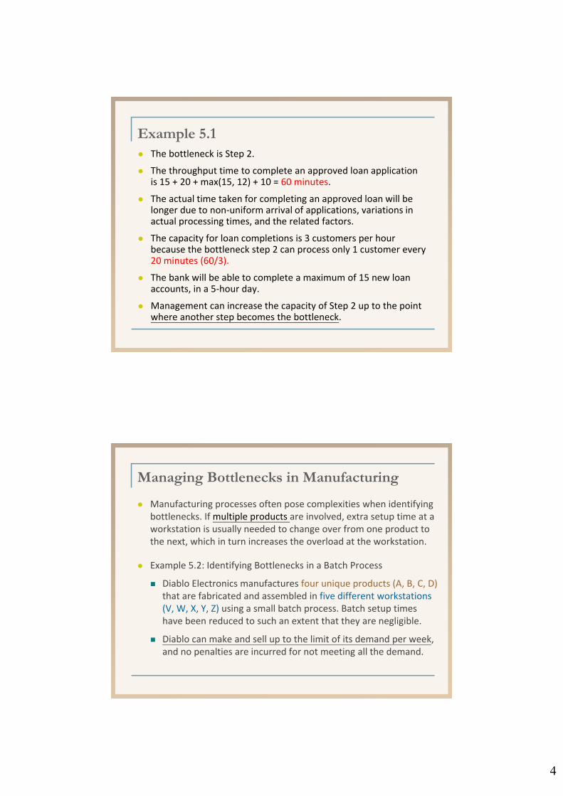
Example 5.1 The bottleneck is Step 2.

The throughput time to complete an approved loan application is 15 + 20 + max(15, 12) + 10 = 60 minutes. 

The actual time taken for completing an approved loan will be longer due to non‐uniform arrival of applications, variations in actual processing times, and the related factors.

The capacity for loan completions is 3 customers per hour because the bottleneck step 2 can process only 1 customer every 20 minutes (60/3).

The bank will be able to complete a maximum of 15 new loan accounts, in a 5‐hour day.

Management can increase the capacity of Step 2 up to the point where another step becomes the bottleneck.

Managing Bottlenecks in Manufacturing

Manufacturing processes often pose complexities when identifying bottlenecks. If multiple products are involved, extra setup time at a workstation is usually needed to change over from one product to the next, which in turn increases the overload at the workstation. 

Example 5.2: Identifying Bottlenecks in a Batch Process

Diablo Electronics manufactures four unique products (A, B, C, D)that are fabricated and assembled in five different workstations (V, W, X, Y, Z) using a small batch process. Batch setup times have been reduced to such an extent that they are negligible. 

Diablo can make and sell up to the limit of its demand per week, and no penalties are incurred for not meeting all the demand.

5

Product A

$5Raw materials

Purchased parts

Product APrice: $75/unitDemand: 60 units/week

Step 1 at workstation V

(30 min)

Step 3at workstation

X (10 min)

Step 2 atworkstation Y

(10 min)$5

Product C

Raw materialsPurchased parts

Product CPrice: $45/unitDemand:80 units/week

Step 4at workstation

Y(5 min)

Step 2 atworkstation Z

(5 min)

Step 3 atworkstation

X(5 min)

Step 1 atworkstation W

(5 min)

$2

$3

Product B

Raw materialsPurchased parts

Product BPrice: $72/unitDemand:80 units/week

Step 2at workstation X

(20 min)

Step 1 atworkstation Y

(10 min)$3

$2

Product D

Raw materialsPurchased parts

Product DPrice: $38/unitDemand:100 units/week

$4Step 2 at

workstation Z(10 min)

Step 3at workstation Y

(5 min)

Step 1 atworkstation W

(15 min)

$6

Example 5.2

Identifying bottlenecks becomes harder when setup times are lengthy and the degree of divergence in the process is greater. … floating bottlenecks

WorkstationLoad from Product A

Load from Product B

Load from Product C

Load from Product D

Total Load (min)

V

W

X

Y

Z

6030 = 1800 0 0 0 1,800

0 0 805 = 400 10015 = 1,500 1,900

Each week consists of 2,400 minutes of available production time. 

6010 = 600 8020 =1,600 0 2,600805 = 400

6010 = 600 8010 =800 1005 = 500 2,300

0 0 10010 = 1,000 1,400

805 = 400

805 = 400

6

Drum-Buffer-Rope Systems

Drum‐Buffer‐Rope: A planning and control system that regulates the flow of work‐in‐process materials at the bottleneck or the capacity constrained resource (CCR) in a productive system

The bottleneck schedule is the drum because it sets the beat or the production rate for the entire plant and is linked to market demand.

The buffer is the time buffer that plans early flows into the bottleneck and thus protects it from disruption.

The rope represents the tying of material release to the drum beat, which is the rate at which the bottleneck controls the throughput of the entire plant.

Applying TOC to Product Mix Decisions

Example 5.3: The management at Diablo Electronics wants to improve profitability by accepting the right set of orders (product mix). 

They collected the following financial data: 

Variable overhead costs are $8,500 per week. 

Each worker is paid $18 per hour and is paid for an entire week, regardless of how much the worker is used. 

Labor costs are fixed expenses. 

The plant operates one 8‐hour shift per day, or 40 hours each week. 

7

Example 5.3

Step 1: Calculate the contribution margin per unit of each product.

The order of the contribution margin per unit is B, A, C, D.

$75.00 $72.00 $45.00 $38.00

–10.00 –5.00 –5.00 –10.00

$65.00 $67.00 $40.00 $28.00

A B C D

Price

Raw material and purchased parts

= Contribution margin

Traditional Method: accept as much of the highest contribution margin product as possible (up to the limit), followed by the next highest contribution margin product, and so on until no more capacity is available. 

Example 5.3

Step 2: Allocate resources V, W, X, Y, and Z to the products in the order decided in Step 1. Satisfy each demand until the bottleneck resource (workstation X) is encountered. 

Work Center

Minutes at the Start

Minutes Left After Making 80 B

Minutes Left After Making 60 A

Can Only Make 40 C

Can Only Make 100 D

V

W

X

Y

Z

Step 3: Profit=(8067+6065+4040+10028) – (3600+8500)=1560

2,400

2,400

2,400

2,4002,400

2,4002,400

2,400

2,400

2,400

800

1,600

600

200

1,000 800

2,200

2,200

600

0

600700

0

3001,200

B(80):Y10, X20 A(60): V30, Y10, X10 C(80):W5, Z5, X5, Y5 D(100):W15, Z10, Y5

8

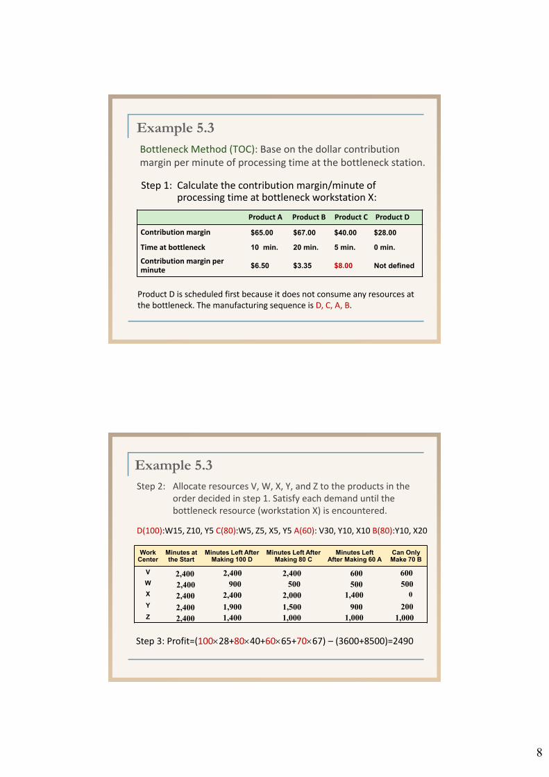
Product A Product B Product C Product D

Contribution margin

Time at bottleneck

Contribution margin per minute

Example 5.3

Bottleneck Method (TOC): Base on the dollar contribution margin per minute of processing time at the bottleneck station. 

$65.00 $67.00 $40.00 $28.00

10 min. 20 min. 5 min. 0 min.

$6.50 $3.35 $8.00 Not defined

Step 1: Calculate the contribution margin/minute of processing time at bottleneck workstation X:

Product D is scheduled first because it does not consume any resources at the bottleneck. The manufacturing sequence is D, C, A, B. 

Example 5.3Step 2: Allocate resources V, W, X, Y, and Z to the products in the 

order decided in step 1. Satisfy each demand until the bottleneck resource (workstation X) is encountered. 

Work Center

Minutes at the Start

Minutes Left After Making 100 D

Minutes Left After Making 80 C

Minutes Left After Making 60 A

Can Only Make 70 B

V

W

X

Y

Z

2,4002,4002,400

2,4002,400

2,400900

1,400

500

1,000

2,400

1,900

2,400

2,000

1,500 900

500

1,000

600

1,400

600500

0

2001,000

Step 3: Profit=(10028+8040+6065+7067) – (3600+8500)=2490

D(100):W15, Z10, Y5 C(80):W5, Z5, X5, Y5 A(60): V30, Y10, X10 B(80):Y10, X20 

9

Work Element Description Time (sec) Immediate

Predecessor(s)

A Bolt leg frame to hopper 40 None

B Insert impeller shaft 30 A

C Attach axle 50 A

D Attach agitator 40 B

E Attach drive wheel 6 B

F Attach free wheel 25 C

G Mount lower post 15 C

H Attach controls 20 D, E

I Mount nameplate 18 F, G

Total 244

Managing Constraints in a Line Process

Example 5.4: Green Grass, Inc. is designing an assembly line to produce a new fertilizer spreader. 

Precedence Diagram for Example 5.4

One worker for each step9 workers are needed.Output rate = one unit every 50 sec. = 72 units/hour

One worker for all stepsOutput rate = one unit every 244 sec. = 14.75 units/hour

10

Line Balancing 1/3

The assignment of work to stations in a line so as to achieve the desired output rate with the smallest number of workstations.

Assume r is the desired output rate matched to the production plan

Cycle time: Maximum time allowed for process a unit at each station to achieve the desired output rate r. c =

1

r

Theoretical Minimum (TM): the smallest number of stations possible to achieve the desired output rate r.

TM = tc

where  t = total time required to assemble each unit

Line Balancing 2/3

11

Line Balancing 3/3

Idle time = nc – t

where n =number of stations, c = cycle time, t =total time required to assemble each unit

Efficiency: the ratio of productive time to total time

Balance Delay: the amount by which efficiency falls short of 100%

Efficiency (%) =  (100) tnc

Balance delay (%) = 100 – Efficiency

Example 5.5

Green Grass’s plant manager just received marketing’s latest forecasts of Big Broadcaster sales for the next year. She wants its production line to be designed to make 2,400 spreaders per week. The plant will operate 40 hours per week.

a. What should be the line’s cycle time?

b. What is the smallest number of workstations that she could hope for in designing the line for this cycle time?

c. Suppose that she finds a solution that requires only five stations. What would be the line’s efficiency?

12

Example 5.5

a. First convert the desired output rate (2,400 units per week) to an hourly rate of 60. Then the cycle time is

c = 1/r =

b. Calculate the theoretical minimum for the number of stations by dividing the total time, t, by the cycle time, c = 60 sec. 

TM = tc

244 seconds

60 seconds=                     = 4.067 or 5 stations

1/60 (hr/unit) = 1 minute/unit = 60 seconds/unit

The number of stations is at least 5.

Example 5.5

1. Start with A. → Station 1

2. Use longest work element rule to select C. → Station 2

3. Use most followers rule to select B. → Station 33.1 Add F to Station 3.

4. Use longest work element rule to select D. → Station 44.1 Add G to Station 4.

5. Use most followers rule to select E. → Station 55.1 Add H and I to Station 5.

The precedence and cycle‐time requirements can not be violated.

13

Example 5.5

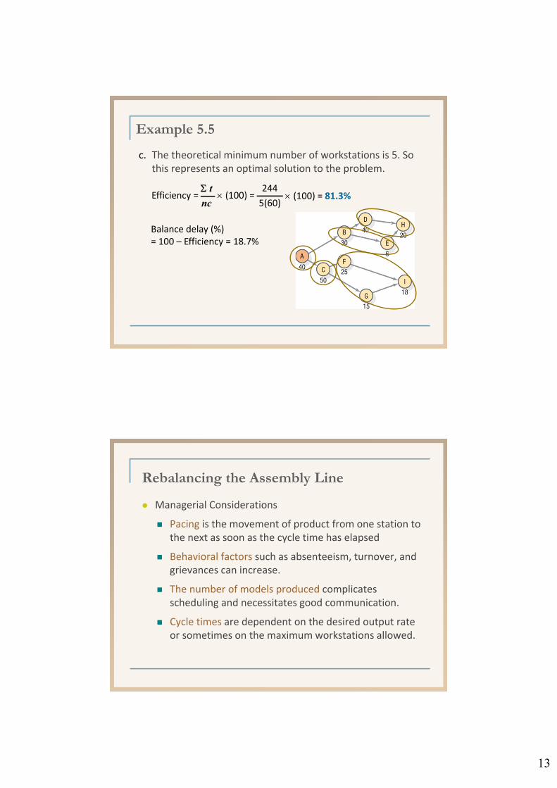
c. The theoretical minimum number of workstations is 5. So this represents an optimal solution to the problem.

Efficiency =         (100) = tnc

244

5(60) (100) = 81.3%

Balance delay (%) = 100 – Efficiency = 18.7%

Rebalancing the Assembly Line

Managerial Considerations

Pacing is the movement of product from one station to the next as soon as the cycle time has elapsed

Behavioral factors such as absenteeism, turnover, and grievances can increase.

The number of models produced complicates scheduling and necessitates good communication.

Cycle times are dependent on the desired output rate or sometimes on the maximum workstations allowed.