96

CHAPTER 5

33 Some of the work presented in this section was first presented in Rocha[1991].

34 Nakamura and Iwai’s work has been expanded formally and in its interpretation from itsoriginal form.

97

IMPLEMENTING CONTEXTUAL STRUCTURES FOR DATA MININGIn this chapter the formalisms defined in chapters 3 and 4 are explored computationally. The

applications developed pertain to the broad field of data mining. This area of Information Sciences andMachine Learning is dedicated to building computational tools that can help us search and categorize theimmense information resources available today. One of the most significant subareas of data mining researchis that of knowledge discovery in databases. Particularly with the exponential growth of the Internet, it isbecoming harder and harder to effectively search databases without being overwhelmed by a cascade ofunrelated results to users’ queries. Section 1 of this chapter presents a conversational knowledge discoverysystem for relational databases that uses evidence sets as categorization mechanisms. Its objective is thedefinition of a human-machine interface that can capture more efficiently the user’s interests through aninteractive question-answering process.

Another area of interest to data mining is that of the search of solutions for a problem in very largestate spaces. Contextual genetic algorithms (CGA’s) with fuzzy indirect encoding are used in two differentproblems. The first is the search of the appropriate set of weights for a very large Neural Network. The GAis used as a learning algorithm. It is a continuous variable problem. The second problem is the evolution ofCellular Automata rules to solve non-trivial tasks. It is a discrete variable problem. The fuzzy indirectencoding CGA of chapter 4 is shown to deal with such large problems efficiently.

1. Computing Categories in Relational Databases: Linguistic Categories asConsensual Selection of Dynamics33

The notion of uncertainty, is very relevant to any discussion of the modeling of linguistic/mentalabilities. From Zadeh's [1971, 1975] approximate reasoning to probabilistic and even evidential reasoning[Schum, 1994], uncertainty is more and more recognized as a very important issue in cognitive science andartificial intelligence with respect to the problems of knowledge representation and the modeling ofreasoning abilities [Shafer and Pearl, 1990]. Engineers of knowledge based systems can no longer be solelyconcerned with issues of linguistic or cognitive representation, they must describe "reasoning" procedureswhich enable an artificial system to answer queries. In many artificial intelligence systems, the choice of thenext step in a reasoning procedure is based upon the measurement of the system’s current uncertainty state[Nakamura and Iwai, 1982; Medina-Martins et al, 1992, 1994]. Now that a theory of evidential approximatereasoning and measures of uncertainty are defined for evidence sets (see chapter 3), we can extend fuzzydata-retrieval systems to an evidence set formulation.

1.1 Nakamura and Iwai’s Fuzzy Information Retrieval System34

Nakamura and Iwai’s [1982] data-retrieval system is based on a structure with two different kindsof objects: Concepts xi (e.g. Keywords) and Properties pi (e.g. data records like books). Each concept isassociated with a number of properties which may be shared with other concepts. Based on the amount ofproperties shared with one another, a measure of similarity, s, can be constructed for concepts xi and xj:

35 This measure of distance calculated in a large network of nodes, is usually not a Euclideanmetric because it does not observe the triangular inequality. In other words, the shortest distance betweentwo nodes of the network might not be the direct path. This means that two nodes may be closer to eachother when another node is associated with them. Such measures of distance are referred to as semi-metrics [Galvin and Shore, 1991]. For the purposes of the work here presented, we do not need to worryabout the mathematical significance of semi-metrics.

98

s(xi,xj) N(xiBxj)

N(xiAxj)

N(xiBxj)

N(xi)�N(xj)N(xiBxj)(1)

d(xi,xj) 1

s(xi,xj)(2)

Figure 1: Structure of Nakamura and Iwai’sdatabase. A measure of distance is calculatedbetween concepts according to the number ofproperties in common.

where:

� N(xi) represents the number of properties that directly qualify concept xi.� N(xi�xj) represents the number of properties that directly qualify both xi and xj.� N(xiFxj) represents the number of properties that directly qualify either xi or xj.

The inverse of the similarity, s, creates a measure (semi-metric) of distance35, d (figure 1):

Naturally, some concepts will not share anyproperties between them. Several approaches can bepursued to calculate the distance between every conceptin the network. Nakamura and Iwai propose theunfolding of the structure starting at any two concepts,and digging into deeper levels until common propertiesare reached. Instead of this, I use an algorithm thatcalculates the shortest path between two concepts. First,the distances between directly linked concepts arecalculated using (2). After this, the shortest path iscalculated between indirectly linked concepts. To speedup the process, the algorithm allows the search ofindirect distances up to a certain level. The set of n-reachable concepts from concept xi, is the set ofconcepts that have no more that n direct paths between them. Thus if xi is directly linked to xj which is turndirectly linked to xk, then xk is a 2-reachable concept of xi. If we set the algorithm to paths up to level n, allconcepts that are only reachable in more than n direct paths from xi will have their distance to xi set toinfinity. The larger the network of concepts and properties, the larger is the need to have a small n to avoidlengthy computations.

1.1.1 The Long-Term Networked Memory Structure: Semantic Closure

99

After calculating the distances between concepts, a substructure can be recognized that is definedsolely by the concepts and their relative distance: the Knowledge Space X. It is a computational structurewhose purpose is to capture human knowledge by keeping a record of relationships and a measure of theirsimilarity (or distance). It is not a connectionist memory system in the sense that concepts are not distributed(see chapter 3, sections 1 and 3) over the network but localized in recognizable nodes. However, in additionto localized memory it does possess a semi-metric space relating all knowledge as desired of connectionistengines [Clark, 1993]. This space is the lower-level structure of the system, the long-term memory banks ofthe relational database. It is from this semantic semi-metric that temporary prototype categorizations can beformed (see the discussion in section 3 of chapter 3).

The long-term relational network, simulates the uniqueness of the developmental history ofcognitive systems. It captures the personal construction of relations or subjectivity. The system’s relationsare unique to it, and reflect the actual semantic constraints established by the set of data records (properties)it stores. Thus, the semantic semi-metric defined by (2), reflects the actual inter-significance of keywords(concepts) for the system itself. The same keyword in different databases will be related differently to otherkeywords, because the actual data records stored will be distinct. The data records a database stores are aresult of its history of utilization and deployment of information by its users. In this sense, the long-termnetworked memory structure, defines a unique developmental artificial subjectivity established by thedynamics of information storage and usage. The inter-significance of concepts is specific to the system,which is thus semantically closed regarding conceptual inter-relations.

1.1.2 Short Term Categorization Processes

Given the underlying relations imbedded in the knowledge space, the system uses a question-answering process to capture the user’s interests in terms of the system’s own relational structure. In otherwords, the system constructs its own internal categories from its interaction with the user. The question-answering algorithm follows:

1. Users input an initial concept of interest (one of the keywords) xi � X. 2. The system creates a bell-shaped fuzzy membership function centered on xi and affecting all

its close neighbors (as calculated from the semantic semi-metric). This resulting fuzzy set of Xrepresents a category that keeps the user’s interests in terms of the system’s own relations: Thelearned category A(x).

3. The system calculates the fuzziness of the learned category.4. Another concept xj � X is selected. xj is selected in order to potentially minimize the fuzziness

of the learned category, that is, the most fuzzy concepts with the most fuzzy neighborhoodsare selected.

5. The user is asked whether or not she is interested in xj.6. If the answer is “YES” another bell-shaped membership function is created over xj, and a

fuzzy union is performed with the previous state of the learned category. 7. If the answer is “NO” the inverse of the bell shaped membership function is created, and a

fuzzy intersection is performed. 8. The system calculates the fuzziness of the learned category.9. If the fuzziness of the learned category is smaller than half the maximum value attained

previously, the system stops since the learned category is considered to have been successfullyconstructed. Otherwise computation goes back to step 4.

100

Xxi (Keyword)

Xxj (yes)xi

Xxj (No)xi

X

Figure 2: An initial concept xi is selected and a bell-shaped fuzzy set is created over it in theKnowledge Space X. The system then selects another concept xj which can potentially reduce thefuzziness of the learned category. If the user is interested in xj another bell-shaped fuzzy set iscreated over xj and a fuzzy union is performed. If the user is not interested the complement of thebell-shaped fuzzy set is created and a fuzzy intersection is performed. The process is repeateduntil the fuzziness of the learned category is acceptable.

fYES,xi(x) e

(� xxi 2)

(3)

fNO,xi(x) 1 fYES,xi

(x) (4)

The algorithm is depicted in figure 2. The bell-shaped function used is given by the followingequation:

The inverse function is defined as:

Both fYES, xi and fNO, xi define fuzzy sets of the knowledge space X. These functions spread the interestposited on a concept xi to their neighbors based upon the semi-metric of X. In other words, the systemassumes that if the user is (not) interested in xi, it will also (not) be interested in its neighbors to a degreeproportional to their distance to xi. The parameter � in (3) controls the spread of this inference. A small(large) value will result in wide (narrow) spread of functions (3) and (4), which causes the system to learnthe user’s interest roughly (carefully). In fact, the value of � is adaptively changed in steps 6 and 7 of thealgorithm, so that the current answer by the user does not contradict previous answers. Specifically, whenthe function for xj is constructed, its width should not reduce or increase the value of membership previouslycomputed for all prior xi to which the user had given specific “YES” or “NO” answers. If xi had received“NO” for an answer its membership should be 0, if xj receives now an “YES” answer, the value of fYES,xj(xi)should not be greater than 0, as this would mean contradicting (to a degree) a previous answer. Therefore,the parameter � is increased so that the spread decreases, and the answer to xj does not affect the previousanswer to xi. In practice, another parameter � is defined as the very small amount of membership value lateranswers are allowed to affect previous answers, it is usually set to 0.01.

The question-answering algorithm above by utilizing the traditional approximate reasoningoperations of fuzzy union and intersection, causes the system to construct its short-term representation of a

101

R1(pi) Mx�X

A(x)BSpi(x)

Mx�X

Spi(x)

(5)

R2(pi) Mx�X

A(x)BSpi(x)

Mx�X

A(x)(6)

category holding the user’s interests in terms of its own long-term relations. Such a simple algorithm,implements many of the, temporary, “on the hoof” [Clark, 1993] category constructions ideas as discussedin chapter 3. In particular, it is based on a long-term memory bank of relations that implements the system’sown conceptual relationships (subjective construction). Prototype categories are then built using fuzzy setswhich reflect such relational metrics and the directed interest of a user. Later in this chapter this system isextended to an evidence set framework in order to improve the categorical representation especially whenit comes to context representation. Before that, the next subsections present other aspects of this information-retrieval system such as the actual retrieval of stored information, and more importantly, how the long-termrelational network is changed according to the short-term categorical construction as it interacts withsuccessive users.

1.1.3 Document Retrieval

After construction of the learned category A(x), the system must return to the user the properties(data records such as books) relevant to this category. Notice that every property pi defines a crisp subset ofthe knowledge space X whose elements are all the concepts to which pi is connected. Let this subset berepresented by , where the symbol � represents a direct link between concept x andSpi

(x) � x�X x�piproperty pi. Since each property defines a crisp subset of X, the similarity between this crisp subset and thefuzzy subset defined by the learned category should be a measure of the relevance of the property to thelearned category. There are several ways to define this measure of similarity, for instance:

and

R1 yields the fuzzy cardinality of the fuzzy set given by the intersection of the learned category A(x)with over the cardinality of the latter: it is an index of the subsethood of in A(x). The more Spi

(x) Spi(x) Spi

(x)is a subset of A(x), the more relevant pi is. As long as is included to a large extent in A, the propertySpi

(x)pi will be considered very relevant, even if the learned category contains many more concepts than thoseincluded in . This way, R1 gives high marks to all those properties who form subsets of the learnedSpi

(x)category and not necessarily those properties that qualify (are related to) the entire learned category as awhole. It is an index that emphasizes the independence of the concepts of the learned category. It should beused when the cardinality of A(x) is large, otherwise, very few properties will exist that qualify a such largeset of concepts.

R2, on the other hand, yields the fuzzy cardinality of the fuzzy set given by the intersection of thelearned category A(x) with over the cardinality of the former: it is an index of the subsethood of A(x)Spi

(x)in . The more A(x) is a subset of , the more relevant pi is. This way, R2 gives high marks to allSpi

(x) Spi(x)

those properties who form subsets that include the learned category as a whole. It is an index that emphasizesthe dependence of the concepts of the learned category. It should be used when the cardinality of A(x) issmall.

102

R3(pi) R1(pi)�R2(pi)

2(7)

Nt�1(xi) Nt(xi) � A(xi) (8)

Nt�1(xi,xj) Nt(xi,xj) � min[A(xi),A(xj)] (9)

Since users usually tend to look for properties (data records) that both qualify the learned categoryas a whole or those that qualify its subsets, it is a good idea to define an index that is the average of R1 andR2:

Thus, after the system finishes its construction of the learned category A(x), the user can select oneof the indices given by (5), (6), or (7) and a value between 0 and 1. High values will result on the systemreturning only those data records highly related to A(x) according to the index chosen. Lower values willresult in many more items being included in the list of returned data.

1.1.4 Adaptive Alteration of Long-Term Structure by Short-Term Categorization:Pragmatic Selection

Fuzzy logic and approximate reasoning are used in this system as a model of the temporaryconstruction of prototypical categories. As such, it functions as a remarkable relational database retrievalsystem (computational details are discussed ahead). A logical step now is to provide it with a mechanism byvirtue of which the long-term relational structure, the knowledge space, can be adaptively changed accordingto system’s interactions with its users. Due to the properties (data records) it stores, the system may fail toconstruct strong relations between concepts (keywords) that its users find relevant. Therefore, the morecertain concepts are associated with each other, by often being simultaneously included with a high degreeof membership in learned categories, the more the distance between them should be reduced. An easy wayto achieve this is to have the values of N(xi) and N(xi, xj) in (1) adapted, after a learned category A(x) isconstructed, to:

and

respectively (t indicates the current state and t+1 the new state). If xi and xj tend to have high membershipdegrees simultaneously in the learned categories the system constructs, then their relative distance will tendto be reduced. This implements an adaption of the system to its users according to repeated interaction. Thus,the system though constructing its categories according to its own relational long-term memory, will adaptits constructions as it engages in question-answering conversations with its users. The direction of thisadaptation leads the system’s relational structure to match more and more the expectations of the communityof users with whom the system interacts. In other words, its constructions are consensually selected by thecommunity of users. If we regard the system’s learned categories, implemented as fuzzy sets, as linguisticprototypical categories, which are the basis of the system’s communication with its users, then suchcategories are precisely a mechanism to achieve the structural perturbation of its long-term relational memoryin order to lead it to increasing adaptation to its environment. In other words, linguistic categories functionas a system of consensual structural perturbation of networked dynamic memory banks, as anticipated in thediscussion of selected self-organization and evolutionary constructivism (see chapter 2, section 2.4 andchapter 3 section 3). It implements the pragmatic selection dimension of evolving semiotics.

1.2 Contextual Expansion With Evidence Sets

36 In general, it is still much easier to recalculate the distance of the n-reachable concepts to anew concept in a database, than to completely retrain a neural network.

103

Figure 3: Structure of 2 distinct databases that possess atleast some key-words in common. A different distancesemi-metric is constructed for each one

In chapter 3, section 3, the construction of prototypical categories from connectionist machines wasexamined. One of the problems referred was that connectionist machines do not easily allow the treatmentof several different contexts in the categories they construct. Each network is trained in a given problem areaor context, whose concepts are stored in a distributed manner and for which a semantic semi-metric isestablished. But one network will not be able to relate a completely novel concept with its semantic semi-metric unless it is retrained in a larger context with expanded training patterns. Similarly, the systemdescribed above in 1.1. though not connectionist, observes some of the key characteristics of such systems.In particular, the inclusion of a new concept in its knowledge space, implies the recalculation of the entireset of distances for all concepts related to the new one up to a desired level (n-reachable concepts)36.

Ideally, for both machines with connectionist or relational long-term memory, there should exista mechanism that bridges information from networks trained in specific contexts. In other words, we wouldlike a mechanism to categorize information stored in different long-term contextual memory banks. It is alsodesirable that the higher-level, short-term categorization processes may re-shape the long-term memory bankswith the history of categorizations. The expansion of the system in 1.1 to an evidence framework achievesprecisely that.

1.2.1 Distances from Several Relational Databases: The Extended Long-Term MemoryStructure

Consider that instead of one singledatabase (with concepts and properties) wehave several databases which share at least asmall subset of their concepts (keywords).Since they are linked to different properties,the similarity relation between concepts asdefined by equation (1) is different fromdatabase to database, and so will the distancesemi-metric given by (2). For instance,keyword “fuzzy logic” will be differentlyrelated to keyword “logic” in the librarydatabases of a control engineering researchlaboratory or a philosophy academicdepartment. We may desire however tosearch for materials in both of these contexts. Figure 3 depicts such structure with two different relationaldatabases.

The knowledge space X of this new structure is now the set of all concepts in the nd includeddatabases. Unlike the knowledge space of the system in section 1.1, that had only one distance semi-metricdefined on set X, in this case the system has nd different distance semi-metrics, dk, associated with it. Eachdistance semi-metric is still built with equation (2) for some acceptable level of n-reachable concepts. Butsince each of the nd databases has a different concept-property pattern of connectivity, each distance semi-metric dk will be different. When a concept exists in one database and not on another, its distance to all otherconcepts of the second database is naturally set to infinity. If the databases derive from similar contexts,

104

fdk

YES,xi(x) e

� xxi 1/2dk , k1...nd, xi�X (10)

fdk

NO,xi(x) 1 f

dk

YES,xi(x) (11)

naturally their distance semi-metrics will tend to be more similar. This distinction between the severalcontextual relational memory banks provides the system with intrinsic contextual conflict in evidence.

The ability to relate several relational databases is a very relevant endeavor for data-mining in thisage of networked information. Users have available today a large number of networked client-serverrelational databases, which keep partially overlapping information gathered in different contexts. It is veryuseful to set up search applications that can relate the several sources of information to the interests of users.Such mechanisms need to effectively group several contextual sources of related long-term memory intotemporarily meaningful categories.

1.2.2 Extended Short-Term Categorization

With their several intervals of membership weighted by the basic probability assignment of DST(see chapter 3), evidence sets can be used to quantify the relative interest of users in each of theseinformation contexts. The extended evidence set approximate reasoning operations of intersection and unioncan be used to define a very similar question-answering process of prototypical category construction as theone in section 1.1. In the evidence set version, contexts can be explicitly accounted for. In addition, moreforms of uncertainty are taken into account in the question-answering algorithm.

The system starts by presenting the user with the several networked databases available (seespecific details of implementation below), who has to probabilistically grade them. That is, weights must beassigned to each database which must add to one (in order to build basic probability assignment functions).The selected databases define the several contexts which the system uses to construct its categories. Oncethis is defined, from the point of view of the user of the system, the question-answering interface is prettymuch the same one as the system in section 1.1. Internally, however, the system is quite different, as thefuzzy set formulation is extended to evidence sets.

The main difference lies in the construction of evidence set membership functions that extend thefuzzy membership functions (3) and (4). Since the knowledge space X is now defined by nd distance semi-metrics dk, the shape of these functions cannot be a single bell-shaped function. It should somehow reflectthe richness of different contexts (the nd databases). Several approaches can be used to define these evidenceset membership functions. The scheme I follow here starts by building bell-shaped fuzzy membershipfunctions (equations 3 and 4) for each of the nd distance semi-metrics dk of X. Thus we obtain nd differentfuzzy subsets of X defined by fuzzy membership functions for “YES” or “NO” responses given to conceptxi as follows:

and

The next step is the construction of IVFS from these nd fuzzy sets, using Turksen’s DNFICNFcombinations (see chapter 3, section 3.2). All pairs of the nd fuzzy sets given by either (10) or (11) for the“YES” or “NO” case respectively are combined to obtain IVFS for the union combination and(n2

d nd)/2 for the intersection combination. Each pair of fuzzy sets is combined with the CNF and DNF forms(n2

d nd)/2of disjunction (union) and conjunction (intersection) in order to form two IVFS whose intervals ofmembership are defined by the CNFIDNF bounds for the standard union and intersection. Thus, from nd

fuzzy sets we obtain IVFS. Since the “YES” and “NO” functions are combined in exactly the samen2d nd

105

IVfdkAdl

xi(x) f

dk

xi(x) A

DNFf

dl

xi(x) ; f

dk

xi(x) A

CNFf

dl

xi(x) (12)

IVfdkBdl

xi(x) f

dk

xi(x) B

DNFf

dl

xi(x) ; f

dk

xi(x) B

CNFf

dl

xi(x) (13)

A BDNF

B A B B

A BCNF

B (AAB) B (AA B) B (AAB)

A ADNF

B (ABB) A (AB B) A (ABB)

A ACNF

B A A B

ESfYES,xi(x) IVf

dkAdl

YES,xi(x),

mk�ml

2(nd1), IVf

dk B dl

YES,xi(x),

mk�ml

2(nd1), k,l1...nd (14)

way, in the following I define the IVFS combination for a series of nd fuzzy set membership functions thatcan refer to either “YES” or “NO”. Formally, a pair of fuzzy set membership functions (for semi-metrics dk

and dl) is combined to obtain two IVFS:

for union, and

for intersection, where for two fuzzy sets A(x), B(x) the following definitions apply (the over line denotesset complement):

The final step is the construction of an evidence set from the IVFS obtained from (12) andn2d nd

(13). At the onset, the user specifies the relative weight of the nd databases utilized, mk, which form aprobability restriction since the sum of all mk for k=1...nd must equal one. When two fuzzy sets andf

dk(x), with relative weights mk and ml respectively, are combined with (12) and (13) to obtain two IVFS, thef

dl(x)total weight ascribed to this pair of IVFS is (mk + ml)/(nd - 1), and half of this quantity to each IVFS, whichguarantees that the several IVFS are weighted by a probability restriction.

Thus, if we have nd databases, with probability weight mk (k=1...nd), the evidence set membershipfunction for an answer “YES” to concept xi of knowledge space X, is given by:

that is, the evidence set has focal intervals constructed from (12) and (13), weighted as describedn2d nd

above. When several focal intervals coincide, their weights are summed and only one interval isacknowledged. The procedure for the “NO” evidence set is equivalent. Figure 4 depicts the construction ofthe “YES” evidence set membership function for a case of nd=2.

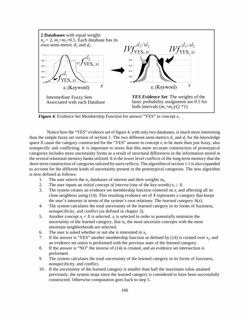
106

2 Databases with equal weight:nd = 2, m1=m2=0.5. Each database has itsown semi-metric d1 and d2.

YES Evidence Set: The weights of thebasic probability assignment are 0.5 forboth intervals (m1+m2)/(2 *1)

Intermediate Fuzzy SetsAssociated with each Database

Figure 4: Evidence Set Membership Function for answer “YES” to concept xi

Notice how the “YES” evidence set of figure 4, with only two databases, is much more interestingthan the simple fuzzy set version of section 1. The two different semi-metrics d1 and d3 for the knowledgespace X cause the category constructed for the “YES” answer to concept xi to be more than just fuzzy, alsononspecific and conflicting. It is important to stress that this more accurate construction of prototypicalcategories includes more uncertainty forms as a result of structural differences in the information stored inthe several relational memory banks utilized. It is the lower level conflicts of the long-term memory that theshort-term construction of categories tailored by users reflects. The algorithm of section 1.1 is also expandedto account for the different kinds of uncertainty present in the prototypical categories. The new algorithmis now defined as follows:

1. The user selects the nd databases of interest and their weights mk.2. The user inputs an initial concept of interest (one of the key-words) xi � X. 3. The system creates an evidence set membership function centered on xi and affecting all its

close neighbors using (14). This resulting evidence set of X represents a category that keepsthe user’s interests in terms of the system’s own relations: The learned category A(x).

4. The system calculates the total uncertainty of the learned category in its forms of fuzziness,nonspecificity, and conflict (as defined in chapter 3).

5. Another concept xj � X is selected. xj is selected in order to potentially minimize theuncertainty of the learned category, that is, the most uncertain concepts with the mostuncertain neighborhoods are selected.

6. The user is asked whether or not she is interested in xj.7. If the answer is “YES” another membership function as defined by (14) is created over xj, and

an evidence set union is performed with the previous state of the learned category. 8. If the answer is “NO” the inverse of (14) is created, and an evidence set intersection is

performed. 9. The system calculates the total uncertainty of the learned category in its forms of fuzziness,

nonspecificity, and conflict.10. If the uncertainty of the learned category is smaller than half the maximum value attained

previously, the system stops since the learned category is considered to have been successfullyconstructed. Otherwise computation goes back to step 5.

107

The algorithm can be supplemented with the inclusion of the uncertainty decreasing operation forevidence sets (as described in section 6 of chapter 3), in addition to the evidence set union and interaction.Often, the question-answering process might be lengthy, as the system tries to explore the uncertainty sourcesin the several databases. If the user decides to terminate the process to achieve a faster search, the uncertaintydecreasing operation can be used with pre-existing simple categories reflecting some often used queries. Suchcategories can be referred to as templates. When they are applied to the current knowledge space with theuncertainty-decreasing operation, the former is quickly simplified. This allows the system to escape a lengthyassociative process if a fast result is required. The details of this mechanism are not explored here since itdoes not affect the essentials of the algorithm and is not fundamental for understanding artificial categoryconstruction.

1.2.3 Document Retrieval

The mechanism of document retrieval is very similar to the one described in 1.1.3, except that theindices given by equations (5), (6) and (7) are adapted for evidence sets. First the evidence set category issimplified to its closest fuzzy set by a process of elimination of nonspecificity and conflict. Basically, thefuzzy membership is defined as the center of all weighted interval focal elements. Once this fuzzy set isobtained (5), (6), and (7) can be used.

1.2.4 Adaptive Alteration of Long-Term Structure

The adaptive alteration of the long-term structure is also essentially equivalent to the one describedin section 1.1.4. When concepts tend to be present in short-term learned categories, their relative distancein the long-term relational structure is adaptively reduced. The only difference is that now the long-termstructure is divided in several sub-databases. Thus, when two highly activated concepts in the learnedcategory are not present in the same database (each one exists in a different database) they are added to thedatabase which does not contain them, with property counts given by equations (8) and (9). If thesimultaneous activation keeps occurring, then a database that did not previously contain a certain concept,will have its presence progressively strengthened, even though such concept does not really possess anyproperties in this database – properties end up being associated with it through the concept’s relations tonative concepts of the database. This way, short-term memory not only adapts an existing structure to itsusers as the system in section 1.1, but effectively creates new elements in different, otherwise independent,relational databases, solely by virtue of its temporary construction of categories.

1.2.5 Categories as Linguistic, Metaphorical, Structural Perturbation

The evidence set question-answering system follows essentially the algorithm presented in section1.1 except that now the constructed categories capture more of the prototypical effects discussed in chapter3. Such “on the hoof” construction of categories triggered by interaction with users, allows several unrelatedrelational networks to be searched simultaneously, temporarily generating categories that are not really storedin any location. The short-term categories bridge together a number of possibly highly unrelated contexts,which in turn creates new associations in the individual databases that would never occur within their ownlimited context. Therefore, the construction of short-term linguistic categories in this artificial system,implements the sort of structural perturbation of a long-term system of associations discussed in chapter 2,section 2.4. It is in fact a system of recontextualization of otherwise, contextually constrained, independentrelational networks.

108

This transference of information across dissimilar contexts through short-term categorizationmodels some aspects of what metaphor offers to human cognition: the ability to discern correspondence innon-similar concepts [Holyoak and Thagard, 1995; Henry, 1995]. Consider the following example. Twodistinct databases are going to be searched using the system described above. One database contains thebooks of an institution devoted to the study of computational complex systems (e.g. the library of the SantaFe Institute), and the other the books of a Philosophy of Biology Department . I am interested in the conceptsof Genetics and Natural Selection. If I were to conduct this search a number of times, due to my owninterests, the learned category obtained would certainly contain other concepts such as AdaptiveComputation, Genetic Algorithms, etc. Let me assume that the concept of Genetic Algorithms does notinitially exist in the Philosophy of Biology library. After I conduct this search a number of times, the conceptof Genetic Algorithms is created in this library, even though it does not contain any books in this area.However, with my continuing to perform this search over and over again, the concept of Genetic Algorithmsbecomes highly associated with Genetics and Natural Selection, in a sense establishing a metaphor for theseconcepts. From this point on, users of the Philosophy of Biology library, by entering the keyword GeneticAlgorithms would have their own data retrieval system output books ranging from “The Origin of Species”to treatises on Neo-Darwinism – at which point they would probably bar me from using their networkeddatabase! The point is, that because of the Evidence Set system of short-term categorization that usesexisting, fairly contextually independent relational sub-networks, an ability to create correspondence betweensomewhat unrelated concepts is established.

1.2.6 Open-Ended Structural Perturbation

Given a large number of sub-networks comprised of context-specific associations, the categorizationsystem is able to create new categories that are not stored in any one location, changing the long-termmemory banks in an open-ended fashion. Thus the linguistic categorization Evidence Set mechanismachieves the desired system of open-ended structural perturbation of long-term networked memory. Asdiscussed in chapter 2, open-ended in terms of all the available dynamic building blocks that establish thepersonal construction of associations. Open-endedness does not mean that the categorizing system is ableto discern all physical details of its environment, but that it can permutate all the associative informationthat it constructs in an open-ended manner. Each independent network has the ability to associate newknowledge in its own context (e.g. as more books are added to the libraries of the prior examples): theseare the building blocks. To this, the categorization scheme adds the ability of open-ended associationsbuilt across contexts. Therefore, a linguistic categorization mechanism as defined above, offers theability to re-contextualize lower level dynamic memory banks, as a result of pragmatic, consensual,interaction with an environment. This linguistic consensual selection of dynamics, was identified inchapter 2 as the main idea behind Evolutionary Constructivism as the cognitive version of a theory ofembodied, evolving, semiosis.

1.2.7 TalkMine: The Implemented Application

An application named TalkMine was developed that implements the above specified system. It wasbuilt with the Delphi 2.0 application development environment for Windows 95. TalkMine accepts databasefiles from such standard databases such as Paradox and dbase. It is also equipped to deal with client-serverdatabases using SQL. The example shown below refers to a database of 150 of my own books. From the poolof 150 books three databases were created by randomly picking books from this pool with equal probability.Each sub-database is comprised of about 50 books, some of which exist in more than one of the sub-databases. Book records are the properties of the system described above. The fields created for these records

109

Figure 5: TalkMine with two Sub-Databases

were Title, Date, Authors, Publisher, plus 6 key-words describing the contents of the books. These keywordsare the concepts of the system described above. Naturally, many of these keywords overlap. From the 150books, 89 keywords were identified. Thus the system has 89 concepts and 150 properties. Figure 5 showsTalkMine’s first screen. Two databases are selected S3.DBD and S4.DBD.

After selecting two databases, the user selects the TalkMine ES option to mine the databases usingevidence sets (the TalkMine FS option uses Fuzzy Sets). The next screen shows the user all the conceptsTalkMine found in the sub-databases. The user can also set the � and � parameters introduced above,that specify how rough or precise the search is to be made and the membership threshold to preserveprevious answers. Figure 6 shows this screen.

110

Figure 6: Search Screen for TalkMine

Figure 7: Example of Question Posed by TalkMine

The user then selects an initial concept to start the search, in this case “ADAPTIVE SYSTEMS” ischosen. From this point on, the system starts the question-answering process described earlier, anexample of this interaction is shown in figure 7.

111

Figure 8: TalkMine’s Retrieval Screen

After a few steps, the system stops and a few data retrieval options are shown to the users (figure 8).Notice that, all concepts that received “YES” and “NO” answers are posited in their own respectiveboxes. Furthermore, a graphical interface showing the state of the (evidence set) knowledge space isdrawn throughout the question-answering process (figure 8).

Examples of retrieval results are shown in figures 9 and 10 for different retrieval options. Noticethat the options “Subsets”, “Whole”, and “Mix” refer to retrieval indices (5), (6), and (7) respectively. Figure11 shows another search this time for the concept “CATEGORIZATION”.

112

Figure 9: Results for “ADAPTIVECOMPUTATION” with R2=0.8

Figure 10: Results for “ADAPTIVECOMPUTATION” with R2=0.6

TalkMine implements the contextual construction ofshort-term categories from several long-term relationalstructures as described above. It is based on prototypicalcategories represented by evidence sets defined in Chapter 3.It is a reflection of the evolutionary constructivist positiondiscussed in chapter 2, as categories are constructed by thesystem’s own relational structure, which is in turnpragmatically adapted to the consensus of its users.

The long-term relational memory structureimplements the personal, subjective, aspects of cognitivesystems. It is this structure that ultimately dictates howcategories are constructed. The categories constructed areshort-term structures not stored in any location, butconstructed “on the hoof” as the system relates its severalrelational sub-networks to the interaction (conversation) usersprovide. Its syntax is based on evidence sets and theirextended theory of approximate reasoning. Semantics isestablished in accordance to the system’s internal relationalsemi-metrics, and how it pragmatically relates to the usersneeds.

TalkMine is therefore imbedded in the evolvingsemiotics framework also described in chapter 2.Furthermore, it explores contextual conflicting uncertaintyas a source of artificial category construction, since theselection of concepts for the question-answering process isbased on reducing the total uncertainty present in learnedcategories. Hence, TalkMine is a computational explorationof uncertainty, context, and subjectivity in cognitivesystems with very useful results for the field of data mining.It is an implementation of the ideas defendedphilosophically and mathematically in chapters 2 and 3.

113

Figure 11: Results for search on “CATEGORIZATION” withR1=0.6

37 Portions of the work here presented were published in Rocha [1997d]

114

F3 2x/L, x<L/2

22x/L, x�L/2

F5 0.25, x<L/20.75, x�L/2 F7

4x/L, x<L/41, x<3L/4

44x/L, x�3L/4

F9

0.52x/L, x<L/42x/L0.5, x<3L/45/22x/L, x�3L/4

F11 2x/L, x<L/2

2x/L1, x�L/2

F13

3x/2L, x<L/30.5, x<2L/33x/2L0.5, x�2L/3

F15 0.5x/L, x<L/2x/L, x�L/2

2. Emergent Morphology and Evolving Solutions in Large State Spaces37

The Contextual Genetic Algorithm (CGA) with fuzzy indirect encoding defined by FuzzyDevelopment Programs (FDP’S) described in chapter 4 (section 5.2), was applied to two different cases. Thefirst one refers to the evolution of weights for a large neural network; it is a continuous variable problem.The second, refers to the evolution of Cellular Automata (CA) rules for solving non-trivial problems; it isa discrete variable problem.

2.1 Implementation Details

Both problems were approached with the same FDP architecture. 16 fuzzy set shapes are definedin pool ) (nF = 16), specified by the following functions defined for x � [0, L]:

F1 = x/L F2 = 1-F1 F4 = 1-F3

F6 = 1-F5

F8 = 1-F8

F10 = 1-F9

F12 = 1-F11

F14 = 1-F13

F16 = 1-F15

16 fuzzy set operations are defined in pool 2�(nO = 16): X1 = F, X2 = �, X3 = Avg, X3 = Avg, X4 =1 - Avg, X5 = , X6 = , X7 = , X8 = , X9 = , X10 = , X11 = A.B, X12 = 1 - A.B,ABB AAB ABB AAB ABB AAB

X13 = , X14 = , X15 = , and X16 = . All these operations are simple linearAB (A#B) AA (A#B) BB (A#B) BA (A#B)functions of two generic fuzzy sets A and B.

38 These patterns were obtained from Don Gause with his permission from the data files of theNeural Network and Genetic models class.

115

The universal set X of the problems presented next was divided in 16 Parts (nX = 16). Someexperiments were also conducted with nX = 32 which will be identified ahead. Experiments were conductedwith FDP’s of lengths n = 8, 16, and 24, which according to equation (1) in chapter 4, section 5.2.3, requirebinary chromosomes of lengths � = 144, 288, and 432 respectively.

2.2 Continuous Variables: Evolution of Neural Network Weights

Interesting results have been obtained when using genetic algorithms (GA’s) to evolve the weightsof a neural network with a fixed architecture. For instance, Montana and Davis [1989] utilized a GA insteadof a standard training algorithm such as back-propagation to find a good set of weights for a givenarchitecture. It is reasoned that the advantage of using GA’s instead of back-propagation lies in the latter’stendency to get stuck at local optima, or the unavailability of a large enough set of training patterns forcertain tasks [Mitchell, 1996a]. I explore the problem here, not to prove or disprove its merits, but simplybecause it is usually a very computationally demanding problem, which can potentially benefit from thechromosomal information compression offered by CGA’s with fuzzy indirect encoding.

The set of weights of a neural network defines a vector of real values. Montana and Davis’ networkrequired a vector of 126 weights to evolve. Because the weights are real-valued, they used what is usuallyreferred to as the real encoding of chromosomes in a GA. That is, instead a binary strings as chromosomes,a real-encoded GA uses strings of real numbers. The operation of mutation is now different: a randomnumber is added to each element of the vector with low probability. Montana and Davis also used a differentkind of crossover operation, the details of which are unnecessary for the current presentation (see Montanaand Davis [1989] for more details).

2.2.1 Hand-Written Character Recognition: The Network Architecture

I applied the CGA with fuzzy indirect encoding to a problem that requires larger real-valuedchromosome vectors. The problem I approached was that of the recognition of hand-written characters in an8 by 10 grid38: each pattern is defined by an 80 bits long vector. There were a total of 260 patterns available,which contained 5 different categories, that is 5 different hand-written characters with 52 instance patternseach. The patterns were divided equally between the learning and the validation sets, preserving the ratiosper category. In other words, the learning and the validation sets contained both 130 patterns, 26 patterns foreach of the 5 categories.

Since each pattern is an 80-length bit vector, the input layer to the neural network has also 80nodes, plus one for the bias unit. The output layer requires only 3 nodes, whose binary output encode 5categories (3 nodes can encode up to 8 categories). Experiments were ran with a hidden layer of 2 and 5Nodes. The information requirements of the sets of weights for these architectures are summarized in thefollowing table:

116

Figure 12: Typical run for back-propagation network with 2 hidden nodes

Neural Network Architecture with 81 input nodes and 3output nodes

Hidden Nodes 2 5

Number of Weights 171 423

Bits of Information (4 byte real number)

5472 13536

Thus, the real encoded GA requires chromosomes defined by real-valued vectors of length 171 and423, for the 2 and 5 hidden nodes architectures, respectively. Such vectors actually cost some computerimplementation 5472 and 13536 bits of information each (assuming an implementation where real numbersare only 4 bytes long which is actually rather small).

2.2.2 Results from Back-Propagation

The results reached by the back-propagation algorithm are irrelevant to establish CGA’s with fuzzyindirect encoding, since the results from these are to be compared instead with traditional GA’s. In any case,for this problem, back-propagation classified the patterns much better than either GA, and can be regardedas an upper limit for the desired behavior of classifying systems. A typical run is shown in figure 12. Thenetwork converges easily to the 130 patterns of the learning set. The number of correctly classified patternsin the validation set does not surpass 100 patterns. Networks with more hidden nodes converge a bit faster

to the learning set, but do not result in better classifications of the validation set. 100 runs were performed,50 for each architecture. The learning set converged every time, while the average cross-validation was closeto 94 patterns out of 130. The following table summarizes the results.

39 Other values of these probabilities were tried, as well as other fitness functions. The set ofparameters described above proved to be the most efficient.

117

Figure 13: Typical weight vector for back-propagation network with 2 hiddennodes.

Back-Propagation Algorithm

Number of Hidden Nodes 2 5

Number of Runs 50 50

Average number of correctly classifiedpatterns in learning set

130 130

Average number of correctly classifiedpatterns in validation set

93.2 94.4

A typical weight vector obtained from the state of the network whose run is depicted in figure 12when highest cross-validation was reached, is shown in figure 13.

2.2.3 Results from Real-encoded GA

The runs with a standard GA were performed with real-encoded chromosomes (the weight vectors).The population size was set to 100 elements. Each run consisted of 500 generations. The fitness function wasdefined simply as the number of correct classifications of the patterns in the learning set. In each generation,every chromosome was decoded into a network and the learning set presented to it. The network weightvectors that classified more patterns had higher probability of selection into the next generation. Probabilityof crossover was set to 0.7, and probability of mutation to 0,00239. The following table presents the resultsobtained.

118

Figure 14: Weight Vector for Network with 2 hidden nodes obtained with GA

Real-Encoded GA

Number of Hidden Nodes 2 5

Number of Runs 50 50

Average Time of runs (min) 7 24

Average number of correctly classifiedpatterns in learning set

108.7 114.7

Average number of correctly classifiedpatterns in validation set

81.8 79.9

The average time of runs refers to the particular computational setup I used: an Intel Pentium166MHz. The code was written using Delphi 2.0. This algorithm is very computationally demanding due toextensive floating point operations, since the weight vectors are real-valued. The average time for each runincreases dramatically with the number of hidden nodes included. The algorithm never converges completelyto the learning set, but does reach comparable, though lower, results to the back-propagation algorithm forthe validation patterns. Notice that the network with 5 hidden nodes did not yield as good results forvalidation as the one with 2 hidden nodes, though the reverse happened for the learning set. Figure 14 showsa typical weight vector obtained by the GA for a network with two hidden nodes. Notice that it is more

random that the one obtained from back-propagation. I believe that this more random pattern causes thenetwork to overly adapt to the learning set and fail to generalize the categorical relationships properly. Thismight explain why networks with more hidden nodes present worse cross-validation behavior, since theweight vector that overly adapted to the specific relationships of the learning set is much larger, and beingvery random, the probability that it will also categorize the validation set will be smaller.

119

2.2.4 Results from CGA with Fuzzy Indirect Encoding

The fuzzy indirect encoding of the networks’ weight vectors, transforms them from real-valuedvectors to binary vectors represented by FDP’s. That is, the CGA uses as chromosomes not the weightvectors directly, but binary FDP’s that indirectly encode weight vectors. The length of the binary FDP’s isin bits presented in the following table according to the parameters specified in section 2.1. The length inbits is calculated with equation (1) defined in chapter 4, section 5.2.3.

FDP Length (n) 8 16 24

16 Partitions (nX=16) 144 288 432

32 Partitions (nX=32) 168 336 504

Compare the bit sizes of these chromosomes to the ones required of real-encoded chromosomesas shown in the table in section 2.2.1. For instance, to encode a 5 hidden nodes network with direct real-valued chromosomes we need 13536 bits, while with fuzzy indirect encoding we only need 144 to 504 bitsdepending on the parameters of the FDP. Notice that the size of the FDP is not dependent on the size of thenetwork. From the point of view of the chromosomes, it is the same to encode a 2 or 5 hidden layer network.However, though the chromosomes do not depend on the size of the network, the fitness evaluation naturallydoes. Indeed, each chromosome will be decoded into a specific network that is eventually evaluated regardingthe problem at stake. Indirect encoding can only off-load computational effort from the encoding andvariation portions of GA’s, not from the evaluation steps. The results from the indirect encoding runs areshown on the following tables:

Fuzzy Indirect Encoding CGA with nX=16

Hidden Nodes 2 5

FDP Length 8 16 24 8 16 24

Number of runs 50 50 50 35 50 20

Avg. Run time (min) 3 3 3 15 16 17

Avg. Correct Patternsin Learning Set

95.0 98.2 107 92.2 98.3 96

Avg. Correct Patternsin Validation Set

80.1 81.6 82.9 77.5 84.1 77.5

120

Fuzzy Indirect Encoding CGA with nX=32

Hidden Nodes 2 5

FDP Length 8 16 24 8 16 24

Number of runs 20 20 - - 20 -

Avg. Run time (min) 3 4 - - 18 -

Avg. Correct Patternsin Learning Set

98.2 96.1 - - 96.6 -

Avg. Correct Patternsin Validation Set

79.8 78 - - 80.3 -

The first thing to observe from these tables is that there was no advantage in increasing the numberof partitions of the universal set of the FDP’s. Even though a considerable smaller number of experimentswas conducted for 32 partitions, the results were generally worse than the experiments with 16 partitions.The results from the 16 partitions cases were, however, very promising. The indirect encoding runs took asluttle as half the time as the direct encoding ones with comparable results. The standard GA showed betterresults for the patterns in the learning set, however, better cross validation results were obtained on averageby the fuzzy indirect encoding scheme. For the 2 hidden nodes network, the highest average of correctpatterns in the validation set was obtained by the CGA with fuzzy indirect encoding with FDP’s with 24fuzzy sets (82.9), slightly better than the cross-validation obtained by the regular GA (81.8). For the 5 hiddennodes network, the difference was even higher: 84.1 for the CGA, and 79.8 for the GA.

Notice that the objective was not to top GA’s, but simply to obtain comparable results. The indirectencoding scheme reduced the chromosome size dramatically. Consequently, the computation time wasstrongly cut down, not just because of the size of chromosomes was strongly reduced but because insteadof floating-point operations the genetic operations are now based on boolean variables. FDP’s work byconstructing simple linear functions (the fuzzy set shapes in section 2.1) over the solution space (the weightvector in this case). Therefore, it restricts solutions into the reduced space of possibilities built out of simplelinear functions.

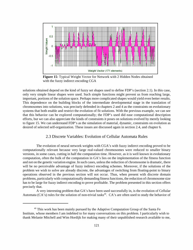
This reduction is apparent in Figure 15 that shows a typical weight space obtained by the CGA fora network with 2 hidden nodes. Indeed, the weight vector is not random, we can detect the simple fuzzy setshapes used by the FDP’s repeated here an there. It is obvious that this scheme tries to explore non-randomrelationships in the solutions reached, whereas the traditional GA reaches much more random solutions. Itis remarkable that the sort of ordered solutions reached by the CGA with fuzzy indirect encoding are actuallygood solutions. It shows that the problem being approached is rich in simple relationships that can beexplored. This might explain why the CGA obtained better results for cross-validation than the traditionalGA. The latter seems to converge well to specific solutions that solve the particular patterns in the validationset, but it is not as good at generalizing the categorical relationships in the data needed for good cross-validation results.

We can also observe that the indirect encoding scheme introduces a number of parameters that mayend up dictating its behavior. For instance, FDP’s of length 16 encoding networks with 5 hidden nodes,seemed to work better for this problem than all others. Moreover, and more importantly, ultimately the

40 This work has been mainly pursued by the Adaptive Computation Group of the Santa FeInstitute, whose members I am indebted to for many conversations on this problem. I particularly wish tothank Melanie Mitchell and Wim Hordijk for making many of their unpublished research available to me,

121

Figure 15: Typical Weight Vector for Network with 2 Hidden Nodes obtainedwith the fuzzy indirect encoding CGA

solutions obtained depend on the kind of fuzzy set shapes used to define FDP’s (section 2.1). In this case,only very simple linear shapes were used. Such simple functions might prevent us from reaching large,important, portions of the solution space. Perhaps more complicated shapes would yield even better results.This dependence on the building blocks of the intermediate developmental stage in the translation ofchromosomes into solutions, was precisely defended in chapters 2 and 4 as the constraints on evolutionarysystems that both enable and restrict the evolution of fit solutions. With the previous example, we can seethat this behavior can be explored computationally; the FDP’s used did ease computational descriptionefforts, but we can also appreciate the kinds of constraints it poses on solutions evolved by merely lookingto figure 15. We can understand FDP’s as the simulation of material, dynamic, constraints on evolution asdesired of selected self-organization. These issues are discussed again in section 2.4, and chapter 6.

2.3 Discrete Variables: Evolution of Cellular Automata Rules

The evolution of neural network weights with CGA’s with fuzzy indirect encoding proved to becomputationally relevant because very large real-valued chromosomes were reduced to smaller binaryversions, in some cases, cutting in half the computation time. However, as it is well known in evolutionarycomputation, often the bulk of the computation in GA’s lies on the implementation of the fitness functionand not on the genetic variation engine. In such cases, unless the reduction of chromosome is dramatic, therewill be no perceivable advantage of fuzzy indirect encoding schemes. Moreover, if the solutions of theproblem we wish to solve are already discrete, the advantages of switching from floating-point to binaryoperations observed in the previous section will not occur. Thus, when present with discrete domainproblems, particularly with computationally demanding fitness functions, the reduction of chromosome sizehas to be large for fuzzy indirect encoding to prove profitable. The problem presented in this section offersprecisely that.

A very interesting problem that GA’s have been used successfully in, is the evolution of CellularAutomata (CA’s) rules for the solution of non-trivial tasks40. CA’s are often used to study the behavior of

without which I would not be able tackle the problem.

122

Figure 16: Space-time diagram of one-dimensional CA’s as theydeal with the density task.

complex systems, since they capture the richness of self-organizing dynamical systems which from localrules amongst their components, observe emergent behavior (see chapter 2). “CAs are decentralized spatiallyextended systems consisting of a large number of simple identical components with local connectivity.”[Mitchell, 1996b, page 1].The components (cells) are finite-state machines arranged in a lattice N, each withan identical state transition rule based upon the state of their immediate neighbors. The CA’s used in thissection are one-dimensional with binary states.

Certain CA rules are capable of solving global tasks assigned to their lattices, even though theirtransition rules are local. One such tasks is usually referred to as the density task: given a randomly initializedlattice configuration, the CA should converge to a global state where all its cells are turned “ON” if there isa majority of “ON” cells in the initial configuration (IC’s), and to an all “OFF” state otherwise. This rule isnot trivial precisely because the local rules of the component cells do not have access to the entire lattice,but can only act on the state of their immediate neighborhood. Crutchfield and Mitchell [1995] used a GAto evolve the CA rules for such a task. They used one-dimensional CA’s with 149 cells. The local rule of thisCA works on a neighborhood of 7 cells (the rule’s cell plus 3 cells to each side), which is often referred toas a neighborhood of radius 3. Such a rule has 128 possible states since the CA is binary (27=128), and soit is defined by a lookup table with 128 entries. To encode such a lookup table in a GA we require only a128-bit string if we fix the order of the lookup table entries. Their GA used a population of 100 of suchrandomly initialized GA’s. The fitness of each rule was computed by iterating the corresponding CA on 100randomly chosen ICs uniformly distributed over the density of “ON” cells, '0 � [0, 1], half with '0 < 0.5(correct classification all “OFF’s”) and half with '0 > 0.5 (correct classification all “ON’s”), and byrecording the fraction of correct classifications performed in a certain number of steps (usually a bit over 2N)[Ibid, page 10743]. Notice how computationally demanding this fitness function is, as every singlechromosome has to be decoded into a CA and run for about 300 cycles.

The GA found a number of fairly interesting rules, but 7 out of the 300 runs evolved veryinteresting rules (with high fitness) which create an intricate system of lattice communication. Basically,groups of adjacent cells propagate certain patterns across the lattice, which as they interact with other suchpatterns “decide” on the appropriate solutions for the lattice as a whole. Several types of signaling patternsand their communication syntax have been identified, and can be said to observe the emergence of

41 This fitness is not the same as the one used in the GA. The latter uses IC’s whose density ofON’s is uniformly distributed in the unit interval, while the former is the so-called unbiased fitness. It iscomputed by randomly flipping each bit of the IC’s with equal probability. This results in densities closerto 0.5 which are the toughest for the rule to tackle.

123

Figure 17: Typical CA rule of radius 3 evolved with the traditional GA.Each element of the horizontal axis represents an entry of the rule’slookup table. A bar denotes an “ON” state. The hexadecimalrepresentation of the 128-bit string this rule defines is:8000C0400010216FEFC9EFFDFFEFFEEF

embedded-particle computation in evolved CA’s [Ibid; Hordijk, Crutchfield, Mitchell, 1996]. Figure 16(from [Crutchfield and Mitchell, 1995] shows 2 examples of these rules as they tackle the same IC, the firstrule (a) classifies the IC properly while the second (b) misclassifies. The space-time diagram shows thetemporal development of the one-dimensional lattice. Each line represents the state of the lattice at aparticular instance. Black cells are “ON” states, while white cells are “OFF” states. Notice the existence ofseveral types of areas, which define the signaling particles. The best rules for this system have a fitness of0.74, while the average fitness for all rules evolved by their GA was 0.6441.

I replicated their experiments and obtained the same value for average fitness, but the rule withhighest fitness I encountered rated only 0.67. This may have been because, due to very lengthy computations,I only tried 75 runs (they found only 7 particle-computation rules out of 300 runs). In any case, my aim wasto apply the fuzzy indirect encoding scheme to this problem, so the bulk of my effort was pursuing this aimand not to replicate their experiments. I used the CGA with fuzzy indirect encoding with the parametersdescribed in section 2.1, with FDP’s of length 8 and 16, which require binary chromosomes of length 144and 288 respectively. Since their chromosomes use 128 bit-strings, there is no advantage in using fuzzyindirect encoding for this problem, except that it is important to compare the results. 120 runs wereperformed and the same average fitness 0.64 was obtained. The maximum fitness I observed was once again0.67. In other words, I obtained the same results with the CGA than with my runs of the regular GA.

I never evolved one of the particle-computation rules for CA’s with neighborhoods of radius 3. Atleast in my experiments, there was no difference between the performances of the directly and indirectly

encoded GA’s. Figures 17 and 18 show the highest rules evolved for the two cases. Both are similar and quitetypical of the rules evolved: the lookup entries towards the end of the binary vector tend to be “ON”, whilethe ones on the left ten to be “OFF”. This is natural since the first (last) elements in the lookup table refer

124

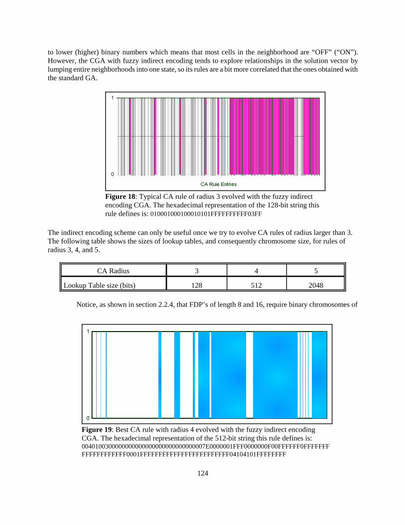
Figure 18: Typical CA rule of radius 3 evolved with the fuzzy indirectencoding CGA. The hexadecimal representation of the 128-bit string thisrule defines is: 010001000100010101FFFFFFFFFF03FF

Figure 19: Best CA rule with radius 4 evolved with the fuzzy indirect encodingCGA. The hexadecimal representation of the 512-bit string this rule defines is:0040100300000000000000000000000000007E0000001FFF0000000F00FFFFFF0FFFFFFFFFFFFFFFFFFF0001FFFFFFFFFFFFFFFFFFFFFFFF04104101FFFFFFFF

to lower (higher) binary numbers which means that most cells in the neighborhood are “OFF” (“ON”).However, the CGA with fuzzy indirect encoding tends to explore relationships in the solution vector bylumping entire neighborhoods into one state, so its rules are a bit more correlated that the ones obtained withthe standard GA.

The indirect encoding scheme can only be useful once we try to evolve CA rules of radius larger than 3.The following table shows the sizes of lookup tables, and consequently chromosome size, for rules ofradius 3, 4, and 5.

CA Radius 3 4 5

Lookup Table size (bits) 128 512 2048

Notice, as shown in section 2.2.4, that FDP’s of length 8 and 16, require binary chromosomes of

125

Figure 20: Space-time diagram of bestCA rule of radius 4

Figure 21: Space-Time View of the Bestrule evolved for a CA rule of radius 4

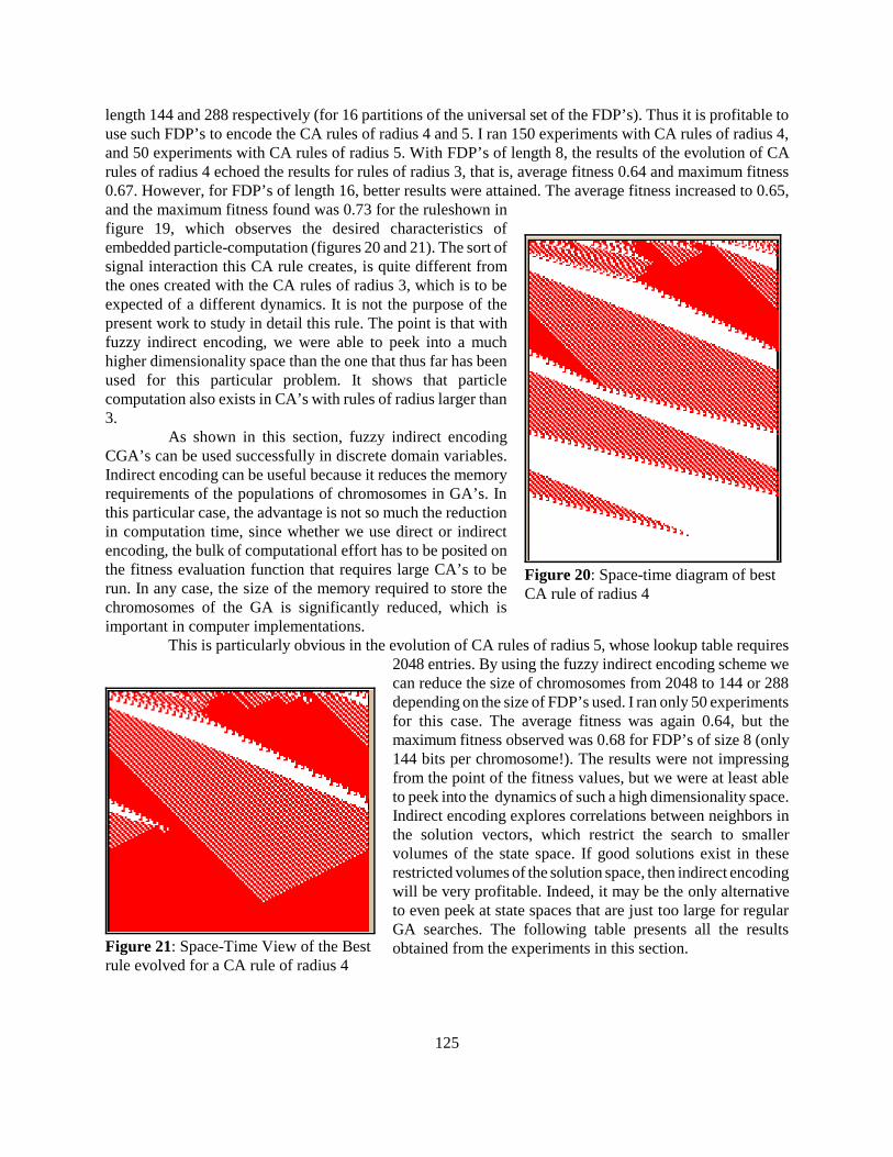
length 144 and 288 respectively (for 16 partitions of the universal set of the FDP’s). Thus it is profitable touse such FDP’s to encode the CA rules of radius 4 and 5. I ran 150 experiments with CA rules of radius 4,and 50 experiments with CA rules of radius 5. With FDP’s of length 8, the results of the evolution of CArules of radius 4 echoed the results for rules of radius 3, that is, average fitness 0.64 and maximum fitness0.67. However, for FDP’s of length 16, better results were attained. The average fitness increased to 0.65,and the maximum fitness found was 0.73 for the ruleshown infigure 19, which observes the desired characteristics ofembedded particle-computation (figures 20 and 21). The sort ofsignal interaction this CA rule creates, is quite different fromthe ones created with the CA rules of radius 3, which is to beexpected of a different dynamics. It is not the purpose of thepresent work to study in detail this rule. The point is that withfuzzy indirect encoding, we were able to peek into a muchhigher dimensionality space than the one that thus far has beenused for this particular problem. It shows that particlecomputation also exists in CA’s with rules of radius larger than3.

As shown in this section, fuzzy indirect encodingCGA’s can be used successfully in discrete domain variables.Indirect encoding can be useful because it reduces the memoryrequirements of the populations of chromosomes in GA’s. Inthis particular case, the advantage is not so much the reductionin computation time, since whether we use direct or indirectencoding, the bulk of computational effort has to be posited onthe fitness evaluation function that requires large CA’s to berun. In any case, the size of the memory required to store thechromosomes of the GA is significantly reduced, which isimportant in computer implementations.

This is particularly obvious in the evolution of CA rules of radius 5, whose lookup table requires2048 entries. By using the fuzzy indirect encoding scheme wecan reduce the size of chromosomes from 2048 to 144 or 288depending on the size of FDP’s used. I ran only 50 experimentsfor this case. The average fitness was again 0.64, but themaximum fitness observed was 0.68 for FDP’s of size 8 (only144 bits per chromosome!). The results were not impressingfrom the point of the fitness values, but we were at least ableto peek into the dynamics of such a high dimensionality space.Indirect encoding explores correlations between neighbors inthe solution vectors, which restrict the search to smallervolumes of the state space. If good solutions exist in theserestricted volumes of the solution space, then indirect encodingwill be very profitable. Indeed, it may be the only alternativeto even peek at state spaces that are just too large for regularGA searches. The following table presents all the resultsobtained from the experiments in this section.

126

Regular GA Fuzzy Indirect Encoding CGA

CA Rule Radius 3 3 4 5

Number of Runs 75 120 150 50

Average Fitness 0.64 0.64 0.64(n=8)

0.65(n=16)

0.64(n=8)

0.64(n=16)

Best Fitness 0.67 0.67 0.67(n=8)

0.73(n=16)

0.68(n=8)

0.67(n=16)

2.4 The Effectiveness of Computational Embodiment: Epistasis and Development

The introduction of an intermediate development layer in CGA’s serves to reduce the size ofgenetic descriptions (see chapter 4). This is done because some fixed computationally building blocks areassumed for any problem we encode. Chromosomes code for these building blocks which will themselvesself-organize (develop) into a final configuration. The algorithm used in this chapter achieves precisely that.It is an instance of the selected self-organization ideas presented in chapter 2. The developmental stage isin effect simulating some specific dynamic constraints on evolution posed by a simulated embodiment of theevolving semiotic system.

Fuzzy indirect encoding captures computationally the advantages of materiality by reducing geneticdescriptions, which may be very relevant in practical domains such as data mining. However, it does alsocapture the reverse side of embodiment, that is the limiting constraints that a given materiality poses onevolving systems. Given a specific simulated embodiment defined by the particular fuzzy set shapes andoperations used (see section 2.1), the algorithm cannot reach all portions of space of solutions. It can onlyreach those solutions that can be constructed from the manipulation of the allowed fuzzy sets and operations– the building blocks. This echoes my early observation (see chapter 2 and 4), that the genetic system issimilarly not able to evolve anything whatsoever, but only forms that can be built out of aminoacid chains.Such constraints are observed on the problems of sections 2.2 and 2.3, as the solution vectors obtained bythe indirect encoding scheme are much less random than the solutions obtained by direct encoding. Thesolutions reached are much more ordered, in other words, the inclusion of the developmental stage introduceda lot of order “for free”. Such order was not a result of the selection mechanism, but of the intrinsic dynamicsthe system possesses (the developmental rules) that tends to produce mostly ordered solutions.

Another way to think of this, is that in traditional GA’s, each position of the solution vector mapsto only one position in the chromosomes (allele), which can be independently mutated. In other words, themutation of one bit in the chromosome will affect only one component in the solution vector. Whereas in theindirect encoding scheme, each bit of the chromosomes affects several elements of the solution vector non-linearly. In the scheme here utilized, flipping one bit in the FDP may result in changing a fuzzy set operationto another, thus causing the fuzzy sets it operates on to be connected in a totally different manner for all itselements. Thus, one single bit of indirectly encoded chromosomes can affect many, potentially all, elementsof the solution vector as the development program is changed. This introduces epistasis to evolutionarycomputation, which we know exists in natural genetic systems.

All of these aspects of indirectly encoded GA’s, both enabling constraints such as geneticinformation compression, and limiting constraints such as reduction of the space of solutions, are desired ofmodels of evolutionary systems. But what does it mean for practical applications in data mining? Geneticcompression is obviously a plus, but the limiting constraints may be problematic if the reduced search spaceincludes only mediocre solutions to our problems. When genetic descriptions are not very large, the only

127

reason to use indirect encoding is if we wish to avoid very random solution vectors that tend to be producedwith GA’s. This was the case of the evolution of neural network weights in section 2.2. The indirect encodingscheme was able to produce better cross-validation results. Due to its intrinsic order, its solutions did notoverly adapt to the patterns in the learning set. When the genetic descriptions are very large, or require real-encoding (such as the case of section 2.2), then it is advantageous to use indirect encoding. Sometimes, evenif the reduced solution space is mediocre, such less that optimum solutions might be all that we can hope tofind in huge solution spaces, inaccessible to standard GA’s due to computational limitations.