Embed Size (px)
Citation preview

Chapter 5
Coarse circuit switching in the core
5.1 Introduction
In Chapters 1, 2 and 3, we have seen how we can benefit from having more cir-
cuit switching in the core of the Internet; circuit switching allows us to build switches
with fast all-optical data paths. Moreover, circuit switching can provide higher capac-
ity and reliability than packet switching without degrading end-user response time.
Chapter 4 described TCP Switching, an evolutionary way of integrating a circuit-
switched backbone with the rest of the Internet. This integration of circuit and
packet switching was done by mapping application flows to fine-grain, lightweight
circuits.
One problem of TCP Switching is that currently most crossconnects in circuit
switches cannot switch at the 56-Kbit/s granularity that was proposed in Chapter 4.1
It would be extremely wasteful to reserve an STS-1 channel or a wavelength exclu-
sively for a single user flow whose peak rate is limited to only 56 Kbit/s by its access
link. Another shortcoming, caused by several crossconnect technologies and signaling
mechanisms in circuit switching, is that it may take tens or hundreds of millisec-
onds to reconfigure the switch or to exchange the signaling messages that create a
new circuit. These long circuit-creation latencies occur when the crossconnect has to
1Typically, electronic SONET circuit switches use circuit granularities of STS-1 (51 Mbit/s) orhigher, whereas DWDM switches have granularities of OC-48 (2.5 Gbit/s) or higher.
95

96 CHAPTER 5. COARSE CIRCUIT SWITCHING IN THE CORE
move electromechanical parts, such as MEMS mirrors, or when the signaling requires
a positive acknowledgement from the egress circuit switch.
This chapter addresses these two limitations of circuit-switching technologies.
More precisely, it explores ways of using circuit switching in the Internet when cross-
connects have granularities that are much larger than the peak rate of user flows, and
when circuit switches are slow to reconfigure.
In this chapter, I propose monitoring the bandwidth that is carried by all user flows
between each pair of boundary routers around a circuit-switched cloud in the core.
This measurement provides an anticipating and stable estimation of the traffic matrix
that is then used to properly size the coarse-granularity circuits that interconnects
the boundary routers. In order to compensate for the circuit-creation latency of the
network, I propose allocating these circuits using an additional safeguard band that
prevents the circuits from overflowing.
One of the themes developed in Chapter 4 is again the basis for this chapter;
namely, how one can configure the circuit-switched backbone by monitoring the ac-
tivity of user flows. The difference is that now a core circuit is carrying many user
flows simultaneously, and so the mapping between user flows and circuits is not as
straightforward as that discussed in Chapter 4. It is no longer a matter of when to
create the circuits but how much capacity to assign to them.
5.1.1 Organization of the chapter
Section 5.2 defines the problem addressed in this chapter and describes other ap-
proaches that have been proposed by other researchers. Section 5.3 shows how one
can control a circuit-switched Internet core by monitoring user flows. Section 5.4
builds a model for the buildup of user flows. Then, Section 5.5 discusses some of the
implications of this approach. Finally, Section 5.6 concludes this chapter.
5.2. BACKGROUND AND PREVIOUS WORK 97
Circuit-
switched
cloud
Core
circuit
switchesBoundary
routers
Regular
routers
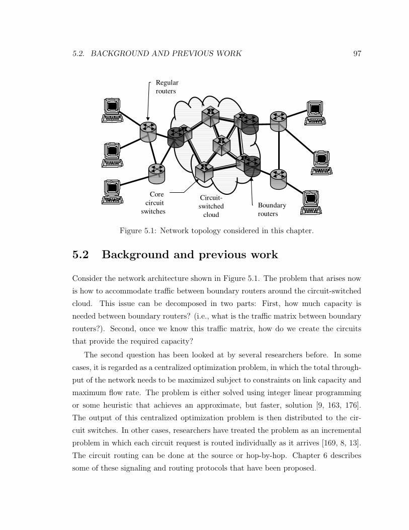
Figure 5.1: Network topology considered in this chapter.
5.2 Background and previous work
Consider the network architecture shown in Figure 5.1. The problem that arises now
is how to accommodate traffic between boundary routers around the circuit-switched
cloud. This issue can be decomposed in two parts: First, how much capacity is
needed between boundary routers? (i.e., what is the traffic matrix between boundary
routers?). Second, once we know this traffic matrix, how do we create the circuits
that provide the required capacity?
The second question has been looked at by several researchers before. In some
cases, it is regarded as a centralized optimization problem, in which the total through-
put of the network needs to be maximized subject to constraints on link capacity and
maximum flow rate. The problem is either solved using integer linear programming
or some heuristic that achieves an approximate, but faster, solution [9, 163, 176].
The output of this centralized optimization problem is then distributed to the cir-
cuit switches. In other cases, researchers have treated the problem as an incremental
problem in which each circuit request is routed individually as it arrives [169, 8, 13].
The circuit routing can be done at the source or hop-by-hop. Chapter 6 describes
some of these signaling and routing protocols that have been proposed.

98 CHAPTER 5. COARSE CIRCUIT SWITCHING IN THE CORE
(a)
(b)
(c)
Figure 5.2: Daily (a), weekly (b) and monthly (c) average traffic traces in a 1-Gbit/sEthernet link between Purdue University and the Indiana GigaPoP connecting toInternet-2 [63], as observed on February 5th, 2003. The dark line indicates outgoingtraffic; the shaded area indicates incoming traffic. The low traffic in weeks 0 and 1in graph (c) corresponds to the last week of December 2002 and the first week ofJanuary 2003, respectively, when the university was in recess.
This chapter focuses on the first question, how to estimate the traffic matrix
between boundary routers and then use the estimate to provision coarse-granularity
circuits. Some researchers [9, 163, 120] have suggested that future traffic matrices can
be predicted off-line using past observations. These researchers point out that traffic
in the core of the network is smoother than at the edges and that it follows strong
hourly and daily patterns that are easy to characterize, as shown in Figure 5.2. For
example, traffic is affected by human activity and scheduled tasks, and so peak traffic
occurs during work hours on weekdays, whereas at night and during weekends there
is less traffic.
Nonetheless, this off-line prediction of the traffic matrix fails to forecast sudden

5.2. BACKGROUND AND PREVIOUS WORK 99
changes in traffic due to external events, such as breaking news that creates flash
crowds, a fiber cut that diverts traffic or the new version of a popular program that
generates many downloads. Only an on-line estimation of the traffic matrix would be
able to accommodate these sudden and unpredictable changes in traffic patterns.
This on-line estimation of traffic could be done in several ways. One of them is
to monitor the aggregate packet traffic [79], either by observing the instantaneous
link bandwidth or the queue sizes in the routers. While this approach does not
require much hardware support and is easy to implement, it does not provide good
information about the traffic trends. Packet arrivals present many short- and long-
range dependencies that make both the instantaneous arrival rates and queue sizes
fluctuate wildly. In contrast, I propose using another way of estimating the current
traffic usage by monitoring user flows. It requires more hardware support, but, in
exchange, user flows provide a traffic estimation that is more predictive and has less
variation, at least for the circuit-creation latencies under consideration (1ms-1 s), as
we will see below.
Figure 5.3 gives a clear example of the fluctuations in the instantaneous arrival
rate. The dots in the background denote the instantaneous link bandwidth over 1-ms
time intervals. With so much noise, it is difficult to see any trends in the data rates.
Thus, one could apply filters to smooth the signal. For example, the dark gray line
in Figure 5.3 shows the moving average R(t) = (1 − α)R(t − ∆t) + αr(t), where r(t)
is the instantaneous measure, ∆t is 1ms and α is 0.10. The figure also shows the
instantaneous traffic rate over 100-ms intervals (light gray line) and the sum of the
average bandwidth of the active flows (black line). The average bandwidth of a flow is
the total number of bits that are transmitted divided by the flow duration. Of course,
the flow average bandwidth is something that is not known when a flow starts, but
I will explain below how to estimate an upper bound in the next section. One can
see that the 100-ms bin size provides the signal with the least noise of all measures of
traffic based on counting packets, but there are still many more fluctuations than in
the measure based on the average bandwidth of active flows, from which the trends
are much clearer. In brief, user flows provide more stable measurement than packets
and queue sizes for time scales between 1ms and 1 s.

100 CHAPTER 5. COARSE CIRCUIT SWITCHING IN THE CORE
Figure 5.3: Time diagram showing the instantaneous link bandwidth over 1-ms inter-vals (dots), its time moving average (dark gray line), the instantaneous link bandwidthover 100-ms intervals (light gray line) and the sum of the average rate of all activeflows (black line). The trace was taken from an OC-12 link on January 18th, 2003[131].
User flows also provide an advance notice before major changes in bandwidth
utilization occur. For example, we can see that in Figure 5.3 there is a sudden
increase in traffic between times 21 s and 46 s (due to a single user flow whose only
constraint was a 10-Mbit/s link). This traffic increase was predicted four seconds
before it happened by observing the active flows. There are two reasons for this
advance notice: first, an application may take some time to start sending data at
full rate after it connected with its peer.2 Second, it takes several round-trip times
for TCP connections to ramp up their rate to the available throughput because of
the slow-start mechanism. In contrast, when we monitor the instantaneous arrival
2This is the main reason for the advance notice in Figure 5.3. Unfortunately, it was impossibleto know what application caused this behavior because the trace was “sanitized”.

5.3. MONITORING USER FLOWS 101
rate to estimate the traffic matrix, the filters that are applied to reduce the noise
add some delay to the decision making of whether more capacity is needed. If the
circuit creation mechanism already takes a long time, adding more delay in the traffic
estimation makes the system react more slowly.
5.3 Monitoring user flows
In this chapter, I propose monitoring user flows to estimate the traffic matrix between
boundary routers because they can provide a stable (i.e., with little variation) and
predictive estimate of the actual traffic. The arrival process of these user flows has in
general fewer long- and short-range dependencies. It has been reported that arrivals
of user flows in the core behave as if they followed a Poisson process [78]. Feldmann
reported that the interarrival times of HTTP flows follow a Weibull distribution [73],
but as the link rate increases and more flows are multiplexed together, the interarrival
times tend to the special case of the exponential distribution according to Cao et al.
[33] and also Cleveland et al. [45]. The Poisson arrival process is well understood
and there are many models in queueing theory that use it.
The approach I am proposing requires similar hardware support for monitoring
active flows to what was described in Section 4.3, basically a fixed-length classifier
that can detect new flows and that monitors the activity of the current flows. Such
classifiers are already available for OC-192c link speeds [4, 71]. However, counting
the number of active flows is not enough, as we need to know the average bandwidth
that they use. Most of the time it is not possible to estimate the average bandwidth
when the flow starts because it requires knowing the flow duration and the number
of bits that will be transmitted. In contrast, it is possible to have an upper bound,
which I will call peak bandwidth3 of a flow. I consider this flow peak bandwidth to
be constant throughout the lifetime of the flow, and it can be determined the same
way as in Section 4.3.3 (through signaling or through an estimation of the access link
bandwidth) even if one does not know a priori the flow average bandwidth.
3The only requirement for the flow peak bandwidth is that it has to be larger than the flowaverage bandwidth.

102 CHAPTER 5. COARSE CIRCUIT SWITCHING IN THE CORE
More formally, once we know the set of active flows between a pair of boundary
routers at a given instant, F (t), we need only to assign a peak bandwidth to each
of the flows, Cf , where Cf ≥ average BW (f),∀f ∈ F (t). Then, we need a circuit
with a capacity, Kcct(t), that is greater than or equal to the sum of the flow peak
bandwidths, C(t) =∑
f∈F (t) Cf and Kcct(t) ≥ C(t).
Many circuits take time to be created because circuit management signaling,
switch scheduling, and/or crossconnect reconfiguration may be slow. If we decide
that we need to increase the circuit capacity between two boundary routers, C(t),
there will be some latency, T , before the changes take place. During this latency
period, the circuit capacity will be insufficient, and queueing delays and potentially
packet drops will occur at the circuit head. I call this a circuit overflow. More
precisely, a circuit overflow happens at time t when:
{∃τ ∈ [t, t + T ), s.t. C(τ) > C(t)}
Obviously, the longer the circuit-creation latency, T , is, the more circuit overflows
occur.
A way of avoiding circuit overflows is to provision extra capacity as safeguard.
The size of this safeguard band depends on T and the dynamics of traffic, and it
determines the probability of a circuit overflow.
I have used several user-flow traces from the Sprint Backbone [170] to analyze
the sizes of the safeguard bands based on the signaling delays and the overflow
probabilities. Figure 5.4 displays a sample path showing how the safeguard band
varies with time for a circuit-creation latency of T = 1 s. Based on the sum of aver-
age bandwidths of the active flows (dashed line) and the sum of the corresponding
peak bandwidths,4 one can construct the instantaneous peak-bandwidth envelope,
C(t), depicted as a solid line. The dotted line shows the safeguard-band envelope,
i.e., the maximum of the peak-bandwidth envelope in the next T period (= 1 s),
CT (t) = max{C(τ); τ ∈ [t, t + T )}.
4In the analysis, the peak flow rate is defined as the minimum number of 56-Kbit/s circuits thatare needed to carry the average flow rate. Over 97.5% of the flows fitted within a single 56-Kbit/scircuit. A tighter bound could have been used, as well.

5.3. MONITORING USER FLOWS 103
135
140
145
150
155
0
5
10
15
20
6 8 10 12 14Time (s)
Average−bandwidth envelope
T = 1 s
Inst
anta
neou
s ba
ndw
idth
(Mbi
t/s)
Peak−bandwidth envelopeSafeguard
Safeguard−band envelope
Figure 5.4: Time diagram showing how the safeguard-band envelope is calculated.
Since we cannot predict the future, we can instead analyze CT (t) to find the safe-
guard band, SpT , for a given overflow probability p. In other words, we calculate Sp
T
such that P (CT (t) − C(t) ≤ SpT · C(t)) ≤ p. In a real system, we would contin-
uously estimate the instantaneous peak-bandwidth envelope, C(t). If at any time
the difference between the circuit capacity and C(t) goes below the safeguard band,
Kcct(t)−C(t) < SpT ·C(t), then we would request an increase in the circuit capacity, so
that the spare capacity remains above the safeguard band to avoid circuit overflows.
Figure 5.5 depicts the safeguard band relative to the peak-bandwidth envelope,
(CT (t)−C(t))/C(t), for various overflow probabilities and circuit-creation latencies for
one OC-12 link in the Sprint backbone. There are some stair-case steps for a relative
safeguard band between 0.04% and 0.3% because the peak-bandwidth envelope can
only increase in multiples of 56 Kbit/s, which is around 0.04% of the peak-bandwidth
envelope.
Figure 5.5 confirms our intuition that the longer the circuit-creation latency, the
larger the safeguard band needs to be for a given overflow probability. For example,

104 CHAPTER 5. COARSE CIRCUIT SWITCHING IN THE CORE
1e−06
1e−05
0.0001
0.001
0.01
0.1
1
0.0001 0.001 0.01 0.1 1
Cir
cuit
over
flow
pro
babi
lity
Safeguard band relative to the peak−bandwidth envelope
Curves indexed by circuit−creation latencynyc−07.0−010724
1 s
100 ms
10 ms
1 ms
Figure 5.5: Safeguard band required for certain overflow probabilities and circuit-creation latencies.
for an overflow probability of 0.1%, one needs a safeguard of 0.15% times the current
peak-bandwidth envelope for T=1ms, 0.8% for T= 10ms, 6% for T= 100ms and 12%
for T= 1 s. The faster the crossconnect and the signaling are, the more efficiently
resources are used. This result indicates that we should use fast signaling and fast
switching elements for the establishment of circuits.
It should also be noted that for safeguard bands greater than or equal to 0.1%
of the peak-bandwidth envelope and latencies smaller than or equal to 100 ms, a
ten-fold decrease of the circuit-creation latency corresponds to a ten-fold decrease in
the overflow probability for the same safeguard band. These results were consistent
among all traces that were studied. Figure 5.6 shows the cumulative histogram of the
peak-bandwidth envelope for the different Sprint traces. The trace used for Figure 5.5
is the one centered around 150 Mbit/s (nyc-07.0-010724). The other traces yielded
similar safety margins.
The liberation of resources is not as important as their reservation because their

5.4. MODELING TRAFFIC TO HELP IDENTIFY THE SAFEGUARD BAND105
0
0.1
0.2
0.3
0.4
0.5
0.6
0.7
0.8
0.9
1
0 1e+08 2e+08 3e+08 4e+08 5e+08
Cum
ulat
ive
hist
ogra
m
Peak−bandwidth envelope (bit/s)
All flows (TCP+UDP+ICMP)
nyc−07.0−010724nyc−08.0−010724pen−02.0−010905pen−05.0−010905
sj−05.0−010905sj−b−06.0−010724
Figure 5.6: Cumulative histogram of the peak-bandwidth envelope for different Sprinttraces.
release does not directly contribute to a circuit overflow (unless bandwidth is scarce,
but as mentioned in Chapter 2, bandwidth is plentiful in the core). One can simplify
the circuit management signaling with a scheme that uses soft state and an inactivity
timeout. This simple scheme would retain the extra circuit bandwidth for a period
of time that is at least as long as the circuit-creation latency to avoid oscillations in
the resource allocation.
5.4 Modeling traffic to help identify the safeguard
band
In the previous section, I used traces from real links in the network to predict the
safeguard band that is required for a certain overflow probability. In most cases, it is
not economical to have trace collecting equipment on every link, and so it may not

106 CHAPTER 5. COARSE CIRCUIT SWITCHING IN THE CORE
be possible to obtain such detailed traces. For this reason, it is beneficial to have a
simple model that requires less information to achieve the same goal. In addition, if
the model is simple enough, one can also obtain formulae that predict the appropriate
safeguard band based on a small number of network parameters.
I will now perform the same analysis as in the previous section on synthetic traffic
traces that are generated using the distributions and statistics from the links under
consideration. Notice that this stochastic information can be obtained with consid-
erably less effort than a real trace because they can be estimated by sampling the
traffic.
In a trace of active flows, one has three pieces of information per flow: the flow
interarrival time, the flow duration and the flow average bandwidth.5 Flow interarrival
times are essentially independent of each other and closely follow a Poisson process,
as shown by the nearly exponential interarrival times in Figure 5.7. In the traces, the
average arrival rates were between 124 and 594 flow/s. This hypothesis of Poisson-
like arrivals is further supported by the wavelet estimator described by Abry and
Veitch [1]: the Hurst parameter of the interarrival times is very close to 1/2, which
suggests independence. Similar results have been reported by Fredj et al. [78] and
by Cleveland et al. [33, 45]. For this reason, for the synthetic trace, we can model
flow arrivals as a Poisson process. Hence to parameterize the model we need only the
average arrival rate of the flows.
The flow average bandwidth (shown in Figure 5.8a) and the flow duration (shown
in Figure 5.8b) have empirical distributions that are harder to model. Furthermore,
the values are not independent of each other. The correlation coefficient between
them in the Sprint traces was between -0.134 and -0.299,6 which is consistent with
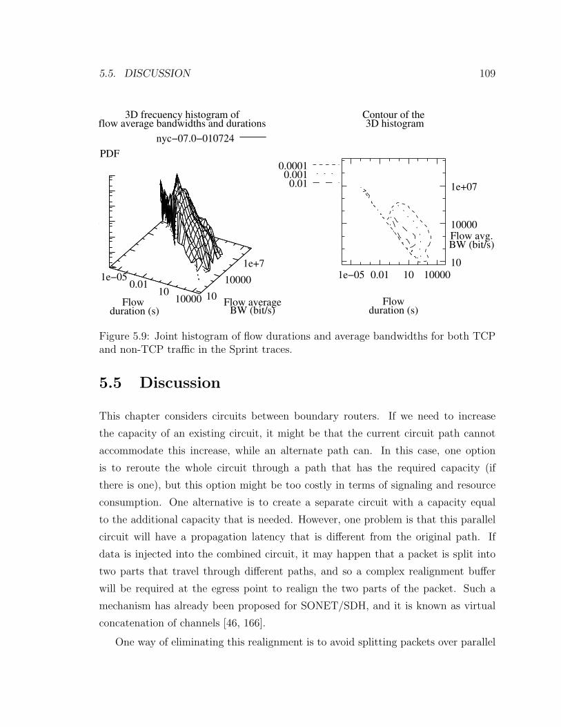
the work by Zhang et al. [189]. Figure 5.9 shows the joint histogram for the flow
duration and average bandwidth, which makes their correlation clear. Jobs with more
available bandwidth usually take less time to complete. In terms of successive arrivals,
the autocorrelation function was almost zero, and so the arrivals can be considered
5One could use the number of bytes transferred by the flow instead of the flow average bandwidth,since the latter is equal to the former divided by the flow duration.
6For TCP traffic, the correlation coefficient was between -0.137 and -0.310, whereas for non-TCPtraffic, it was between -0.089 and -0.391.

5.4. MODELING TRAFFIC TO HELP IDENTIFY THE SAFEGUARD BAND107
1e−06
1e−05
0.0001
0.001
0.01
0.1
1
0 0.01 0.02 0.03 0.04 0.05 0.06
Inve
rse
CD
F
Flow interarrival time (s)
All flows (TCP+UDP+ICMP)
nyc−07.0−010724nyc−08.0−010724pen−02.0−010905pen−05.0−010905
Figure 5.7: Inverse cumulative histogram of the flow interarrivals for both TCP andnon-TCP traffic in the Sprint traces. An exponential interarrival time would berepresented as a straight line in this graph.
independent. The flow average bandwidth and flow duration can then be modeled as
a sequence of i.i.d. 2-dimensional random variables.
Even if the correlation between the flow average bandwidth and the flow duration
is small, when the marginal distributions of the two magnitudes are used the results
of the model and the traces diverge considerably for the low overflow probabilities.
The reason is that short-duration and high-bandwidth flows occur more often in
the synthetic traces created from the marginal distributions than in the real trace,
and these flows can skew the results. Results are much closer to the trace-driven
model when using Poisson arrivals and the empirical joint distribution for the flow
duration and average rate. Figure 5.10 shows how the synthetic trace using the joint
distribution produces results that are very close to those obtained with the real trace.
This model corresponds to an MB/G/∞ system, where there are infinite par-
allel servers, arrivals are batched Poisson and service times are correlated with the

108 CHAPTER 5. COARSE CIRCUIT SWITCHING IN THE CORE
0
0.02
0.04
0.06
0.08
0.1
0.12
0.14
100 10000 1e+06 1e+08
His
togr
am fr
eque
ncy
Flow average bandwidth (bit/s)
All flows (TCP+UDP+ICMP)
nyc−07.0−010724nyc−08.0−010724pen−02.0−010905pen−05.0−010905
sj−05.0−010905sj−b−06.0−010724
0
0.02
0.04
0.06
0.08
0.1
0.12
1e−06 0.0001 0.01 1 100 10000H
isto
gram
freq
uenc
yFlow duration (s)
All flows (TCP+UDP+ICMP)
nyc−07.0−010724nyc−08.0−010724pen−02.0−010905pen−05.0−010905
sj−05.0−010905sj−b−06.0−010724
(a) (b)
Figure 5.8: Histograms of (a) the flow average bandwidth and (b) the flow durationfor both TCP and non-TCP traffic in the Sprint traces. Single-packet flows have notbeen considered.
batch size. As far as I know, there is no closed-form expression for the transition
probabilities:
p = 1 − P [N(t) − N(0) < SpT · N(0),∀t ∈ [0, T )]
= P [max{N(t) − N(0),∀t ∈ [0, T )} ≥ SpT · N(0)]
where N(t) is the number of clients in the system at time t.
In summary, we can estimate the safeguard band that is required to avoid circuit
overflows just by using the average flow rate and the joint distribution of the flow
average bandwidth and the flow duration. This information can then be used to
construct a set of curves like the one in Figure 5.10.
5.5. DISCUSSION 109
Flow avg.BW (bit/s)
3D frecuency histogram offlow average bandwidths and durations
nyc−07.0−010724
1e−050.01
1010000Flow
duration (s)10
10000
1e+7
Flow averageBW (bit/s)
1e−71e−61e−51e−40.001
0.010.1
Contour of the
0.0001 0.001 0.01
1e−05 0.01 10 10000
Flowduration (s)
10
10000
1e+07
3D histogram
Figure 5.9: Joint histogram of flow durations and average bandwidths for both TCPand non-TCP traffic in the Sprint traces.
5.5 Discussion
This chapter considers circuits between boundary routers. If we need to increase
the capacity of an existing circuit, it might be that the current circuit path cannot
accommodate this increase, while an alternate path can. In this case, one option
is to reroute the whole circuit through a path that has the required capacity (if
there is one), but this option might be too costly in terms of signaling and resource
consumption. One alternative is to create a separate circuit with a capacity equal
to the additional capacity that is needed. However, one problem is that this parallel
circuit will have a propagation latency that is different from the original path. If
data is injected into the combined circuit, it may happen that a packet is split into
two parts that travel through different paths, and so a complex realignment buffer
will be required at the egress point to realign the two parts of the packet. Such a
mechanism has already been proposed for SONET/SDH, and it is known as virtual
concatenation of channels [46, 166].
One way of eliminating this realignment is to avoid splitting packets over parallel

110 CHAPTER 5. COARSE CIRCUIT SWITCHING IN THE CORE
Sprint tracePoisson arrivals,
Empirically distributed flows1e−06
1e−05
0.0001
0.001
0.01
0.1
1
0.0001 0.001 0.01 0.1 1
Cir
cuit
over
flow
pro
babi
lity
Safeguard band relative to the peak−bandwidth envelope
Curves indexed by circuit−creation latencynyc−07.0−010724
100 ms
10 ms
1 ms
1 s
Figure 5.10: Safeguard band required for certain overflow probabilities and circuit-creation latencies for real traffic traces (solid line) and a simple traffic model (dashedline) with Poisson arrivals and flow characteristics that are drawn from an empiricaldistribution.
paths. Packets can then be recovered integrally at the tail end of each backbone circuit
and injected directly into the packet-switched part of the network. This method can
create some packet reordering within a user flow, which TCP may interpret as packet
drops due to congestion. Yet, reordering would be rare if the difference in propagation
delays between the parallel paths is smaller than the interarrival time imposed by the
access link to consecutive packets of the same flow (for 1500-byte packets, it is 214 ms
for 56-Kbit/s access links, and 8 ms for 1.5-Mbit/s access links). One possible solution
is to equalize the delay using a fixed-size buffer at the end of one of the sub-circuits.
However, this buffer may not be necessary because, as reported recently [17], TCP is
not significantly affected by occasional packet reordering in a network.
It should be pointed out that the definition used here for circuit overflow is rather
strict, and it represents an upper bound on the packet drop rate. In general, the

5.6. CONCLUSIONS AND SUMMARY OF CONTRIBUTIONS 111
ingress boundary router will have buffers at the head end of each backbone circuit,
which will absorb short fluctuations in the flow rate between boundary routers. For
this reason, in the measurements in Figures 5.5 and 5.10, all single-packet flows
were ignored. The buffer at the head end will also allow the system to achieve
some statistical multiplexing between active flows; something that TCP Switching in
Chapter 4 could not achieve. However, as mentioned in Chapter 3, this statistical
multiplexing will not necessarily lead to a smaller response time because the flow
peak rate will still be capped by the access link.
The approach presented in this chapter does not specify any signaling mechanism
and does not impose any requirements on it. One could use existing mechanisms
such as the ones envisioned by GMPLS [7] or OIF [13], which will be described in
Chapter 6. This method can also be used in conjunction with TCP Switching to
control an optical backbone with an electronic outer core and an optical inner core.
TCP Switching would control the outer fine-grain electronic circuit switches and
would provide the information that is used to control the inner coarse-grain optical
circuit switches.
5.6 Conclusions and summary of contributions
This Chapter has discussed how to monitor user flows to predict when more band-
width is needed between boundary routers of a circuit-switched cloud in the Internet.
It has also developed a simple model that can be used to estimate safeguard bands
that compensate for slow circuit-creation mechanisms.
The most important recommendation of this chapter is that the signaling used
to establish a circuit should be as fast as possible. Otherwise, the safeguard band
becomes very large. An alternative reading of this recommendation is that the es-
tablishment of a circuit should be done simultaneously on all nodes along the path,
without having to wait for any confirmation from the upstream or downstream nodes.
Moreover, slow crossconnect technologies (such as MEMS mirrors) should only be
used if they can provide a very large switching capacity at a low cost, such that it
can accommodate the additional safeguard band.