106

CHAPTER 5

ANALYSIS OF FLOW IN NOZZLE SYSTEM USING

COMPUTATIONAL FLUID DYNAMICS

5.0 INTRODUCTION

The air velocity from nozzle system is validated computationally using

CFD. Experimentally the outlet velocity of air from the nozzle system is

determined and discussed in chapter 4. Applications of CFD, governing

equations, meshing methods, importance of software GAMBIT 2.3.16

and FLUENT 6.3.26 in the present research, are discussed in this

chapter. Boundary conditions like compressibility, turbulence, pressure,

temperature at the inlet of the nozzle system, etc, are discussed. Flow

through outer convergent nozzle and multiple nozzle system without

heaters and with heaters are analyzed. In the analysis, the velocity

variation, pressure variation, turbulent kinetic energy variation, etc, are

also discussed. Effect of ambient temperature suited to the climatic

conditions of India is also presented in this chapter.

5.1 APPLICATIONS AND BENEFITS OF CFD

The major applications of CFD are stated below. (Anderson, 1995)

• Aerodynamic design of impeller blades of axial flow compressors,

centrifugal compressors.

107

• Fluid flow pattern in heat transfer equipment like heat exchangers,

stirred reactors, ducts, pulverizing machines, boilers, steam

turbine, gas turbine and hydraulic turbines.

• Fluid flow and heat transfer in the electronic equipment like micro

channels and control panels.

• Meteorologists and oceanographers to foretell wind and water

currents. Hydrologists to forecast the effects of changes to ground

water.

• Petroleum engineers to design optimum oil-recovery strategies.

• In analyzing the heat transfer rates in various components of

automobile vehicles. The analysis will be helpful in analyzing the

performance of the vehicle.

• In the study of blood circulation of the human body, tooth

analysis using finite element method.

Benefits: (Walsi89, 1998)

• Low Cost

• High speed in problem solving

• Complete information of the analysis

• Ability to simulate realistic conditions

• Ability to simulate ideal conditions

• Reduction of failure risks

108

5.2 STRATEGY OF CFD

The strategy of CFD is to replace the continuous domain with a

discrete domain using a grid. In the discrete domain, variable is defined

at grid points. In CFD, the flow can be analyzed for the relevant flow

variables only at grid points. The values at other locations are

determined by interpolating the values occurred at the grid points.

Governing equations define the variables in the discrete form. The

discrete system is the largest set of coupling algebraic equations in the

form of discrete variables. Setting up the discrete system and solving it

involves an extraordinarily large number of iterations to converge the

solution. (Wesseling90, 2000)

5.3 GOVERNING EQUATIONS OF CFD

In CFD, the physical aspect of any fluid flow is governed by three

principles. (Anderson, 1995)

• Conservation of mass

• Conservation of momentum

• Conservation of energy

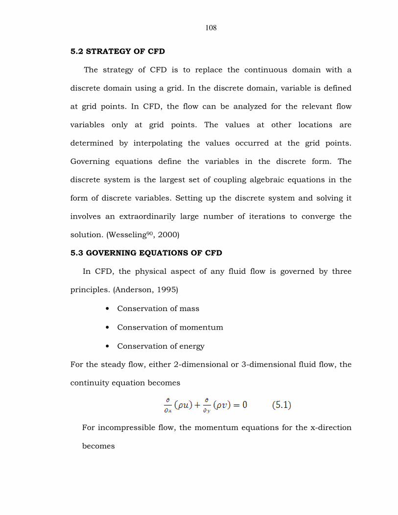
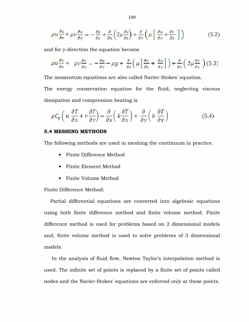
For the steady flow, either 2-dimensional or 3-dimensional fluid flow, the

continuity equation becomes

For incompressible flow, the momentum equations for the x-direction

becomes

109

+

and for y-direction the equation become

The momentum equations are also called Navier-Stokes' equation.

The energy conservation equation for the fluid, neglecting viscous

dissipation and compression heating is

5.4 MESHING METHODS

The following methods are used in meshing the continuum in practice.

• Finite Difference Method

• Finite Element Method

• Finite Volume Method

Finite Difference Method:

Partial differential equations are converted into algebraic equations

using both finite difference method and finite volume method. Finite

difference method is used for problems based on 2 dimensional models

and, finite volume method is used to solve problems of 3 dimensional

models.

In the analysis of fluid flow, Newton Taylor’s interpolation method is

used. The infinite set of points is replaced by a finite set of points called

nodes and the Navier-Stokes' equations are enforced only at these points.

110

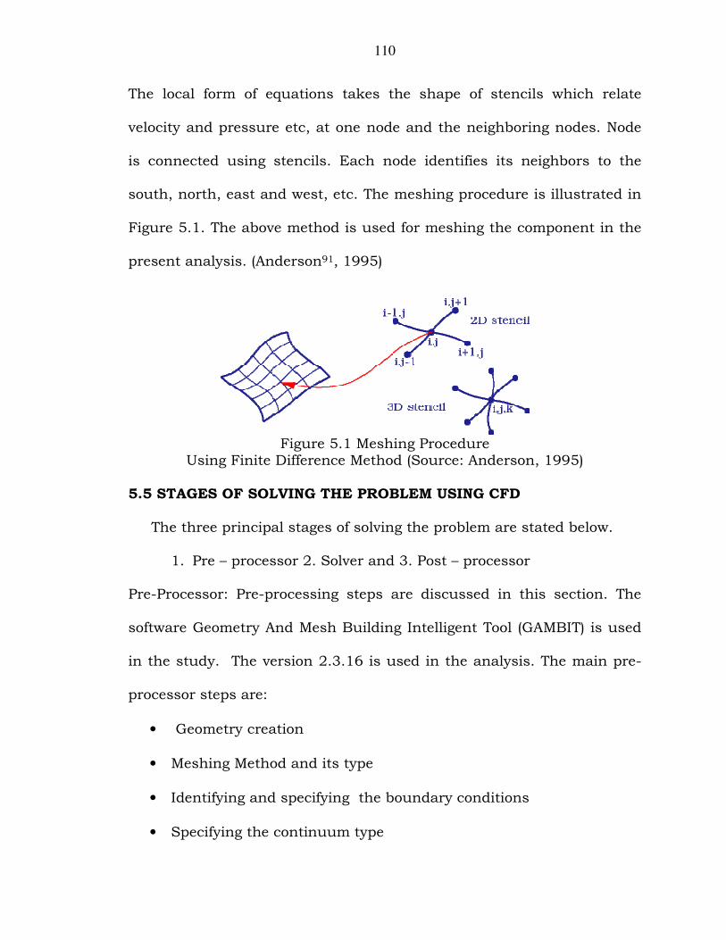
The local form of equations takes the shape of stencils which relate

velocity and pressure etc, at one node and the neighboring nodes. Node

is connected using stencils. Each node identifies its neighbors to the

south, north, east and west, etc. The meshing procedure is illustrated in

Figure 5.1. The above method is used for meshing the component in the

present analysis. (Anderson91, 1995)

Figure 5.1 Meshing Procedure Using Finite Difference Method (Source: Anderson, 1995)

5.5 STAGES OF SOLVING THE PROBLEM USING CFD

The three principal stages of solving the problem are stated below.

1. Pre – processor 2. Solver and 3. Post – processor

Pre-Processor: Pre-processing steps are discussed in this section. The

software Geometry And Mesh Building Intelligent Tool (GAMBIT) is used

in the study. The version 2.3.16 is used in the analysis. The main pre-

processor steps are:

• Geometry creation

• Meshing Method and its type

• Identifying and specifying the boundary conditions

• Specifying the continuum type

111

The mesh for 2-dimensional analysis includes quadrilateral and

triangular mesh. Quadrilateral type meshing indicates the square or

rectangle cell. But, the triangular meshing indicates the triangular cell.

Out of them, quadrilateral meshing is preferred due to more accuracy.

Triangular meshing yields better results when the skew angle of the

triangle is 600. Continuum type may be either solid or fluid.

The time taken for solving the problem may be increased due to

increase in number of cells. But, it is compensated by increasing the

accuracy levels. The main disadvantage in solving the fluid flow problems

through CFD is the ram capacity of the computer system. It also depends

upon the shape of the object. It may require the capacity of 4 GB. For

complex components, the ram capacity may exceed 8 GB also.

(Wesseling90, 2000).

Solver:

At the outset, the numerical methods form the basis of the solver to

converge the solution. Solver performs the following events.

• Approximation of the unknown flow variables by means of

elementary functions

• Meshing by substation of the approximations into the governing

flow equations and subsequent mathematical manipulations

• Solution of the algebraic equations

112

Post-Processor:

Packages of computational dynamics are now equipped with versatile

data visualisation tools: they include,

• Domain geometry and grid display

• Vector plots

• Line and shaded contour plots

• 2D and 3D surface plots

• Particle tracking

• Animation view

• Colour postscript output

5.6 COMPRESSIBLE FLOW AND INCOMPRESSIBLE FLOW

The flow of fluid with invariant density is called incompressible fluid

flow. An ideal gas behaves like incompressible flow. If, the density of

flowing fluid is varied then such fluid flow is called compressible fluid

flow. Flow can also be classified based on Mach number. If Mach number

is more than 0.3, then the flow can be treated as compressible fluid flow.

If it lies in the range of 0 to 0.3, then the flow can be treated as

incompressible fluid flow. Incompressible fluid flow is governed mainly by

the conservation of mass and conservation of momentum equations. But

compressible fluid flow is governed by conservation of energy equation.

The flow of gas through open pipe system either internally or externally

can be treated as compressible fluid flow if Mach number exceeds 0.3.

Compressible flow includes flow of air around bodies such as the wings

113

of an airplane. Results may vary by 5%, if compressible flow is

considered. (Anderson91, 1990)

5.7 BOUNDARY CONDITIONS IN THE ANALYSIS

The following boundary conditions are considered in analyzing the

fluid flow through nozzle system. They are:

(i) Incompressible fluid flow (ii) Turbulent fluid flow

(ii) Atmospheric pressure at the inlet of nozzle system

(iii)Axis symmetry

(iv) Neglecting wall viscous forces

Incompressible fluid flow:

Experimentally, the velocity of air at the outlet of the nozzle system is

measured using rotating disc type anemometer. It is 8.5 m/s at a

minimum and 20.3 m/s at maximum in all modules. The compressibility

is defined based on Mach number. It is the ratio of velocity of an object to

velocity of sound in the surrounding medium. Velocity of sound at sea

level is 340.3 m/s. Thus, minimum and maximum Mach number

becomes 0.0249 and 0.0596 respectively. It is less than 0.3. If Mach

number is more than 0.3, the flow can be treated as compressible fluid

flow. Hence, the flow chosen is incompressible in the analysis.

Turbulent fluid flow:

The flow in the analysis becomes turbulent. Reynolds number is

determined to know whether the flow is turbulent or laminar. As stated

in the section A.4, air with minimum velocity 8.5 m/s, from the nozzle of

114

inlet diameter 0.6 meter and at 270C has Reynolds number 490100. But,

air with maximum velocity 20.3 m/s, from nozzle inlet diameter of 0.15

meter at temperature 36.90C has Reynolds number 182142.

In the above two cases, Reynolds number lies above 4000. For a fully

developed flow through a circular pipe, the flow becomes turbulent since,

Reynolds number exceeds 4000. Hence, in the analysis the flow is

treated turbulent. (Modi and Seth92, 2010)

Inlet velocity, inlet Pressure and inlet temperature:

Nozzle system is assembled with wind tunnel. Air passes through wind

tunnel and then through nozzle system. Wind tunnel produces air at

velocity of 8.5 m/s. Hence, this velocity becomes inlet velocity for nozzle

system. The pressure chosen is atmospheric pressure i.e., 0.9669 Pa. The

temperature of air is approximately at 270C in the case of single nozzle

system and multiple nozzle system. But, air is at 36.9 0C in multiple nozzle

system with heaters.

Axis symmetry:

The nozzle is a continuous varying cross section from inlet to outlet.

Its geometry is symmetrical to the axis. Hence, the flow is analyzed using

2 – dimensional geometry model.

Wall viscous force:

Wall resists fluid flow. It is approximately stationary at inner walls of

nozzle.

115

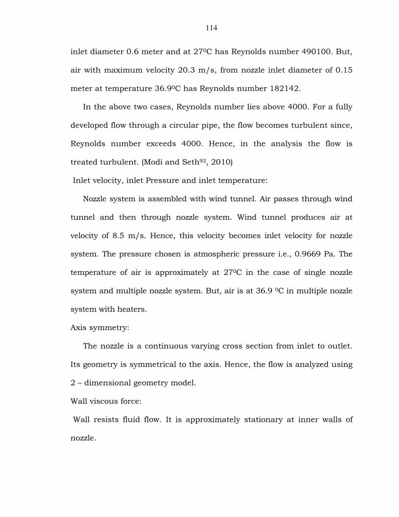
5.8 FLOW ANALYSIS IN OUTER CONVERGENT NOZZLE

Geometry of the nozzle is modeled using GAMBIT 2.3.16 as per the

following dimensions.

Inlet diameter : 0.6 meter

Outlet diameter : 0.45 meter

Length of the nozzle : 0.45 meter

The analysis is carried out under various mesh sizes namely 100 x

150, 150 x 200, 400 x 500, etc. The analysis indicates that, on the last

two occasions, the air velocity at the outlet of the nozzle is come close.

Hence, the solution is said to be made grid independent. The mesh size

of 400 x 500 is considered for further analysis. The outer/single nozzle

after meshing is illustrated in Figure 5.2. After meshing, total number of

cells becomes 200000 with the total number of faces 400900. The total

number of nodes becomes 200901.

Figure 5.2 Meshing of Outer Nozzle

116

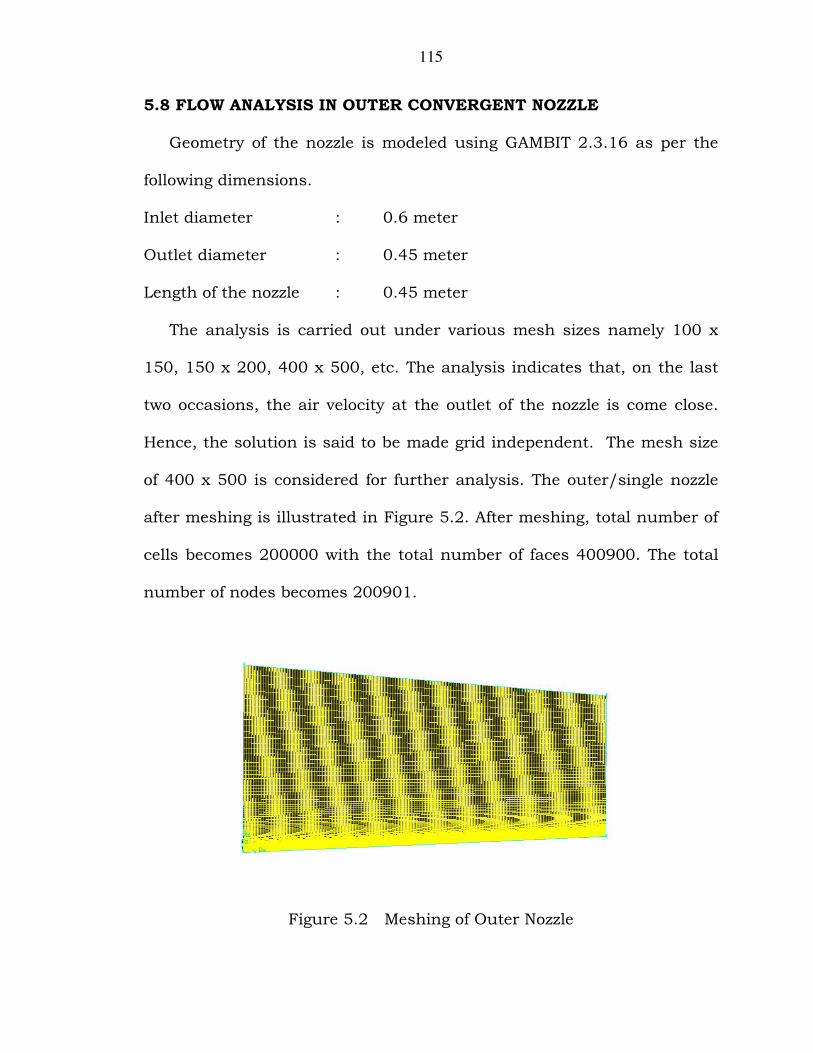
The meshing is fine near the axis and coarse at walls. Solver package

has taken 204 iterations to converge the solution. Figure 5.3 illustrates

the solution convergence of the analysis.

Figure 5.3 Solution Convergence of Outer Nozzle

Second order equations of velocities in x- direction, velocity in y-

direction, continuity, k (turbulent kinetic energy), Epsilon (Turbulent

dissipation rate) are considered in converging the solution. The residual

of convergence can be read from Y-axis. X-axis indicates the total

number of iterations to converge the solution. Solution is converged with

accuracy more than 99.99%.

Boundary Conditions

In this analysis boundary conditions are incompressible, turbulent, axis

symmetry with wall viscous flow having inlet air velocity 8.5 m/s and at

pressure and temperature respectively at 0.9669 Pa and 27 0C.

117

5.8.1 Study of Various Parameters in Outer Nozzle Velocity

Variations

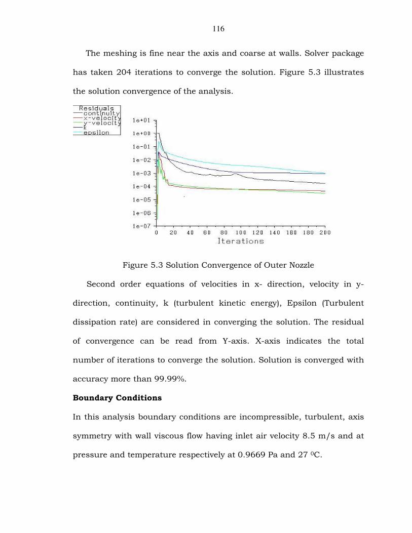
Solver has plotted variations of velocity through the nozzle system. Air

enters the nozzle at a velocity of 8.5 m/s. But it leaves at velocity of 15.2

m/s. Velocity variation zones are illustrated in Figure 5.4. Velocity of air

increases, from inlet to outlet. The zone in red color indicates the velocity

of air at the outlet. The zone in blue color indicates velocity of air at the

inlet of nozzle system.

Figure 5.4 Velocity variations in various Zones of Outer Nozzle

But, experimentally velocity of air at the outlet of nozzle system is 15.0

m/s. The percentage of deviation from computational velocity is 1.33%.

Velocity variations at various positions:

The total length of outer convergent nozzle is 0.6 m. Velocity is varied

from 8.5 m/s at inlet to 15.2 m/s at the outlet. The velocity of air at

118

various locations in the nozzle system is illustrated in Figure 5.5.

Approximately at a distance of 0.1 m from inlet, the fluctuations in

velocity occurred. The reason may be due to swirl among various air

particles.

Figure 5.5 Air Velocities at Various Positions in Outer Nozzle

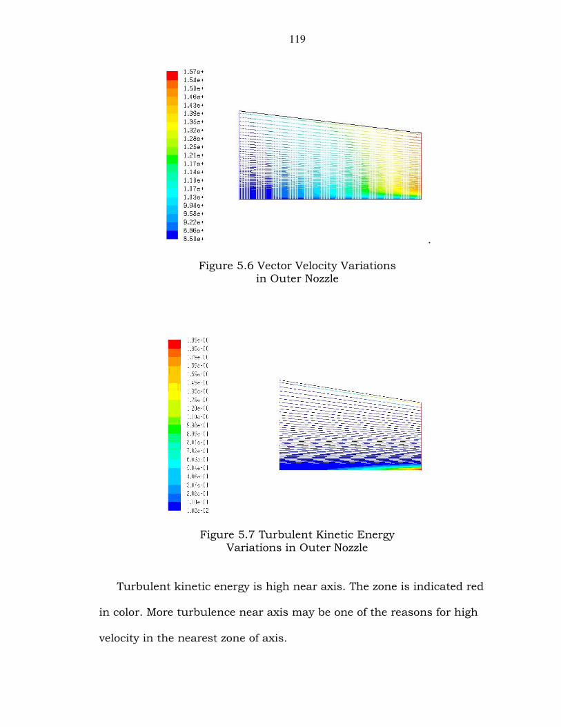
Velocity vector variations and turbulent kinetic energy variations

Velocity vector indicates both magnitude and direction of the velocity.

Its variations are illustrated in Figure 5.6. The magnitude of air velocity

is more at the outlet and that too, near axis. The zone is indicated red in

color. Turbulent kinetic energy variations are illustrated in Figure 5.7. It

is measured in terms of m2/sec2. The nozzle system exerts high

turbulent kinetic energy near the axis.

119

.

Figure 5.6 Vector Velocity Variations in Outer Nozzle

Figure 5.7 Turbulent Kinetic Energy Variations in Outer Nozzle

Turbulent kinetic energy is high near axis. The zone is indicated red

in color. More turbulence near axis may be one of the reasons for high

velocity in the nearest zone of axis.

120

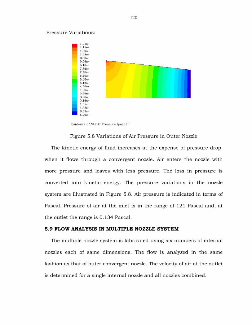
Pressure Variations:

Figure 5.8 Variations of Air Pressure in Outer Nozzle

The kinetic energy of fluid increases at the expense of pressure drop,

when it flows through a convergent nozzle. Air enters the nozzle with

more pressure and leaves with less pressure. The loss in pressure is

converted into kinetic energy. The pressure variations in the nozzle

system are illustrated in Figure 5.8. Air pressure is indicated in terms of

Pascal. Pressure of air at the inlet is in the range of 121 Pascal and, at

the outlet the range is 0.134 Pascal.

5.9 FLOW ANALYSIS IN MULTIPLE NOZZLE SYSTEM

The multiple nozzle system is fabricated using six numbers of internal

nozzles each of same dimensions. The flow is analyzed in the same

fashion as that of outer convergent nozzle. The velocity of air at the outlet

is determined for a single internal nozzle and all nozzles combined.

121

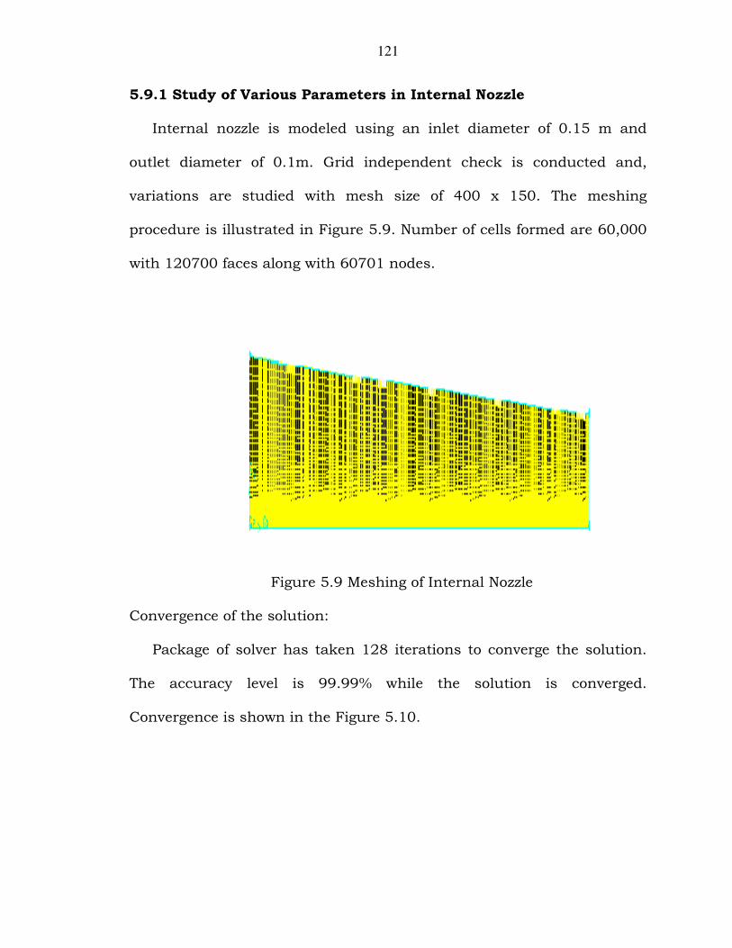
5.9.1 Study of Various Parameters in Internal Nozzle

Internal nozzle is modeled using an inlet diameter of 0.15 m and

outlet diameter of 0.1m. Grid independent check is conducted and,

variations are studied with mesh size of 400 x 150. The meshing

procedure is illustrated in Figure 5.9. Number of cells formed are 60,000

with 120700 faces along with 60701 nodes.

Figure 5.9 Meshing of Internal Nozzle Convergence of the solution:

Package of solver has taken 128 iterations to converge the solution.

The accuracy level is 99.99% while the solution is converged.

Convergence is shown in the Figure 5.10.

122

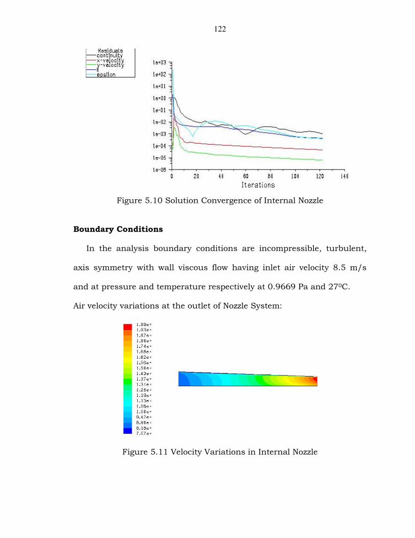
Figure 5.10 Solution Convergence of Internal Nozzle

Boundary Conditions

In the analysis boundary conditions are incompressible, turbulent,

axis symmetry with wall viscous flow having inlet air velocity 8.5 m/s

and at pressure and temperature respectively at 0.9669 Pa and 270C.

Air velocity variations at the outlet of Nozzle System:

Figure 5.11 Velocity Variations in Internal Nozzle

123

The variations of velocity are illustrated in Figure 5.11 for the internal

nozzle. Air enters into the nozzle at 8.5 m/s and leaves with 19.89 m/s.

The zone of high velocity is represented red in color. Experimental outlet

velocity of air is 19.2 m/s. Hence, the experimental velocity deviated from

computational velocity by 3.59%.

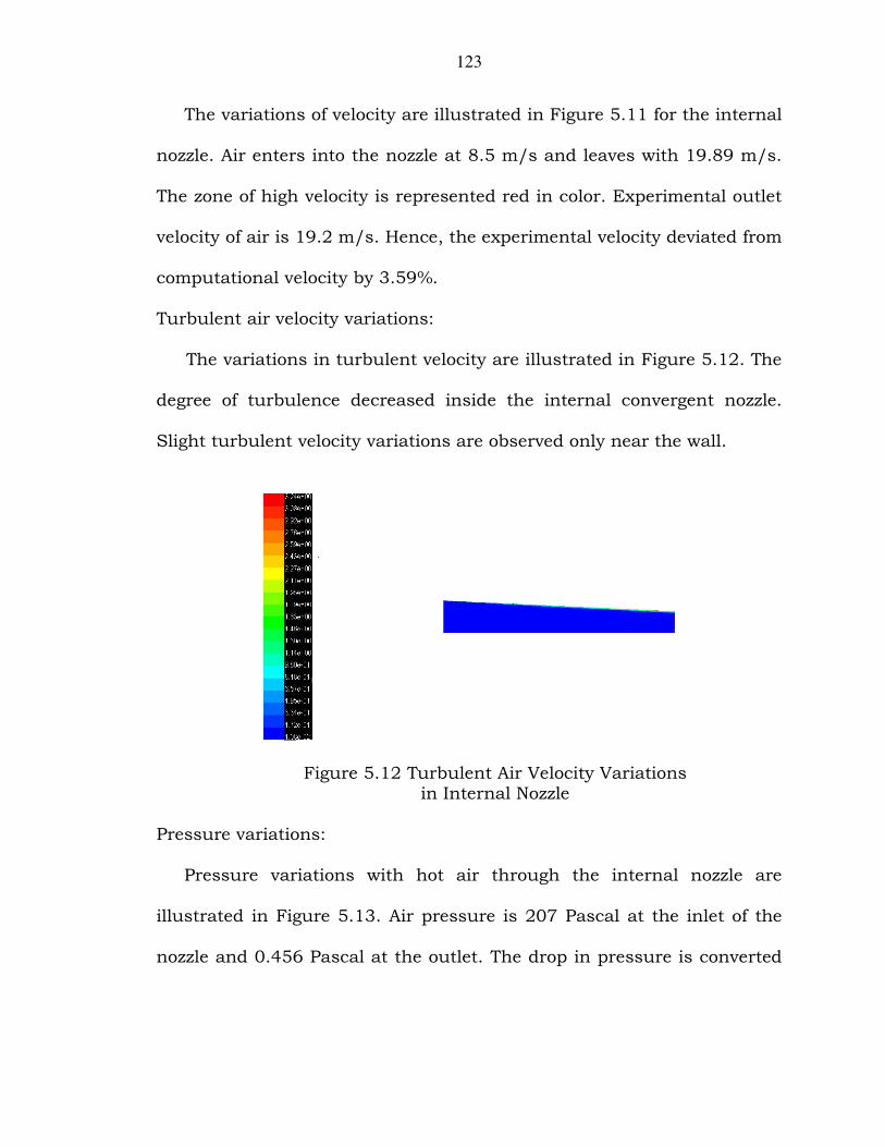
Turbulent air velocity variations:

The variations in turbulent velocity are illustrated in Figure 5.12. The

degree of turbulence decreased inside the internal convergent nozzle.

Slight turbulent velocity variations are observed only near the wall.

Figure 5.12 Turbulent Air Velocity Variations in Internal Nozzle

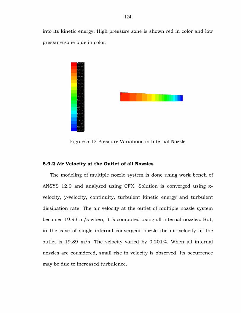
Pressure variations:

Pressure variations with hot air through the internal nozzle are

illustrated in Figure 5.13. Air pressure is 207 Pascal at the inlet of the

nozzle and 0.456 Pascal at the outlet. The drop in pressure is converted

124

into its kinetic energy. High pressure zone is shown red in color and low

pressure zone blue in color.

Figure 5.13 Pressure Variations in Internal Nozzle

5.9.2 Air Velocity at the Outlet of all Nozzles

The modeling of multiple nozzle system is done using work bench of

ANSYS 12.0 and analyzed using CFX. Solution is converged using x-

velocity, y-velocity, continuity, turbulent kinetic energy and turbulent

dissipation rate. The air velocity at the outlet of multiple nozzle system

becomes 19.93 m/s when, it is computed using all internal nozzles. But,

in the case of single internal convergent nozzle the air velocity at the

outlet is 19.89 m/s. The velocity varied by 0.201%. When all internal

nozzles are considered, small rise in velocity is observed. Its occurrence

may be due to increased turbulence.

125

5.10 FLOW ANALYSIS USING ELECTRIC HEATERS

In the earlier section, the flow through multiple nozzle system is

analyzed without electric heaters. In the same fashion, the analysis is

carried out when electric heaters are working. The temperature of air is

increased to 36.90C from 270C. Hence, in the present study the

temperature of air at the inlet of the nozzle system becomes 36.90C. In

the analysis, a single internal nozzle system is considered.

Boundary Conditions

In the analysis boundary conditions are are incompressible, turbulent,

axis symmetry with wall viscous flow having inlet air velocity 8.5 m/s

and at pressure and temperature respectively at 0.9669 Pa and 370C.

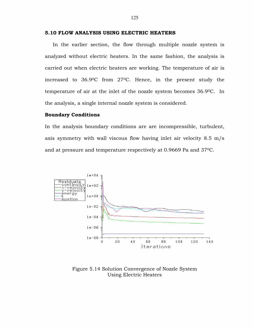
Figure 5.14 Solution Convergence of Nozzle System Using Electric Heaters

126

Grid independent test is conducted and lattice is divided using mesh size

400 x 150. The convergence process has taken 134 iterations and is

illustrated in Figure 5.14. The solution converged with an accuracy level

of 99.99%.

5.10.1 Study of Various Parameters Using Electric Heaters

When heaters are used velocity, turbulent kinetic energy and

pressure variations are studied in this section.

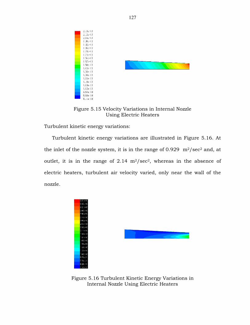
Velocity variations:

At outlet, air velocity increased to 20.60 m/s when air at a

temperature of 36.90C is passed through the nozzle system. The velocity

variations are illustrated in Figure 5.15. Maximum velocity region is

represented in the red color.

Velocity of air at the inlet of the nozzle system is 8.5 m/s and, it

increases to 20.60 m/s at outlet. But, in the absence of electric heaters,

the air velocity is 19.89 m/s. It increases by 3.5 %. It is appealing to

know that in increasing the kinetic energy of air, no moving parts are

used. Hence, it can be stated that multiple nozzle system can convert a

portion of wind’s heat energy into kinetic energy. If the multiple nozzle

system is optimized, the air velocities at outlet can further be increased.

Experimental air velocity at the outlet of multiple nozzle system is 20.30

m/s. computationally it is 20.6 m/s. Experimental velocity varied by

1.87 percentage.

127

Figure 5.15 Velocity Variations in Internal Nozzle Using Electric Heaters

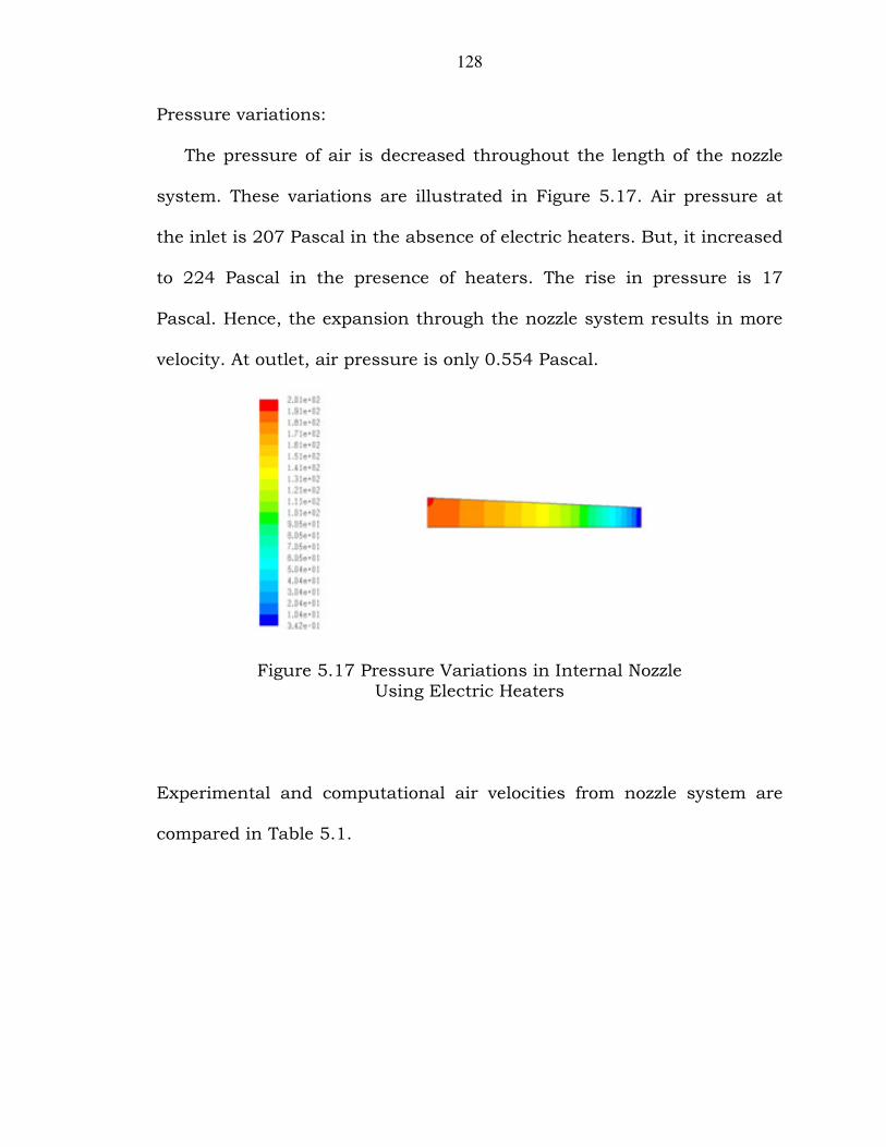
Turbulent kinetic energy variations:

Turbulent kinetic energy variations are illustrated in Figure 5.16. At

the inlet of the nozzle system, it is in the range of 0.929 m2/sec2 and, at

outlet, it is in the range of 2.14 m2/sec2, whereas in the absence of

electric heaters, turbulent air velocity varied, only near the wall of the

nozzle.

Figure 5.16 Turbulent Kinetic Energy Variations in Internal Nozzle Using Electric Heaters

128

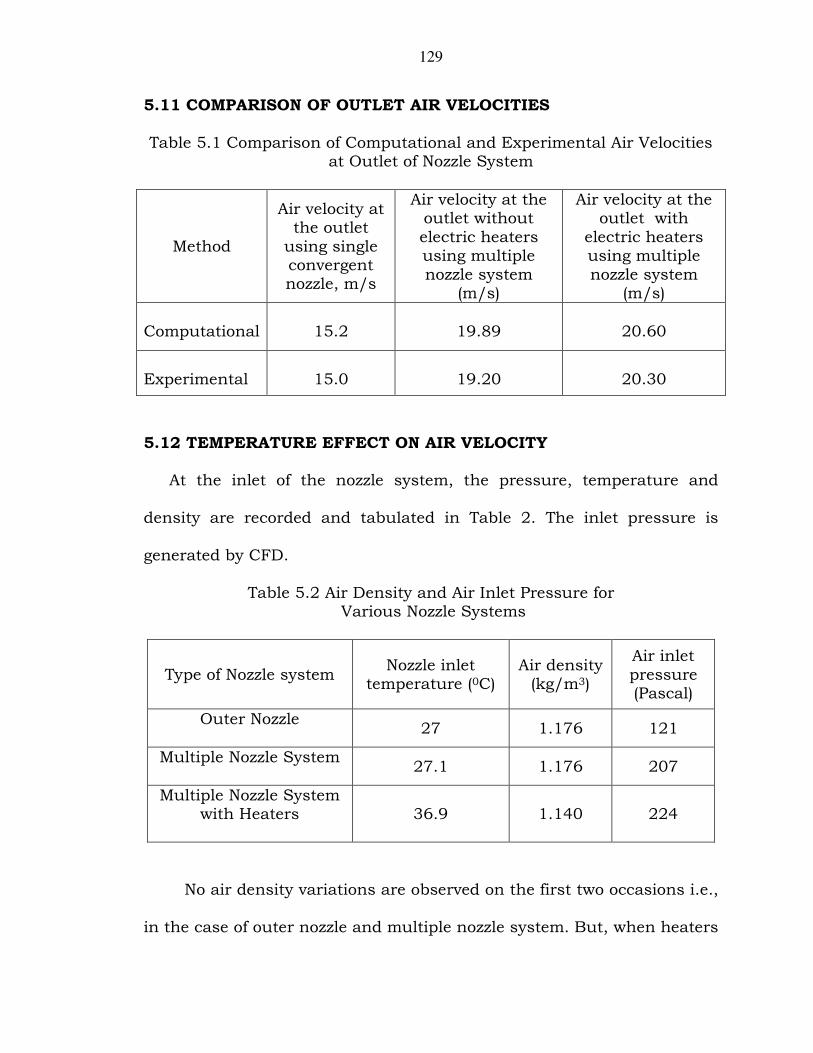
Pressure variations:

The pressure of air is decreased throughout the length of the nozzle

system. These variations are illustrated in Figure 5.17. Air pressure at

the inlet is 207 Pascal in the absence of electric heaters. But, it increased

to 224 Pascal in the presence of heaters. The rise in pressure is 17

Pascal. Hence, the expansion through the nozzle system results in more

velocity. At outlet, air pressure is only 0.554 Pascal.

Figure 5.17 Pressure Variations in Internal Nozzle Using Electric Heaters

Experimental and computational air velocities from nozzle system are

compared in Table 5.1.

129

5.11 COMPARISON OF OUTLET AIR VELOCITIES

Table 5.1 Comparison of Computational and Experimental Air Velocities at Outlet of Nozzle System

Method

Air velocity at the outlet

using single convergent nozzle, m/s

Air velocity at the outlet without electric heaters using multiple nozzle system

(m/s)

Air velocity at the outlet with

electric heaters using multiple nozzle system

(m/s)

Computational

15.2

19.89

20.60

Experimental

15.0

19.20

20.30

5.12 TEMPERATURE EFFECT ON AIR VELOCITY

At the inlet of the nozzle system, the pressure, temperature and

density are recorded and tabulated in Table 2. The inlet pressure is

generated by CFD.

Table 5.2 Air Density and Air Inlet Pressure for Various Nozzle Systems

Type of Nozzle system Nozzle inlet

temperature (0C) Air density

(kg/m3)

Air inlet pressure (Pascal)

Outer Nozzle

27 1.176 121

Multiple Nozzle System

27.1 1.176 207

Multiple Nozzle System with Heaters

36.9 1.140 224

No air density variations are observed on the first two occasions i.e.,

in the case of outer nozzle and multiple nozzle system. But, when heaters

130

are applied, significant change in temperature occurred. The decrease in

air density is found when hot air is passed. It is reduced by 3.06%.

Due to more contraction at inlet of the multiple nozzle system the air

pressure increases. When heaters are applied, the inlet air pressure is

increased to 224 Pascal from 207 Pa. The rise in air inlet pressure is

8.21%. If the inlet air pressure increases, the air velocity from nozzle

system increases due to more expansion. Hence, the air velocity at the

outlet of the multiple nozzle system is increased. Practically, it is

increased by 5.72%.

In the equation 3.12, the power in wind is directly proportional to the

air density and Vi3. The effect of air velocity dominates the fall in density.

Hence, more power in wind is found, when heaters are applied.

5.13 STUDIES WITH HOT AIR AT 470C

Ambient air ranges from 450C to 500C in summer. The effect of this

temperature is studied in this section. The temperature at the inlet of

multiple nozzle system chosen is 470C. The effect of temperature in

increasing the air velocity at outlet is studied in this section. It is studied

only computationally.

Solution convergence:

Solution convergence is illustrated in Figure 5.18. Eighty iterations are

taken in converging the solution.

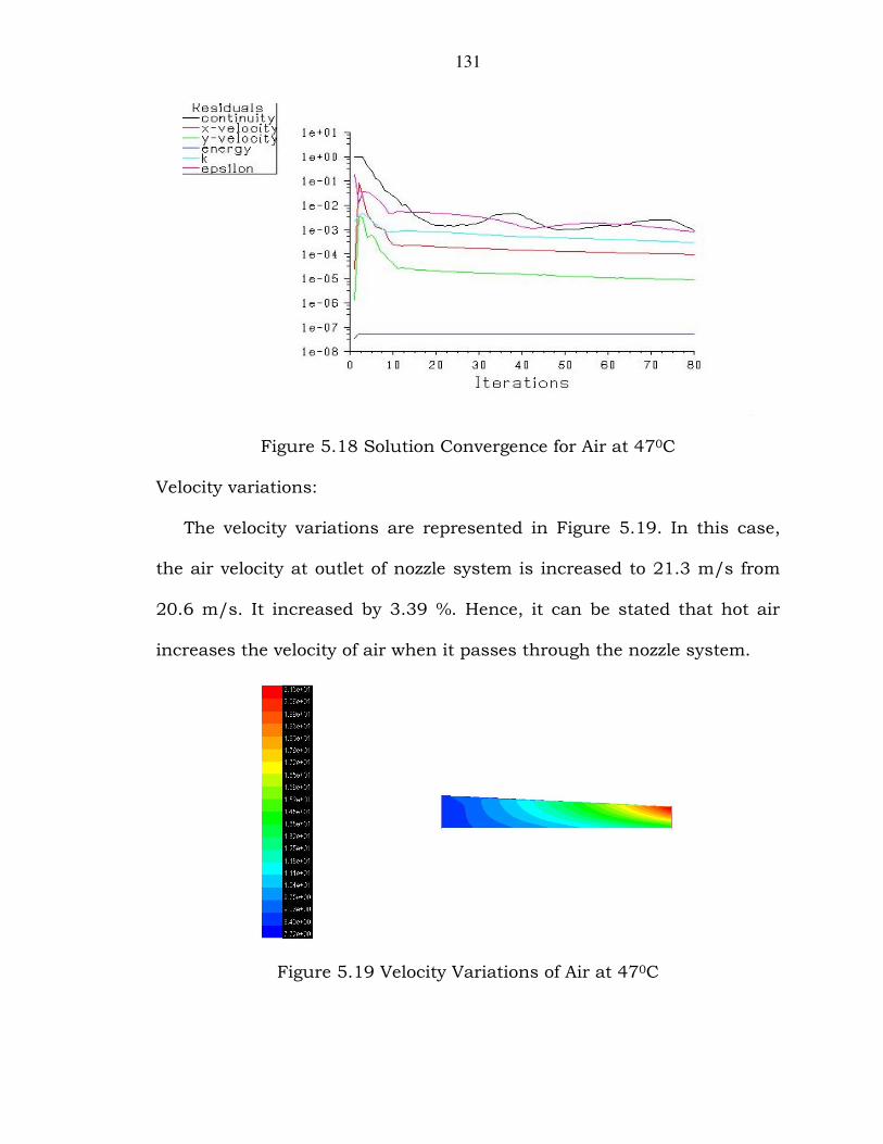
131

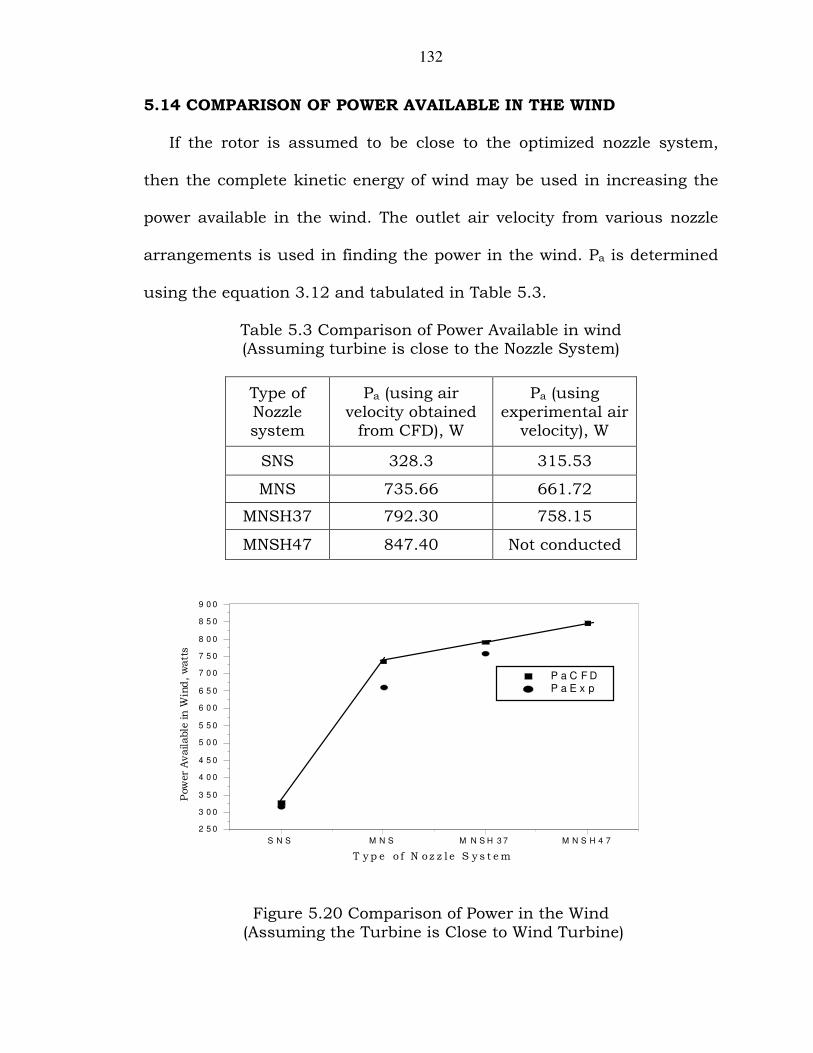
Figure 5.18 Solution Convergence for Air at 470C Velocity variations:

The velocity variations are represented in Figure 5.19. In this case,

the air velocity at outlet of nozzle system is increased to 21.3 m/s from

20.6 m/s. It increased by 3.39 %. Hence, it can be stated that hot air

increases the velocity of air when it passes through the nozzle system.

Figure 5.19 Velocity Variations of Air at 470C

132

5.14 COMPARISON OF POWER AVAILABLE IN THE WIND

If the rotor is assumed to be close to the optimized nozzle system,

then the complete kinetic energy of wind may be used in increasing the

power available in the wind. The outlet air velocity from various nozzle

arrangements is used in finding the power in the wind. Pa is determined

using the equation 3.12 and tabulated in Table 5.3.

Table 5.3 Comparison of Power Available in wind (Assuming turbine is close to the Nozzle System)

Type of Nozzle system

Pa (using air velocity obtained

from CFD), W

Pa (using experimental air

velocity), W

SNS 328.3 315.53

MNS 735.66 661.72

MNSH37 792.30 758.15

MNSH47 847.40 Not conducted

S N S M N S M N S H 3 7 M N S H 4 7

2 5 0

3 0 0

3 5 0

4 0 0

4 5 0

5 0 0

5 5 0

6 0 0

6 5 0

7 0 0

7 5 0

8 0 0

8 5 0

9 0 0

Pow

er A

vaila

ble

in W

ind

, w

atts

T y p e o f N oz z l e S y s t e m

P a C F D P a E x p

Figure 5.20 Comparison of Power in the Wind (Assuming the Turbine is Close to Wind Turbine)

133

Power available through wind in CFD is compared with experimental

values. The variations are shown in Figure 5.20.

5.15 SUMMARY AND CONCLUSIONS

Computationally the air velocity increased from 8.5 m/s to 15.2 m/s

when outer convergent nozzle is used. Multiple nozzle system increases

velocity of air to 19.89 m/s in the absence of electric heaters. But, when

temperature of air is increased approximately by 10 0C the air velocity is

further increased to 20.6 m/s. If the temperature of air is increased to

470C, the air velocity further increases to 21.3 m/s. Experimental

velocities of air for outer convergent nozzle, multiple nozzle system

without heaters and with heaters are compared. Pressure variations and

turbulent kinetic energy variations are also studied for the flow through

nozzle system.