1

Chapter 5: An Econometric Analysis of Agricultural Production, Focusing on the

Shadow Price of Groundwater: Policies Towards Socio-Economic Sustainability.

1Koundouri, P.,

1Dávila, O.G.,

1Anastasiou, Y.,

1Antypas, A.,

1Mavrogiorgis, T.,

12Mousoulides, A.,

1Mousoulidou, M.,

1Vasiliou, K.

1Athens University of Economics and Business, GREECE

2Intercollege Larnaca, CYPRUS

Abstract The focus of Chapter 5 is on the agricultural sector in the Asopos catchment as it

has a significant impact on the status of water in the area. In particular, the aim of the chapter

is to estimate the farmers’ valuation of groundwater’s shadow price for the region of Asopos.

In order to achieve that, an agricultural micro-economic data-set from the catchment has been

collected through the use of a detailed agricultural questionnaire. As it will be explained in

the chapter, the questionnaire focuses on collecting information regarding cultivations,

production structures and use of groundwater for irrigation. The objective of the micro-

econometric analysis is to uncover patterns of groundwater use and farm efficiency. The

chapter presents the derived estimates that make possible the analysis of the impact of

different economic policies, -which will be used for the implementation of an optimal,

sustainable and integrated water policy- on farmers' profits and social welfare. The chapter

finishes with policy recommendations based on the principle of socio-economic sustainability

that assures both economic efficiency of farms and concludes with the estimation of

groundwater for irrigation shadow price and how this can be used in the design of pumping

taxes to reduce pollution and to increase farms efficiency.

Keywords Shadow price of groundwater, Groundwater use, Farm efficiency, Irrigation,

Agricultural production

2

1. Introduction

The project aims to evaluate impacts of implementing the EU water directive requiring full

cost recovery by 2015. The use of groundwater by farmers located above an aquifer is a very

common situation in irrigated agriculture. In such case an estimate of groundwater’s shadow

price can be used to value the stock of water in green accounting calculations, to help design

pumping taxes in order to mitigate externalities associated with groundwater use (Howe,

2002). The Asopos watershed has multiple uses and has significant industrial water pollution

and aquifer depletion. Farmers are using pumps illegally. There are concerns for

contamination of agricultural products from polluted water (potatoes for example). Based on

the data provided in Appendix A, it appears that wheat, potato and olive production are

distinct, monoculture systems (with potato irrigated). These crops represent about 80% of

total cultivated area. The other major land use is a mix of crops that are mostly irrigated

vegetables (about 20% of the cultivated area). Thus, the overall population could be modelled

as four strata: 1) rainfed wheat farms; rainfed olive farms; irrigated potato farms; irrigated

vegetable/mixed crop farms. More information on the local farms features is presented in

Appendix A. The following sections will deal with the estimation of groundwater’s shadow

price. In section 1, the distance function in production theory is analysed. Section 2 presents

the econometric specification, empirical estimation, and results of the estimation of

groundwater’s shadow price.

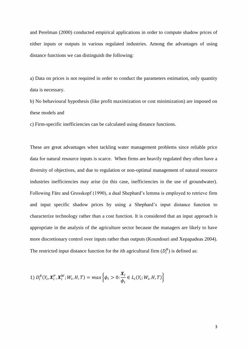
2. The Distance Functions in Production Theory

The seminal work by Shephard (1970) provided the theoretical foundations on distance

functions in production theory. Grosskopf and Hayes (1993), Färe et al. (1993) and Coelli

3

and Perelman (2000) conducted empirical applications in order to compute shadow prices of

either inputs or outputs in various regulated industries. Among the advantages of using

distance functions we can distinguish the following:

a) Data on prices is not required in order to conduct the parameters estimation, only quantity

data is necessary.

b) No behavioural hypothesis (like profit maximization or cost minimization) are imposed on

these models and

c) Firm-specific inefficiencies can be calculated using distance functions.

These are great advantages when tackling water management problems since reliable price

data for natural resource inputs is scarce. When firms are heavily regulated they often have a

diversity of objectives, and due to regulation or non-optimal management of natural resource

industries inefficiencies may arise (in this case, inefficiencies in the use of groundwater).

Following Färe and Grosskopf (1990), a dual Shephard’s lemma is employed to retrieve firm

and input specific shadow prices by using a Shephard’s input distance function to

characterize technology rather than a cost function. It is considered that an input approach is

appropriate in the analysis of the agriculture sector because the managers are likely to have

more discretionary control over inputs rather than outputs (Koundouri and Xepapadeas 2004).

The restricted input distance function for the ith agricultural firm ( ) is defined as:

(

{

( }

4

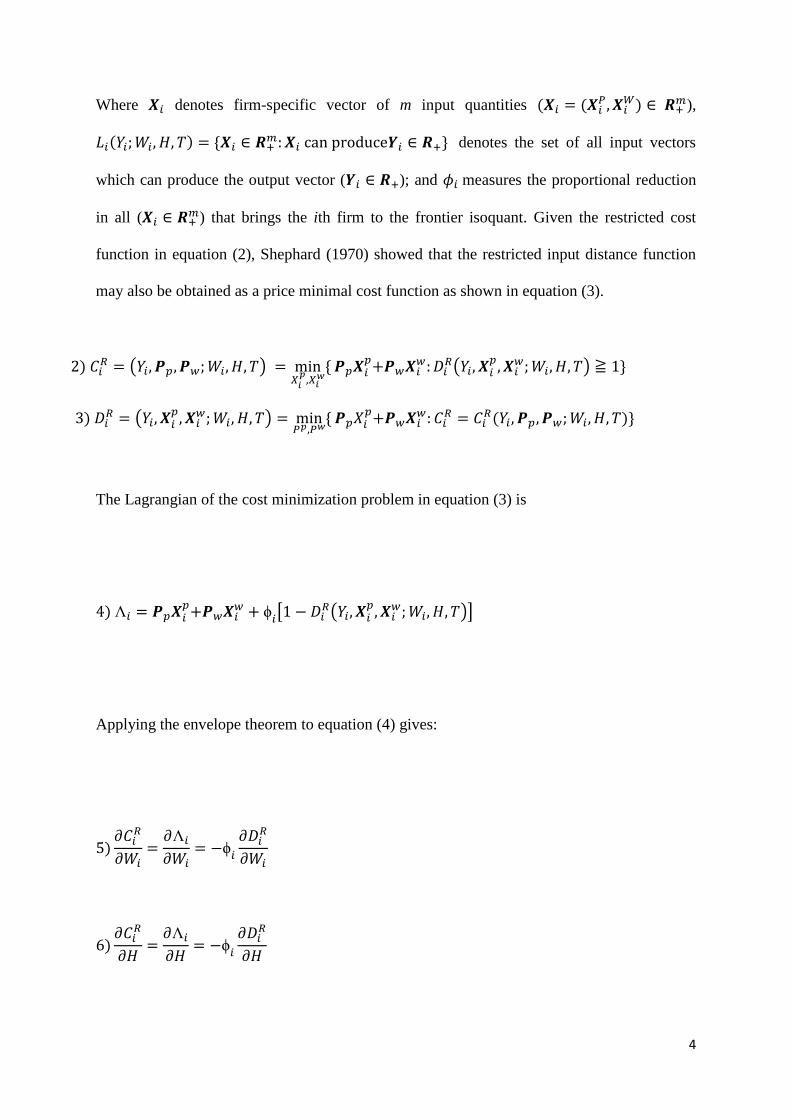
Where denotes firm-specific vector of m input quantities ( (

),

( denotes the set of all input vectors

which can produce the output vector ( ); and measures the proportional reduction

in all ( ) that brings the ith firm to the frontier isoquant. Given the restricted cost

function in equation (2), Shephard (1970) showed that the restricted input distance function

may also be obtained as a price minimal cost function as shown in equation (3).

( )

(

)

(

)

(

The Lagrangian of the cost minimization problem in equation (3) is

[

(

)]

Applying the envelope theorem to equation (4) gives:

5

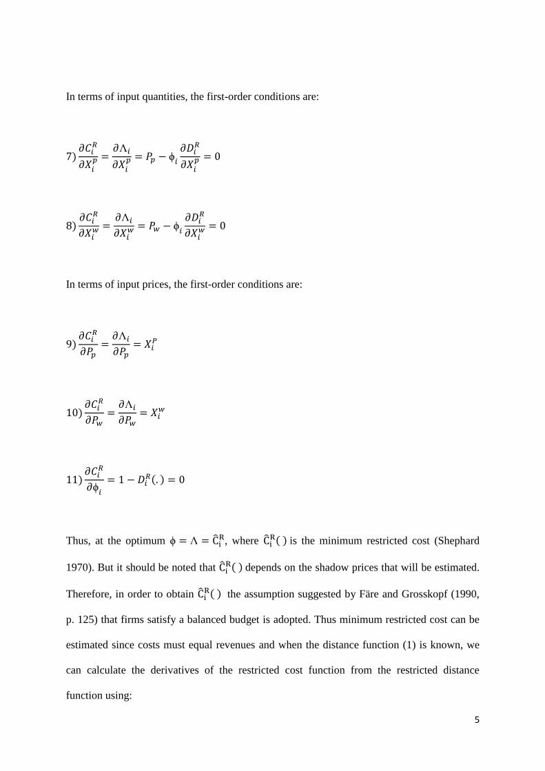
In terms of input quantities, the first-order conditions are:

In terms of input prices, the first-order conditions are:

(

Thus, at the optimum ̂ , where ̂

( is the minimum restricted cost (Shephard

1970). But it should be noted that ̂ ( depends on the shadow prices that will be estimated.

Therefore, in order to obtain ̂ ( the assumption suggested by Färe and Grosskopf (1990,

p. 125) that firms satisfy a balanced budget is adopted. Thus minimum restricted cost can be

estimated since costs must equal revenues and when the distance function (1) is known, we

can calculate the derivatives of the restricted cost function from the restricted distance

function using:

6

(

) ( ̂

)

(

) ( ̂

)

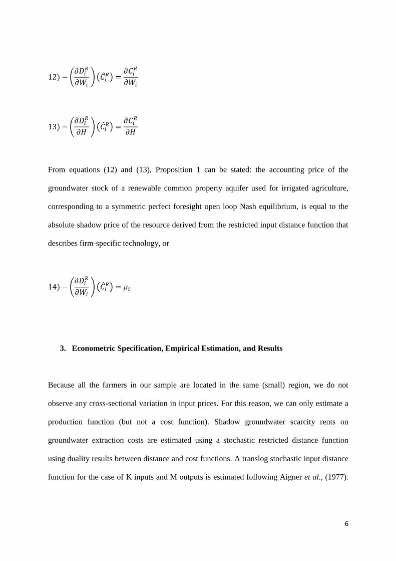
From equations (12) and (13), Proposition 1 can be stated: the accounting price of the

groundwater stock of a renewable common property aquifer used for irrigated agriculture,

corresponding to a symmetric perfect foresight open loop Nash equilibrium, is equal to the

absolute shadow price of the resource derived from the restricted input distance function that

describes firm-specific technology, or

(

) ( ̂

)

3. Econometric Specification, Empirical Estimation, and Results

Because all the farmers in our sample are located in the same (small) region, we do not

observe any cross-sectional variation in input prices. For this reason, we can only estimate a

production function (but not a cost function). Shadow groundwater scarcity rents on

groundwater extraction costs are estimated using a stochastic restricted distance function

using duality results between distance and cost functions. A translog stochastic input distance

function for the case of K inputs and M outputs is estimated following Aigner et al., (1977).

7

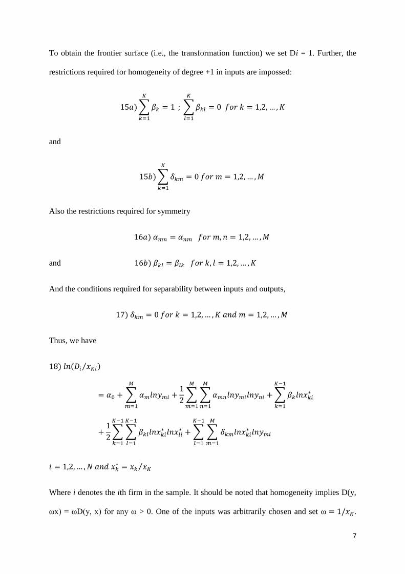
To obtain the frontier surface (i.e., the transformation function) we set Di = 1. Further, the

restrictions required for homogeneity of degree +1 in inputs are impossed:

∑

∑

and

∑

Also the restrictions required for symmetry

and

And the conditions required for separability between inputs and outputs,

Thus, we have

( ⁄

∑

∑ ∑

∑

∑ ∑

∑ ∑

⁄

Where i denotes the ith firm in the sample. It should be noted that homogeneity implies D(y,

ωx) = ωD(y, x) for any ω > 0. One of the inputs was arbitrarily chosen and set ω .

8

Therefore D(y, ) = D(y, x) ). The frontier function has an error term with two

components. The first component is a symmetric error term (Vi) that accounts for noise,

which is assumed identically and independently distributed with zero mean and constant

variance [ ( ]. The second component is an asymmetric error term (Ui) that

accounts for technical inefficiency, which is assumed to follow an iid distribution truncated at

zero (N(v, )).The two components of the error term, Vi and Ui, are independent.

Predictions for Di = exp(Ui) are obtained using the conditional expectation Di =

E[exp(Ui)|Ωi], where Ωi = Vi-Ui. Changing notation ln(Di) to Ui, equation (18) becomes:

( (

)

Equation (19) is estimated by maximum likelihood. Results are presented in Table 1. Data are

drawn from a production surveys conducted in the agricultural region close to the Asopos

River Basin in 2009. Farm-specific data includes: area of holding, land use and tenure, area

planted, production of temporary and permanent crops, production inputs (including extracted

groundwater), administrative costs, personal characteristics of buyers and sellers,

employment of holders and family members, labour costs, value of construction works and

other investments, indirect taxes and other expenses. The quality of the data-set is limited by

the usual difficulties that one encounters when attempting to document inputs and outputs of

agricultural activities. Particular difficulties where encountered in the collection of accurate

groundwater extraction rates. The data-set has 301 cross sections. The following variables

were used:

Output:

y = firm-specific total value of output from production of agricultural crops, measured in

Euros and deflated by the wholesale agricultural index.

9

Inputs:

x1 = farm-specific total area of non-irrigated land (acres),

x2 = farm-specific annual labour costs (Euros),

x3 = farm-specific total value of input costs, including fertilizers, manure, pesticides, fuel and

electric power for groundwater extraction (Euros),

x4 = farm-specific yearly groundwater extraction (m3),

x5 = farm-specific total area of irrigated land (acres); the negative of x5 is the dependent

variable of the estimated stochastic frontier.

Table 1: Estimated Parameters for the Input Distance Functiona

Variable Parameter

ML

estimates

standard-

error

t-ratiob

Constant α0 1.48E+00 1.03E+00 1.44E+00

Value of output α1 -3.96E-01 1.49E-01 -2.65E+00

Non irrigated land β1 6.14E-01 2.32E-01 2.65E+00

Labour costs β2 8.65E-02 7.26E-02 1.19E+00

Inputs costs β3 2.81E-02 1.15E-01 2.45E-01

Groundwater extraction β4 3.89E-01 1.04E-01 3.73E+00

0.5 Squared Value of Output β5 3.15E-02 1.21E-02 2.62E+00

0.5 Squared Non Irrigated land β6 -2.98E-01 3.49E-02 -8.55E+00

0.5 Squared Value of labour costs β7 2.79E-03 4.14E-03 6.75E-01

0.5 Squared inputs costs β8 -6.05E-03 1.42E-02 -4.25E-01

0.5 Squared groundwater extraction β9 -1.43E-01 8.60E-03 -1.66E+01

Value of output * Non irrigated

land

β10

1.43E-02 1.40E-02 1.02E+00

10

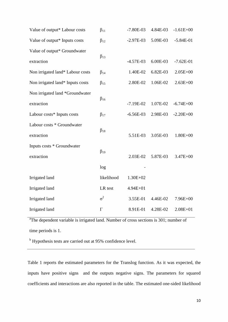
Value of output* Labour costs β11 -7.80E-03 4.84E-03 -1.61E+00

Value of output* Inputs costs β12 -2.97E-03 5.09E-03 -5.84E-01

Value of output* Groundwater

extraction

β13

-4.57E-03 6.00E-03 -7.62E-01

Non irrigated land* Labour costs β14 1.40E-02 6.82E-03 2.05E+00

Non irrigated land* Inputs costs β15 2.80E-02 1.06E-02 2.63E+00

Non irrigated land *Groundwater

extraction

β16

-7.19E-02 1.07E-02 -6.74E+00

Labour costs* Inputs costs β17 -6.56E-03 2.98E-03 -2.20E+00

Labour costs * Groundwater

extraction

β18

5.51E-03 3.05E-03 1.80E+00

Inputs costs * Groundwater

extraction

β19

2.03E-02 5.87E-03 3.47E+00

Irrigated land

log

likelihood

-

1.30E+02

Irrigated land LR test 4.94E+01

Irrigated land σ2 3.55E-01 4.46E-02 7.96E+00

Irrigated land Γ 8.91E-01 4.28E-02 2.08E+01

aThe dependent variable is irrigated land. Number of cross sections is 301; number of

time periods is 1.

b Hypothesis tests are carried out at 95% confidence level.

Table 1 reports the estimated parameters for the Translog function. As it was expected, the

inputs have positive signs and the outputs negative signs. The parameters for squared

coefficients and interactions are also reported in the table. The estimated one-sided likelihood

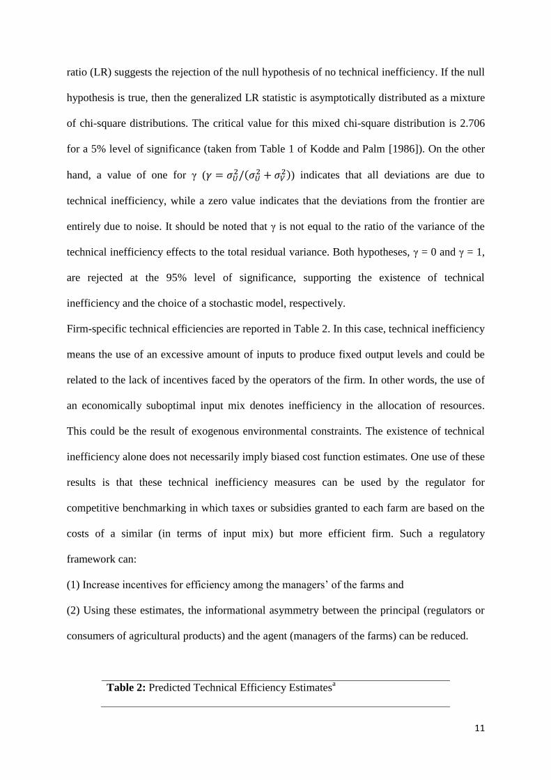
11

ratio (LR) suggests the rejection of the null hypothesis of no technical inefficiency. If the null

hypothesis is true, then the generalized LR statistic is asymptotically distributed as a mixture

of chi-square distributions. The critical value for this mixed chi-square distribution is 2.706

for a 5% level of significance (taken from Table 1 of Kodde and Palm [1986]). On the other

hand, a value of one for γ ( (

) indicates that all deviations are due to

technical inefficiency, while a zero value indicates that the deviations from the frontier are

entirely due to noise. It should be noted that γ is not equal to the ratio of the variance of the

technical inefficiency effects to the total residual variance. Both hypotheses, γ = 0 and γ = 1,

are rejected at the 95% level of significance, supporting the existence of technical

inefficiency and the choice of a stochastic model, respectively.

Firm-specific technical efficiencies are reported in Table 2. In this case, technical inefficiency

means the use of an excessive amount of inputs to produce fixed output levels and could be

related to the lack of incentives faced by the operators of the firm. In other words, the use of

an economically suboptimal input mix denotes inefficiency in the allocation of resources.

This could be the result of exogenous environmental constraints. The existence of technical

inefficiency alone does not necessarily imply biased cost function estimates. One use of these

results is that these technical inefficiency measures can be used by the regulator for

competitive benchmarking in which taxes or subsidies granted to each farm are based on the

costs of a similar (in terms of input mix) but more efficient firm. Such a regulatory

framework can:

(1) Increase incentives for efficiency among the managers’ of the farms and

(2) Using these estimates, the informational asymmetry between the principal (regulators or

consumers of agricultural products) and the agent (managers of the farms) can be reduced.

Table 2: Predicted Technical Efficiency Estimatesa

12

Firm 1-50

Firm 51-

100

Firm

101-150

Firm

151-200

Firm 201-

250

Firm 251-

301

8.38E-01 6.95E-01 7.18E-01 5.82E-01 7.07E-01 8.22E-01

7.52E-01 7.70E-01 7.85E-01 6.60E-01 7.38E-01 7.69E-01

9.50E-01 8.78E-01 7.85E-01 7.48E-01 7.55E-01 8.51E-01

7.84E-01 3.16E-01 6.48E-01 7.09E-01 7.27E-01 4.67E-01

8.28E-01 6.93E-01 7.28E-01 7.01E-01 5.04E-01 9.03E-01

8.87E-01 3.76E-01 7.23E-01 8.57E-01 6.42E-01 8.35E-01

7.50E-01 8.02E-01 7.59E-01 6.55E-01 7.49E-01 8.88E-01

8.18E-01 7.62E-01 7.10E-01 7.45E-01 7.18E-01 2.30E-01

8.41E-01 7.38E-01 7.85E-01 7.24E-01 7.14E-01 6.37E-01

6.23E-01 8.00E-01 7.41E-01 7.06E-01 7.10E-01 6.05E-01

7.43E-01 8.27E-01 7.07E-01 6.87E-01 5.76E-01 7.46E-01

8.59E-01 7.33E-01 8.23E-01 6.99E-01 8.04E-01 7.49E-01

4.84E-01 7.45E-01 7.73E-01 7.18E-01 6.80E-01 7.74E-01

7.60E-01 7.32E-01 7.46E-01 7.31E-01 6.60E-01 7.91E-01

9.05E-01 6.99E-01 7.70E-01 7.00E-01 2.69E-01 8.01E-01

6.94E-01 6.96E-01 6.48E-01 7.29E-01 2.48E-01 3.93E-01

7.45E-01 7.79E-01 6.49E-01 6.97E-01 2.56E-01 7.99E-01

8.61E-01 7.60E-01 7.48E-01 7.44E-01 7.37E-01 8.85E-01

8.79E-01 8.90E-01 6.89E-01 7.02E-01 7.40E-01 7.19E-01

8.48E-01 8.13E-01 7.15E-01 7.72E-01 6.91E-01 9.34E-01

7.08E-01 6.41E-01 6.94E-01 6.98E-01 6.91E-01 7.78E-01

7.01E-01 7.50E-01 8.27E-01 7.81E-01 9.00E-01 8.18E-01

7.37E-01 4.10E-01 6.74E-01 7.75E-01 6.78E-01 8.26E-01

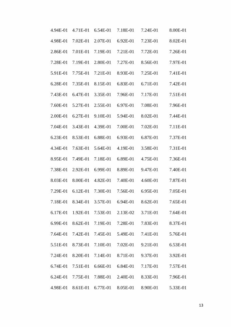
13

4.94E-01 4.71E-01 6.54E-01 7.18E-01 7.24E-01 8.00E-01

4.98E-01 7.02E-01 2.07E-01 6.92E-01 7.23E-01 8.02E-01

2.86E-01 7.01E-01 7.19E-01 7.21E-01 7.72E-01 7.26E-01

7.28E-01 7.19E-01 2.80E-01 7.27E-01 8.56E-01 7.97E-01

5.91E-01 7.75E-01 7.21E-01 8.93E-01 7.25E-01 7.41E-01

6.28E-01 7.35E-01 8.15E-01 6.83E-01 6.71E-01 7.42E-01

7.43E-01 6.47E-01 3.35E-01 7.96E-01 7.17E-01 7.51E-01

7.60E-01 5.27E-01 2.55E-01 6.97E-01 7.08E-01 7.96E-01

2.00E-01 6.27E-01 9.10E-01 5.94E-01 8.02E-01 7.44E-01

7.04E-01 3.43E-01 4.39E-01 7.00E-01 7.02E-01 7.11E-01

6.23E-01 8.53E-01 6.88E-01 6.93E-01 6.87E-01 7.37E-01

4.34E-01 7.63E-01 5.64E-01 4.19E-01 3.58E-01 7.31E-01

8.95E-01 7.49E-01 7.18E-01 6.89E-01 4.75E-01 7.36E-01

7.38E-01 2.92E-01 6.99E-01 8.89E-01 9.47E-01 7.40E-01

8.03E-01 8.00E-01 4.82E-01 7.40E-01 4.60E-01 7.87E-01

7.29E-01 6.12E-01 7.30E-01 7.56E-01 6.95E-01 7.05E-01

7.18E-01 8.34E-01 3.57E-01 6.94E-01 8.62E-01 7.65E-01

6.17E-01 1.92E-01 7.53E-01 2.13E-02 3.71E-01 7.64E-01

6.99E-01 8.62E-01 7.19E-01 7.28E-01 7.83E-01 8.37E-01

7.64E-01 7.42E-01 7.45E-01 5.49E-01 7.41E-01 5.76E-01

5.51E-01 8.73E-01 7.10E-01 7.02E-01 9.21E-01 6.53E-01

7.24E-01 8.20E-01 7.14E-01 8.71E-01 9.37E-01 3.92E-01

6.74E-01 7.51E-01 6.66E-01 6.84E-01 7.17E-01 7.57E-01

6.24E-01 7.75E-01 7.88E-01 2.40E-01 8.33E-01 7.96E-01

4.98E-01 8.61E-01 6.77E-01 8.05E-01 8.90E-01 5.33E-01

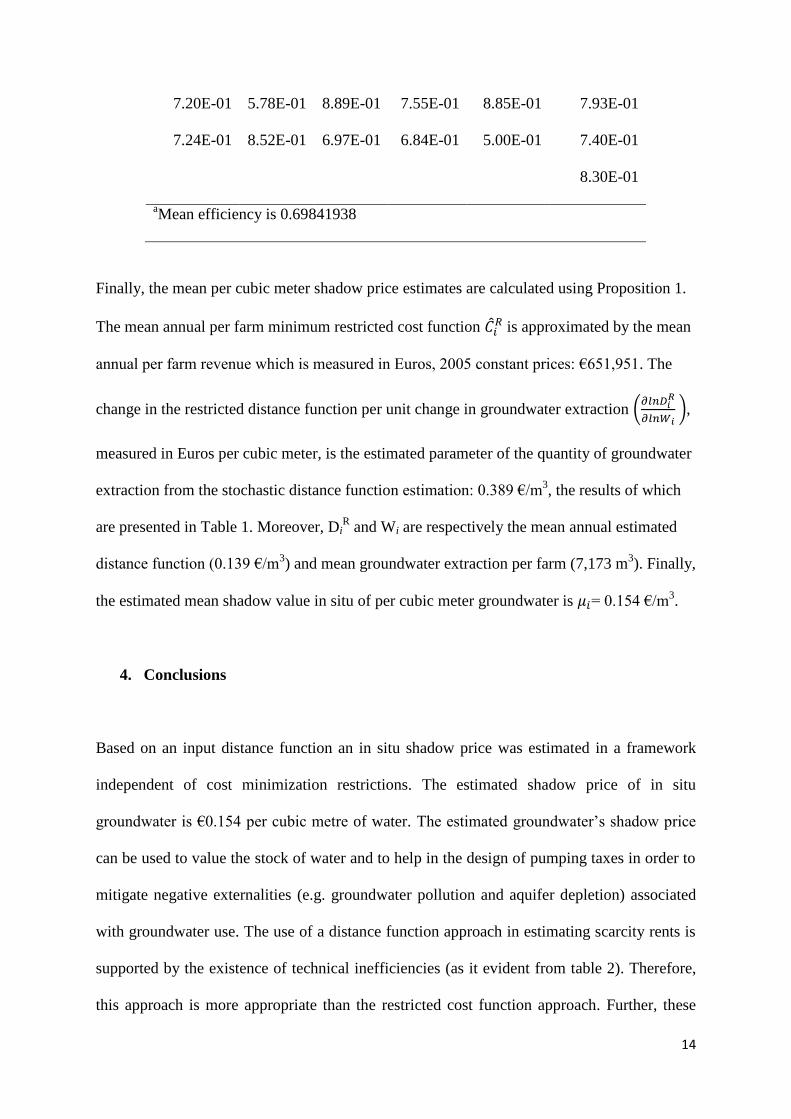
14

7.20E-01 5.78E-01 8.89E-01 7.55E-01 8.85E-01 7.93E-01

7.24E-01 8.52E-01 6.97E-01 6.84E-01 5.00E-01 7.40E-01

8.30E-01

aMean efficiency is 0.69841938

Finally, the mean per cubic meter shadow price estimates are calculated using Proposition 1.

The mean annual per farm minimum restricted cost function ̂ is approximated by the mean

annual per farm revenue which is measured in Euros, 2005 constant prices: €651,951. The

change in the restricted distance function per unit change in groundwater extraction (

),

measured in Euros per cubic meter, is the estimated parameter of the quantity of groundwater

extraction from the stochastic distance function estimation: 0.389 €/m3, the results of which

are presented in Table 1. Moreover, DiR and Wi are respectively the mean annual estimated

distance function (0.139 €/m3) and mean groundwater extraction per farm (7,173 m

3). Finally,

the estimated mean shadow value in situ of per cubic meter groundwater is = 0.154 €/m3.

4. Conclusions

Based on an input distance function an in situ shadow price was estimated in a framework

independent of cost minimization restrictions. The estimated shadow price of in situ

groundwater is €0.154 per cubic metre of water. The estimated groundwater’s shadow price

can be used to value the stock of water and to help in the design of pumping taxes in order to

mitigate negative externalities (e.g. groundwater pollution and aquifer depletion) associated

with groundwater use. The use of a distance function approach in estimating scarcity rents is

supported by the existence of technical inefficiencies (as it evident from table 2). Therefore,

this approach is more appropriate than the restricted cost function approach. Further, these

15

technical inefficiency measures can be used by the regulator. In this case, taxes or subsidies

could be granted to each farm based on the costs of a similar (in terms of input mix) but more

efficient firm. This kind of policy can increase the incentives towards efficiency, a

challenging task when regulation of common property resources is done. Besides, this could

reduce the information asymmetry between farmers, consumer and regulators, which is

another major issue for the implementation of agricultural policies.

References

Aigner, D., C. A. K. Lovell, and P. J. Schmidt (1977), Formulation and estimation of

stochastic frontier production function models, J. Econ., 6(1), 21– 37.

Coelli, T. and S. Perelman (2000), Technical efficiency of European railways: a distance

function approach, Applied Economics, 32(15), 1967-1976.

Färe, R., and S. Grosskopf (1990), A distance function approach to measuring price

efficiency, J. Public Econ., 43, 123– 126.

Färe, R., S. Grosskopf, C. A. K. Lovell, and S. Yaisawarng (1993), Derivation of shadow

prices for undesirable outputs: A distance function approach, Rev. Econ. Stat., 75(2), 374–

380.

Färe, R., S. Grosskopf, and C. A. K. Lovell (1994), Production Frontiers, Cambridge Univ.

Press, New York.

Färe, R., and D. Primont (1995), Multi-output Production and Duality Theory and

Applications, Kluwer Acad., Norwell, Mass.

16

Grosskopf, S., and K. Hayes (1993), Local public sector bureaucrats and their input choices,

J. Urban Econ., 33, 151– 166.

Howe, C. (2002), Policy issues and institutional impediments in the management of ground

water: Lessons from case studies, Environ. Dev. Econ., 7, 625– 642.

Koundouri, P. (2000), Three approaches to measuring natural resource scarcity: Theory and

application to groundwater, Ph.D. thesis, Fac. of Econ. and Polit., Univ. of Cambridge,

Cambridge, U. K.

Koundouri, P., & Xepapadeas, A. (2004). Estimating accounting prices for common pool

natural resources: A distance function approach. Water resources research, 40(6),

W06S17.

Shephard, R. W. (1970), Theory of Cost and Production Functions, Princeton Univ. Press,

Princeton, N. J.

17

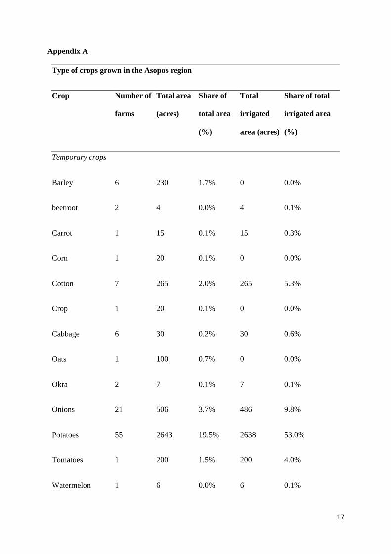
Appendix A

Type of crops grown in the Asopos region

Crop Number of

farms

Total area

(acres)

Share of

total area

(%)

Total

irrigated

area (acres)

Share of total

irrigated area

(%)

Temporary crops

Barley 6 230 1.7% 0 0.0%

beetroot 2 4 0.0% 4 0.1%

Carrot 1 15 0.1% 15 0.3%

Corn 1 20 0.1% 0 0.0%

Cotton 7 265 2.0% 265 5.3%

Crop 1 20 0.1% 0 0.0%

Cabbage 6 30 0.2% 30 0.6%

Oats 1 100 0.7% 0 0.0%

Okra 2 7 0.1% 7 0.1%

Onions 21 506 3.7% 486 9.8%

Potatoes 55 2643 19.5% 2638 53.0%

Tomatoes 1 200 1.5% 200 4.0%

Watermelon 1 6 0.0% 6 0.1%

18

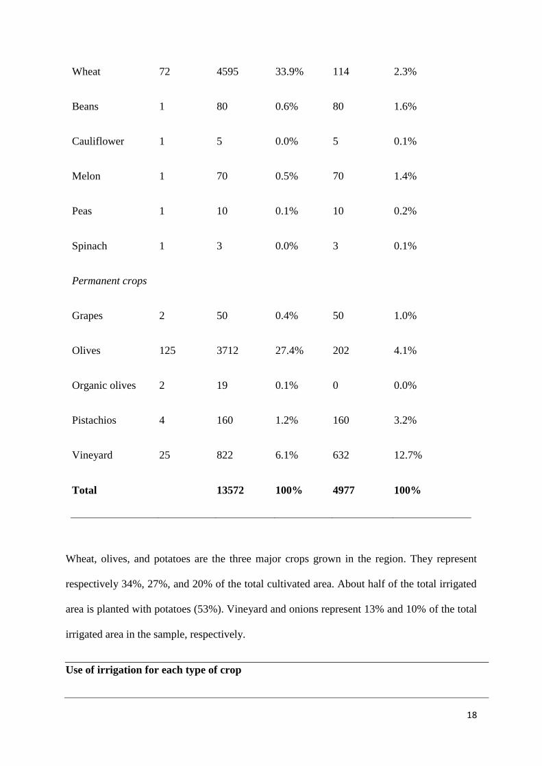
Wheat 72 4595 33.9% 114 2.3%

Beans 1 80 0.6% 80 1.6%

Cauliflower 1 5 0.0% 5 0.1%

Melon 1 70 0.5% 70 1.4%

Peas 1 10 0.1% 10 0.2%

Spinach 1 3 0.0% 3 0.1%

Permanent crops

Grapes 2 50 0.4% 50 1.0%

Olives 125 3712 27.4% 202 4.1%

Organic olives 2 19 0.1% 0 0.0%

Pistachios 4 160 1.2% 160 3.2%

Vineyard 25 822 6.1% 632 12.7%

Total 13572 100% 4977 100%

Wheat, olives, and potatoes are the three major crops grown in the region. They represent

respectively 34%, 27%, and 20% of the total cultivated area. About half of the total irrigated

area is planted with potatoes (53%). Vineyard and onions represent 13% and 10% of the total

irrigated area in the sample, respectively.

Use of irrigation for each type of crop

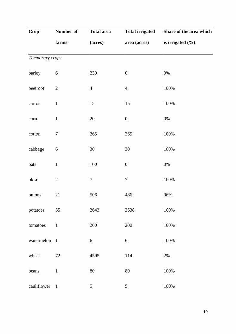
19

Crop Number of

farms

Total area

(acres)

Total irrigated

area (acres)

Share of the area which

is irrigated (%)

Temporary crops

barley 6 230 0 0%

beetroot 2 4 4 100%

carrot 1 15 15 100%

corn 1 20 0 0%

cotton 7 265 265 100%

cabbage 6 30 30 100%

oats 1 100 0 0%

okra 2 7 7 100%

onions 21 506 486 96%

potatoes 55 2643 2638 100%

tomatoes 1 200 200 100%

watermelon 1 6 6 100%

wheat 72 4595 114 2%

beans 1 80 80 100%

cauliflower 1 5 5 100%

20

melon 1 70 70 100%

peas 1 10 10 100%

spinach 1 3 3 100%

Permanent crops

grapes 2 50 50 100%

olives 125 3712 202 5%

organic

olives 2 19 0 0%

pistachios 4 160 160 100%

vineyard 25 822 632 77%

Total 340 13572 4977 37%

Cereals (barley, corn, oats, wheat) are not irrigated in general. Only 5% of the area planted

with olive trees is irrigated. Fields planted with cotton, fruits, and vegetables are fully

irrigated. Overall, 37% of the total area in the sample is irrigated. The three major products

that are grown in Asopos are wheat, olives, and potatoes. We can see from this table that

farmers do not combine wheat, olives, or potatoes with the growing of other products in most

cases.

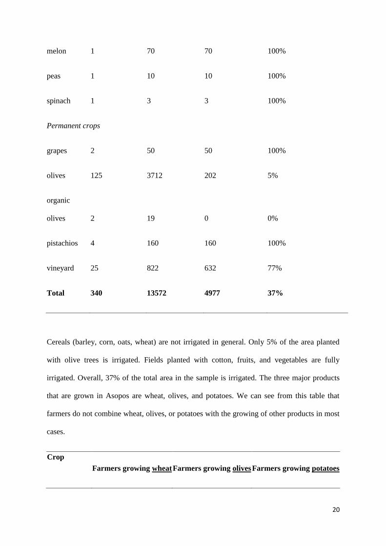
Crop

Farmers growing wheat Farmers growing olives Farmers growing potatoes

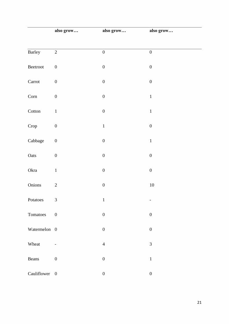
21

also grow… also grow… also grow…

Barley 2 0 0

Beetroot 0 0 0

Carrot 0 0 0

Corn 0 0 1

Cotton 1 0 1

Crop 0 1 0

Cabbage 0 0 1

Oats 0 0 0

Okra 1 0 0

Onions 2 0 10

Potatoes 3 1 -

Tomatoes 0 0 0

Watermelon 0 0 0

Wheat - 4 3

Beans 0 0 1

Cauliflower 0 0 0

22

Melon 0 0 1

Peas 0 0 0

Spinach 0 0 0

Grapes 0 0 0

Olives 4 - 1

Organic

olives 0 0 0

Pistachios 0 0 0

Vineyard 0 1 2

The three major crops in the area are wheat, potatoes and olives, which we will consider in

turn.

Wheat producers

In what follows we consider the 59 farmers who grow only wheat (overall 72 farmers grow

wheat in our sample). The following inputs are considered: fertilizers, pesticides and labour.

Fertilizers and pesticides use are farmers’ statements while labour is calculated as follows:

number of days of casual workers + number of permanent workers x 250. Some basic

statistics are shown below. There are all on a per acre basis.

Variable Obs. Mean Std. Dev. Min Max

23

Production (tonnes/acre) 59 0.27 0.19 0.02 0.80

Fertilizer use (kg/ acre) 58 17.07 15.37 0.00 60.00

Pesticides use (kg/ acre) 55 0.27 0.60 0.00 2.14

Labour use (days/acre) 59 0.15 0.27 0.00 1.50

Land (acre) 59 70.61 85.86 6.00 500.00

All these statistics are on a per acre basis so the figures should not vary too much from one

farmer to the other. However we observe very large variations. For example, fertilizer use

varies from 0kg/acre to 60kg/acre, with a mean of 17kg/acre. The farmers stating 0 use of

fertilizer, pesticides or labour probably did not want to answer or did not know. For these

farmers, I have replaced 0 by the median value in the sample of farmers growing wheat only.

Statistics on yield

1 Acre - US, = 0.4046873 ha, 1 hectare (ha), = 2.471044 acre (US)

Farmers in the sample produce on average 0.27 tonnes per acre, which corresponds to 0.67

tonnes per hectare (or 670kg per ha). The average wheat yield in Greece is 1900 – 3000

kg/ha. The average yield on the sample thus seems a bit low. Once all variables are

transformed in logs a Cobb Douglas production function is estimated. Because of the small

sample size, it is not reasonable to estimate a Translog production function.

24

OLS estimation results – Cobb Douglas production function (59 obs)

Coef. Std. Err. P>t

Fertilizer 0.026 0.093 0.778

Pesticides 0.204 0.119 0.092

Labour 0.140 0.080 0.087

Constant -0.127 0.146 0.386

In this model the dependent variable is wheat yield. The explanatory factors are the three

inputs measured in physical terms: fertilizer use per acre, pesticides use per acre, labour use

per acre. The three estimated coefficients have the expected positive sign but only two are

significant at the 10% level. However, the model is not significant overall (p-value of the

Fisher test is 0.1251). As a consequence the adjusted R-squared is also quite low: 0.0491.

Potatoes producers

In what follows we consider the 34 farmers who grow only potatoes (overall 55 farmers grow

potatoes in our sample). Some basic statistics are shown below.

Variable Obs Mean Std. Dev. Min Max

Production (tonnes/acre) 34 2.04 1.13 0.20 5.00

25

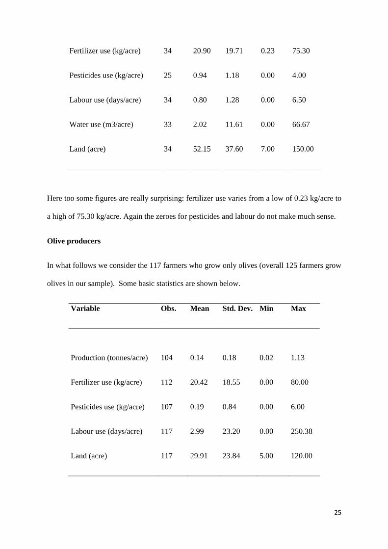
Fertilizer use (kg/acre) 34 20.90 19.71 0.23 75.30

Pesticides use (kg/acre) 25 0.94 1.18 0.00 4.00

Labour use (days/acre) 34 0.80 1.28 0.00 6.50

Water use (m3/acre) 33 2.02 11.61 0.00 66.67

Land (acre) 34 52.15 37.60 7.00 150.00

Here too some figures are really surprising: fertilizer use varies from a low of 0.23 kg/acre to

a high of 75.30 kg/acre. Again the zeroes for pesticides and labour do not make much sense.

Olive producers

In what follows we consider the 117 farmers who grow only olives (overall 125 farmers grow

olives in our sample). Some basic statistics are shown below.

Variable Obs. Mean Std. Dev. Min Max

Production (tonnes/acre) 104 0.14 0.18 0.02 1.13

Fertilizer use (kg/acre) 112 20.42 18.55 0.00 80.00

Pesticides use (kg/acre) 107 0.19 0.84 0.00 6.00

Labour use (days/acre) 117 2.99 23.20 0.00 250.38

Land (acre) 117 29.91 23.84 5.00 120.00