Chapter 5 A Simplification of Weights of Evidence using a ... · A Simplification of Weights of Evidence using a Density Function and Fuzzy Distributions; Geothermal Systems, Nevada

115

A Simplification of Weights of Evidence using a Density Functionand Fuzzy Distributions; Geothermal Systems, Nevada

Mark F. CoolbaughGreat Basin Center for Geothermal Energy, Mackay School of Mines, Department of Geological Sciences,

MS 172, University of Nevada, Reno, NV, USA, 89557-0138

Richard L. BedellArthur Brandt Laboratory for Exploration Geophysics, Mackay School of Mines, Department of Geological Sciences,

MS 172, University of Nevada, Reno, NV, USA, 89557-0138 and AuEx Ventures Inc., 940 Matley Lane, Suite 17, Reno, NV, USA, 89502

Abstract

Probability modelling in the geosciences has been dominated by binary weights-of-evidence techniques. However, thereduction of each layer of data to a binary yes or no designation is not considered adequate by all geoscientists.Alternate methods define gradational weights over a range of values, as is done with fuzzy logic modelling. The prob-lem with fuzzy logic is that there is no unbiased way to combine layers of evidence, and the relationship between fuzzyweights and probability distributions is undefined.

A new technique for estimating weights over a range of evidence values is proposed. A density function is defined as thefraction of the total training sites occurring within a given histogram bin of an evidence layer's data distribution, divid-ed by the fraction of the total study area within that bin. If the total training site area is small relative to the total studyarea, as is often the case, then the natural log of this density function approximates a weight of evidence. Evidence lay-ers represented by the density function can be added together in log-transformed space in a manner analogous to theposterior logit calculation in weights of evidence.

Using geothermal systems in Nevada, USA, as an example, the density function model correlates remarkably well withbinary weights of evidence, suggesting not only that the density method can mimic data-driven probabilistic methods,but also that binary weights of evidence is a robust technique in its own right. However, the density function methodyields more detailed favourability rankings than binary weights of evidence, potentially advantageous in "vectoring in"toward exploration targets. The density method also offers ease of calculation; minimal expert guidance is used tosmooth statistical noise that can make determination of multiclass weights of evidence difficult.

Résumé

En sciences de la Terre, le domaine de la modélisation des probabilités a été dominé par des techniques de pondérationde d'informations probantes binaires. Cependant, la réduction de chaque couche d'information en données binaire(présence ou absence) est insatisfaisante pour nombre de géoscientifiques. D'autres méthodes utilisent des échelles de

Chapter 5

INTRODUCTION

The choice of which method to use in building a predictive modeldepends, in part, on the acceptance and understanding of those thatwill use it. In reality, the model is only one component of the deci-sion-making process (Figure 1). The conceptualization of a problemis derived from human understanding, and decisions to implementa program in a legal or financial context (usually both) involveindividuals. In the mining industry, these individuals typicallyinclude a spectrum of managers and data experts, who must be com-fortable with the data going in and how it is represented in themodel.

Individual experts must be convinced that the data layers theyare most familiar with are adequately represented in the model. Inthe authors' experiences working with surveys, academics, and min-ing companies, acceptance of binary input is difficult for some dataspecialists. Although binary patterns can work well, as in the exam-ple of distinguishing between anomalous and background values ingeochemistry (Bonham-Carter et al., 1988), some experts prefermore continuous data distributions that more intuitively and quanti-tatively represent the data. In contrast, managers are often moreconcerned with understanding the entire modelling method, espe-cially if the modelling results do not fit preconceived notions.Therefore, for acceptance in a larger decision-making context, it isadvantageous for the modelling process to be as simple as possible,and advantageous for the model to fully represent data distributions.Much previous modelling using Geographic Information Systems(GIS) has invoked simple Boolean overlay of evidence and additionof evidence layers, with or without an additional expert weighting(Pan and Harris, 2000; Drury, 1993). These methods, although over-ly simplistic, are intuitive and allow a consensus in the decisionmaking process. These methods do not consider the essential con-cepts of prior and posterior probability which are central toBayesian methods.

Binary weights of evidence (WofE) offers a more rigorous andobjective statistical approach that has found many applications inmodelling real world situations (Agterberg, 1989; Bonham-Carter,1996; Knox-Robinson, 2000; Raines and Bonham-Carter, this vol-ume; Mihalasky, this volume). A major benefit of WofE is the unbi-ased, statistically derived weight it provides for individual layers ofdata (evidence maps). However, WofE is perceived by some usersas both an oversimplification because of its typically binary input,and yet overly complex in mathematics. Multiclass WofE offers bet-

116

GIS FOR THE EARTH SCIENCES

pondération appliquée à une gamme de valeurs, comme c'est le cas dans la modélisation par logique floue. Le problèmeavec les méthodes par logique floue, c'est qu'il n'existe pas de façon impartiale de combiner les couches d'information,et que la relation entre les pondérations floues et les distributions de probabilités sont non-définies.

Une nouvelle technique d'estimation de la pondération par gamme d'indices est proposée. Une fonction de densité estdéfinie comme étant la fraction du nombre total de sites de référence de la population des classes d'un histogramme dela distribution des indices d'une couche d'information probante, divisée par la fraction de la surface totale étudiée cor-respondant à cette population. Si la surface de tous les sites de référence est petite par rapport à la surface de la zoneétudiée, comme c'est souvent le cas, alors le log naturel de cette fonction de densité équivaut à peu près à la pondéra-tion de l'information probante. Les couches d'indices représentées par la fonction de densité peuvent alors être addition-nées dans un espace transformé logarithmiquement, comme on le ferait dans un calcul logit a posteriori d'une pondéra-tion d'information probante.

En prenant des systèmes géothermaux dans l'État de Nevada aux États-Unis comme exemples, la fonction de densitéaffiche une remarquable corrélation avec la pondération d'information probante binaire, permettant de croire non seule-ment que la méthode par fonction de densité peut reproduire les résultats de méthodes probabilistes à base de données,mais aussi que la méthode binaire par pondération d'information probante est elle-même une technique robuste. Celadit, la méthode par fonction de densité produit donne des niveaux de favorabilité plus nombreux que la méthode binairede pondération d'information probante, ce qui peut s'avérer intéressant au moment d'établir des cibles d'exploration parvectorisation. La méthode par fonction de densité présente l'avantage d'un calcul facile et ne requiert une assistanceexperte que pour lisser le bruit de fond statistique, dans les cas où il s'avérerait difficile de déterminer une pondérationde l'information probante multiclasse.

Figure 1. Probability modelling is a component of decision-making.Individuals derive the exploration concept based on their interac-tion with the data and the probability model. The decision to pro-ceed is a management decision and managers need to grasp themodelling concept. The manager in turn is influenced on an individ-ual level by data experts who will argue against an over-simplifica-tion of their data as a binary input layer.

SPECIAL PUBLICATION 44

117

ter representation of data distributions, but statistical noise cansometimes limit the effective use of multiclass weights.

Fuzzy logic methods offer gradational weighting schemes forindividual data layers and relatively simple arithmetic operationsfor combining evidence layers into predictive models. With fuzzylogic, when data layers are assembled, it is done with the opinion ofan expert. Expert input helps ensure the appropriate use of data, butthe advantages of unbiased statistical weighting are lost. Bedell(2000) recently presented an unbiased method of combining fuzzymembership functions from diverse evidence layers using geother-mal systems as an example. His weighting scheme is based on com-paring the cumulative frequency distribution of a data layer to thedata layer intersected with training points (mineral deposits oroccurrences). An F-Factor was used for normalizing areas under thecumulative frequency curves to compare the original data with thatintersecting the known geothermal systems. This method minimizesexpert bias, but the weights are not derived in a formal probabilis-tic context.

Few examples are available where researchers have mergedthe statistical rigor of WofE with the gradational weighting schemesafforded by fuzzy logic. One example is provided by Cheng andAgterberg (1999), who proposed a "fuzzy weights of evidence"method in which membership functions are scaled to cumulativecontrast. In this paper, we present a "density function" method thatis similar to the approach of Cheng and Agterberg (1999) in that itprovides a multiple-class weighting scheme for evidence layers.This new technique emphasizes simplicity of calculation and inter-pretation, and although the method strictly speaking belongs to"fuzzy logic", it's predictions track closely with, and correlatestrongly with, WofE. The suggested methods are simple and there-fore can readily be accepted by group decision. They can be easilyimplemented on any GIS platform without program development.The use of multiclass weighting helps maintain the integrity anddetail of individual data distributions in the model. The objective ofthis paper is to show that a simple model using the ratios of normal-ized geothermal systems over normalized areas (a density factor)provides a robust method integrating most of the benefits of WofEand all of the benefits of fuzzy logic.

GEOTHERMAL GIS

A GIS of active geothermal systems in Nevada, USA, recently con-structed by Coolbaugh et al. (2002), was used to evaluate the den-sity function method and compare it to binary WofE. The use of thegeothermal case study provided an opportunity to explore multi-class weighting techniques for evidence layers using a diversedataset whose predictive potential had already been explored usingother techniques.

Electric power-producing geothermal systems in Nevada areunlike most others in the world because they are not closely associ-ated with young silicic volcanism (Koenig and McNitt, 1983).Instead, geothermal systems in Nevada (termed "extensional-type"geothermal systems by Wisian et al. (1999)) are associated withareas of high crustal heat flow and active extensional faulting(Koenig and McNitt, 1983; Wisian et al., 1999).

Many disparate types of evidence can help signal the locationof an "extensional-type" system, making this problem well suited

for statistical analysis within a GIS. In this study, seven evidencelayers were used. A brief description of each evidence layer follows;further discussion can be found in Coolbaugh et al. (2002).Geothermal training sites are also discussed below.

Regional Heat Flux

Geothermal systems are known to correlate with regions of highheat flux (Sass et al., 1971; Wisian et al., 1999). High heat flowbrings more thermal energy close to the earth's surface where it canheat circulating meteoric fluids. A regional digital heat flow mapwas provided by David Blackwell of Southern MethodistUniversity (SMU). Blackwell (1983) discusses some of the meth-ods and considerations used to construct the heat flow map; thatmap and further discussions are posted at the SMU geothermalwebsite located at http://www.smu.edu/geothermal/.

Young Faults

In Nevada and elsewhere in the world, geothermal systems are asso-ciated with areas of active faulting (Koenig and McNitt, 1983;Wisian et al., 1999; Bowen, 1989) because fault and fracture sys-tems are the principal means by which meteoric fluids penetratedeeply into the crust. Also in Nevada, northeast-trending youngfaults are more closely associated with high-temperature geother-mal activity than northwest-trending young faults, a relationshipdescribed earlier by Rowan and Wetlaufer (1981) and Koenig andMcNitt (1983) and confirmed by Coolbaugh et al. (2002) using spa-tial statistics. This, in turn, has been linked to extensional crustalstrain in Nevada (Blewitt et al., 2002; Coolbaugh et al., 2002),which for much of the state is directed northwesterly (as determinedby a strain net measured by GPS stations (Bennett et al., 1998)). Forthe current analysis, a map of late Pleistocene and younger faultsproduced by Dohrenwend et al. (1996), and assembled into a digi-tal database by Raines et al. (1996), was used. A buffered mapshowing the distance to the nearest northeast-trending young faultwas created for input into the model.

Depth to Water Table

The depth to the water table can be considered as the geothermalequivalent of "outcrop" in mineral exploration. Hot springs aremore likely to occur where the depth to the water table is shallow(Koenig and McNitt, 1983). Subsurface geothermal systems aremore likely to be discovered in areas where hot springs are presentat the surface. This is believed to be the reason why deep watertables negatively correlate with known geothermal systems inNevada (Coolbaugh et al., 2002). Future exploration in areas withdeeper water tables might locate more geothermal systems. A mapof depth to the water table was generated using water well informa-tion from the United States Geological Survey (USGS) NationalWater Information System (NWIS) database (http://waterdata.usgs.gov/nv/nwis/gwlevels).

Groundwater Geochemistry

Geothermal fluids often contain high concentrations of certain met-als, including boron, lithium, and arsenic (Ellis and Mahon, 1977;White et al., 1976; Ballantyne and Moore, 1988) compared to mostgroundwater. Anomalous concentrations of these metals in ground-

water can therefore be an indicator of geothermal activity. Boronconcentrations in groundwater were found by Coolbaugh et al.,(2002) to correlate best with geothermal activity in Nevada com-pared to other dissolved metals; consequently a map of groundwa-ter boron concentrations (derived from the NWIS database) wasused as a predictive (evidence) layer in the model.

Young Volcanics

Even though extensional geothermal systems in Nevada are notdirectly related to active volcanism, volcanic rocks 1.5 Ma oryounger (mostly mafic in composition) are preferentially associatedwith geothermal activity in the state (Coolbaugh et al., 2002). Twopossible explanations for this correlation are: 1) recent volcanism isrestricted to areas of active crustal extension where hydrothermalfluids might circulate to greater depth, and 2) if sufficiently young,the volcanic rocks may indicate areas of high heat-flow at depth. Anage-date database compiled by Mark Mihalasky and incorporatedinto the Great Basin Digital Database (Raines et al., 1996) was usedto create a buffered map of the distance to the nearest young vol-canics in the state.

Earthquakes

Earthquakes reveal areas of active faulting where pathways fordeeply circulating hydrothermal fluids could be present. Maps ofearthquake density were derived by adding all earthquake magni-tudes greater than 4.0 within a radius of 40 km for each cell in themodel. A threshold magnitude of 4.0 was selected because lowermagnitude quakes may not be detected in all portions of the state asa result of limitations in the distribution of observatories (DianeDePolo, personal communication, 2001). Earthquake data weretaken from catalogues maintained by the Nevada SeismologicalLaboratory at the website http://www.seismo.unr.edu/ftp/pub/catalog/.

Paleozoic Carbonates

In Nevada, deep aquifers occur in thick sequences of Paleozoic car-bonate rocks in the eastern third of the state (Harrill and Prudic,1998). Relatively few geothermal systems having high tempera-tures are known in areas underlain by the carbonate rocks; it isbelieved that the deep aquifers trap and entrain rising thermal flu-ids, preventing them from reaching the surface where they could beobserved (Sass et al., 1971). An interpretive map of Paleozoic car-bonate rocks, partially projected beneath Cenozoic cover(Ludington et al., 1996), was obtained in digital format from TheNevada Bureau of Mines and Geology.

Training Sites

Fifty-nine geothermal systems and hot springs in Nevada comprisethe training set used for modelling. These sites represent all knownoccurrences where geothermal fluids have been measured, or areestimated to have reached, a temperature of 100°C or hotter.Temperatures were either measured directly or estimated usinggeothermometer calculations based on fluid chemical compositions(Mariner et al., 1982; Coolbaugh et al., 2002). Sources of data usedto assemble the set of training points include Garside (1994),

Shevenell et al. (2000), and a western U.S. geothermal databasemaintained at SMU (Richards and Blackwell, 2002; http://www.smu.edu/geothermal/).

WEIGHTS-OF-EVIDENCE MODEL

A binary WofE model was constructed using the same training sitesand evidence layers used to build the density function model.ArcView 3.2a software was used for modelling computations, andArc-SDM, an ArcView extension, was used for WofE calculations.Arc-SDM is a spatial data-modelling package developed by theGeological Survey of Canada (GSC) and the United StatesGeological Survey (Kemp et al., 2001).

Weights-of-evidence analysis is based on Bayes' Theorem,which assumes conditional independence between evidence maps.The application of WofE analysis to mineral deposit modelling hasbeen described previously (Bonham-Carter et al., 1988; Bonham-Carter, 1996, ch. 9; Wright, 1996) and is not discussed further here.Raines et al. (2000) and Raines and Bonham-Carter (this volume)provide a concise description of the application of WofE analysis tomineral deposit exploration using ArcView software.

For each of the seven evidence layers in the model, a binarymap was produced indicating areas favourable and unfavourable forthe occurrence of geothermal systems. The optimal binary patternfor each map was determined by either maximizing the WofEcumulative contrast statistic (C), or by maximizing the Studentizedcontrast statistic (SC, see below). The contrast is defined as theabsolute difference between positive (W+) and negative (W-)weights of evidence (Wright, 1996, p. 110; Bonham-Carter, 1996, p.253-256):

C = | W+ - W- | (1)

The Studentized contrast is a measure of confidence, and is definedas the ratio of the contrast divided by its standard deviation(Bonham-Carter, 1996, p. 323):

SC = C / Scontrast = |(W+ - W-)|/ {sqrt[s2(W+) + s2(W-)]} (2)

For evidence layers with a maximum contrast greater than 2, themaximum contrast was used to determine the binary pattern. Forevidence layers where the maximum contrast was less than 2, themaximum Studentized contrast was used instead, to help insure sta-tistical significance.

Positive weights, negative weights, contrast, and Studentizedcontrasts for each of the seven evidence layers are listed in Table 1.The unit area assigned to each geothermal system was 9 km2, whichcorresponds to the approximate average lateral dimensions of ageothermal system, based on the distribution of drillholes in well-explored systems. The study area encompasses the entire state ofNevada in the United States.

A favourability map of known geothermal systems in Nevada(Figure 2a) was made by combining the statistically-derivedweights of the seven evidence layers using a posterior logit equation(Bonham-Carter, 1996, equation 9-33). The posterior logit was cho-sen for plotting "favourability" instead of the more customary pos-terior probability, because the former yielded superior amounts ofcolour-scaled detail on the map, and was the only representation of

118



119

Table 1. Statistics for the seven evidence layers used to build the binary weights of evidence model. The columns titled “Additional Classes”list the number of additional weights potentially justified for each layer, using the arguments presented in the section on “StatisticalSignificance”

Standard Additional AdditionalPositive Negative Student Deviation Classes Classes

Evidence Layer Weight Weight Contrast Contrast of Contrast (z score = 2) (z score = 1)

Young Volcanics 2.48 -0.05 2.52 4.22 0.5989 1.1 3.2Water Table Depth 0.19 -2.22 2.41 2.39 1.0108 0.2 1.4Regional Heat Flux 0.14 -2.12 2.26 2.24 1.0087 0.1 1.2Paleozoic Carbonates 0.34 -1.42 1.77 3.78 0.4676 0.9 2.8NE-trending Young Faults 1.41 -0.11 1.52 3.99 0.3816 1.0 3.0Boron in Groundwater 0.75 -0.48 1.23 4.40 0.2787 1.2 3.4Earthquakes 0.22 -0.32 0.54 1.97 0.2753 0.0 1.0

Sum: 4.5 16.0

Figure 2a. Favourability map for geothermal systems in Nevada,based on the posterior logit of binary weights of evidence. Higherfavourabilities in northwestern Nevada are due in part to higherheat flow, presence of northeast-trending young faults, and a lack ofdeep carbonate aquifers, compared to the remainder of the state.The colour version of this figure shows background topographicshading.

Figure 2b. Favourability map of geothermal systems in Nevadabased on the density function. Because a multiclass instead of bin-ary weighting scheme was employed, more gradations in favoura-bility ranking are available compared to binary weights of evidence(Figure 2a). This helps define the Humboldt structural zone (Figure2a). The colour version of this figure shows the variations infavourability in more detail. The colour version also features back-ground topographic shading.

weights that could compete with the detailed colour-rankings pro-vided by the density function method discussed below. A possibleexplanation is provided by the fact that posterior probabilities inthis study approximate a log-normal distribution, and plotting on alog-scale (such as that afforded by the posterior logit equation)should yield a better spread of rankings. This is crudely analogousto plotting log-normal distributed geochemical data using contourintervals that progress logarithmically instead of arithmetically.

An overall conditional independence (C.I.) index of 0.76,based on the method of Bonham-Carter (Bonham-Carter, 1996, p.315), indicates some dependencies among the data and suggests thetotal number of geothermal systems is over-predicted by roughly30%. It is for this reason that the posterior probability map (Figure2a) was labelled a "favourability map" instead of a "posterior prob-ability" map. Since the primary objective of this paper was to com-pare modelling methods, conditional dependency issues were notconsidered further because they will affect both the WofE modeland the density function model (discussed below) similarly.

DENSITY FUNCTION MODEL

The density function (DF) measures the "density" or "frequency" oftraining sites (known geothermal systems) within a given map pat-tern, and is defined as the fraction of training sites falling in a givenmap pattern divided by the fraction of the study area covered by thatsame pattern:

DFi,j = [ (Ni/Nt) / (Ai/At) ]j (3)

where DFi,j = the density function value for the ith pattern on evi-dence map j, Ni = number of deposits or geothermal systems asso-ciated with pattern i, Nt = total number of deposits, Ai = area of thepattern i (on the evidence map j), and At = total area of the study. Ifa multiple number of mutually exclusive i patterns are defined for agiven evidence layer j, each pattern may have a different density oftraining points.

Defined in this manner, the area-weighted average value of thedensity function (DF) for a given evidence layer over an entirestudy area will always equal 1. Values of DF greater than 1 indicatea favourable or positive association between a pattern and the train-ing sites, while values less than one indicate an unfavourable ornegative association. If portions of the study area are lacking evi-dence (no information), a neutral value of 1 can be assigned.

When expressed in log form, values for the density functionare usually very similar to a weight of evidence. In fact, when thetotal area of training sites is small relative to the study area andsmall relative to the area of a given map pattern, the similaritybetween DF (in log form) and the weight of evidence can be demon-strated mathematically. In WofE analysis (using the nomenclatureof Bonham-Carter et al. (1988)), a positive weight can be defined asfollows:

Wj+ = ln [ P(J|D) / P(J| 9D) ] (4)

where Wj+ equals the positive weight of evidence, P(J|D) equals the

probability of map pattern j being present given a training site ispresent, and P(J| 9D) equals the probability of map pattern j beingpresent given a training site is not present. When weights aredefined for multiple classes on an evidence layer, the equation for a

positive weight (4) can be generalized so it represents all weightsfor an evidence layer, regardless of whether they are positive ornegative:

Wi,j = ln [ P(Ji|D) / P(Ji| 9D) ] (5)

where in this case Wi,j equals the weight (which could be either pos-itive or negative) for the "i"th pattern for evidence map j, P(Ji|D)equals the probability of given map pattern Ji being present given atraining site is present, and P(Ji| 9D) equals the probability of givenmap pattern Ji being present, given a training site is not present.

For the numerator of equation (5), using the definition ofP(Ji|D) it can be shown that:

P(Ji|D) = (Ni/Nt)j (6)

For the denominator, following the terminology of Bonham-Carteret al. (1988, p. 1588):

P(Ji| 9D) = [(Ai ! Adi ) / (At ! Adt )]j (7)

where Adi = the total area of deposits in pattern i and Adt = the totalarea of deposits in the study area.

When the area of a deposit is very small, both Adi and Adt arelikely to be very small relative to Ai (the total area of the pattern i)and At (the total study area). In that case:

P(Ji| 9D) = [(Ai ! Adi ) / (At ! Adt )]j =~ (Ai / At)j (8)

With substitution of equations (6) and (8), equation (5) becomes:

Wi,j =~ ln [ (Ni/Nt) / (Ai/At) ]j =~ ln (DFi,j) (9)

It is important to emphasize the simplicity of this method, given thebasic assumption. If the total spatial area of the training sites issmall (i.e., the area of active geothermal systems relative to theentire State of Nevada or relative to a given map pattern), then thelog-transformed density function can serve as a simplified proxy forweights of evidence.

Smoothed Density Function

For those layers in the geothermal model represented by real num-bers (i.e., ratio or non-categorical data), DF values were found tochange systematically over the range of data values, supporting theargument for a multiple, instead of binary, weighting scheme. As anexample, Figure 3 shows how DF increases systematically withincreasing heat flux. The higher the regional heat flux at a givenlocation in Nevada, the more likely a geothermal system (with atemperature $100°C) will occur. This relationship was previouslydocumented by Wisian et al. (1999) using a similar density calcula-tion, though they did not integrate the information with other evi-dence layers in a GIS or produce predictive maps.

Figure 3 was produced by reclassifying a real-number, interpo-lated grid map of heat flux values into a map with a finite numberof categories of progressively increasing heat flux values. Each cat-egory can be considered as a histogram bin with a correspondingunique map pattern, for which a DF value can be calculated. Notethat this is a categorical graph, not a cumulative graph. Also worthyof note is that for each of the evidence layers, WofE and densityfunction statistics proved to be nearly identical, as shown in Figure4 for the case of heat flux.

120



121

Figure 3. Density function plot for regional heat flux. Raw density function (DF) values were calculated directly from the data using equa-tion (3). Heat flux values were subdivided into 21 histograms, each with an equal spacing of 2.87 heat flux units (mWm-2): the mid-point ofeach bin was used to plot DF values. A smoothed curve was fitted to the raw DF data, and smoothed DF values were recalculated for eachhistogram bin. Some histogram bins at the low end of the heat flux scale were grouped together, so that 16 different smoothed DF valueswere used for modelling. The fraction of the total area covered by each histogram pattern is also indicated.

Figure 4. Log-transformed raw DF values compared to multiclass weights of evidence for the regional heat flux evidence layer. At the scaleof the plot, density function and weights-of-evidence statistics are virtually identical (irresolvable).

Individual DF values on Figure 3 appear erratic. This "noise"is caused by use of a large number of bins (21 total), causing a smallnumber of training points to fall into some categories. Measurementnoise could be reduced by using coarser bin spacings, but at a sac-rifice of resolution at the high flux end of the scale. Alternatively, asmooth curve could be fitted to the data using algorithms and/orexpert guidance, and in this paper for simplicity we used "expertguidance", as shown in the heat flux example (Figure 3), whereinterpretation of a steadily increasing DF is straightforward. Themethod presented here is not the only one available, and other meth-ods, such as linear regression, or bin size equalization using thenumber of training points (J. Harris, personal communication,2003) could yield equivalent results, and more research in this areais warranted. In any case, a proper balance between bin size andcurve fitting should yield optimal results.

Raw and smoothed DF values were calculated for the fiveother real-number-based evidence layers (Figures 5 to 9) used in themodelling. In each case, DF values progress from low to high val-ues as the correlative evidence either decreases, as in the case of thedepth to the water table (Figure 5), buffer distance to northeast-trending faults (Figure 6), and buffer distance to young volcanics(Figure 7), or increases, as in the case of the concentration of boronin groundwater (Figure 8) and the sum of earthquake magnitudes(Figure 9).

A potential difficulty can arise in assigning a DF value whenno training sites fall within a given histogram bin or group of bins,

as is the case in Figure 3 where heat flux is less than 67 mWm-2. Inthese situations calculation of WofE statistics is not possible. Wehave dealt with this issue in several ways. In some cases (Figures 3and 5) we have chosen to arbitrarily assign "1/2" training site to thegroup of histogram bins less than 67 mWm-2 and calculate theresulting density factor (Figure 3). This procedure is grossly analo-gous to a practice in geochemistry, where one may assign a value ofone-half the detection limit to elements not detected in analysis(Amor et al., 1998). In other cases, we have expanded the histogrambin size to include neighboring training points (Figures 6 and 8) orused curve smoothing techniques (Figures 7 and 9). These methodswere chosen for their simplicity and expediency, but other methodsof dealing with missing data could be developed.

Logarithmic Addition

The fact that log-transformed DF values are approximations ofweights of evidence suggests that the posterior logit equation(adapted from Equation (10); Bonham-Carter, 1996, equation 9-33;Wright, 1996, equation 5-9) can be used as a statistically-basedguide for combining DF values from each evidence layer into a sin-gle predictive model:

Posterior logit = prior logit (D) + Ej (Wi,j) (10)

An equivalent expression (without the prior logit) for adding densi-ty functions (DFs) is as follows, where LnDFT = final predictivevalue for the DF model:

LnDFT = Ej [ ln (DFi,j) ] (11)

122


Figure 5. Density function plot for depth to water table. A crude logarithmic relationship between water table depth and the density func-tion underscores the impact the water table has on influencing the discovery of known geothermal systems. A total of 20 different smootheddensity function values were used to represent this layer.


123

Figure 6. Density function plot for young northeast-trending faults. Raw DF values become more erratic or noisy when individual histogrambins contain a small percentage of the total area, as is the case when the distance to a fault is short. In these instances, more interpretationof a smoothed DF is necessary: that interpretation can rely on the overall relationships depicted by the graph. Six different DF values wereused to model the favourability of the fault layer.

Figure 7. Density function plot for young volcanics. Three separate regions of the graph can be distinguished. Within 10 km of a young vol-canic vent, high DF values indicate a strong correlation between young volcanism and geothermal activity (to be expected). Between 10 and90 km, young volcanics define broader regional zones of moderate geothermal favourability. Beyond 90 km, young volcanics do not appearto have a positive influence on geothermal activity. Eight smoothed DF values were used for modelling.

124


Figure 8. Density function plot for boron in groundwater. Similar to the young volcanic layer, three separate regions of the graph can bedistinguished: strong favourability where boron concentrations are greater than 10 ppm, moderate favourability where concentrations aregreater than 200 ppb, and no positive influence when boron concentrations are less than 100 ppb. More smoothing of the DF is requiredwhen the histogram bins have small map areas, as is the case on both extremes of the graph. The boron DF curve was represented with sixdifferent smoothed values.

Figure 9. DF plot for earthquakes. Because of statistical noise, only one DF value was used to represent earthquake favourability when theearthquake Richter magnitude sum exceeded 15 (log earthquake sum $1.2). The relationship between geothermal activity and earthquakesis somewhat unusual and there is evidence that the strongest earthquakes may not correlate as well with geothermal activity as moderateearthquakes. This is because larger earthquakes tend to occur in regions of compressive stress whereas moderate earthquakes are more like-ly to occur in extensional environments that favour the formation of geothermal systems. Therefore, an equally valid "expert" interpretationof smoothed DF values would be to decrease DF values at the high end (left side) of the earthquake magnitude sum scale.


125

LnDFT is simply the sum of the log-transformed DF factors for eachevidence layer. Because the smoothed DF values, as presented here-in, are fuzzy transforms and not strictly representative of probabili-ty, it was not considered necessary to add an equivalent expressionfor the prior probability. The prior probability is constant over theentire study area, and consequently its exclusion in the formulaewill not affect the ability to discriminate favourable fromunfavourable areas on a final predictive map. This keeps equation(11) simple, and avoids the necessity of assigning a cell size totraining sites (which is required in WofE analysis and is often esti-mated in a qualitative and somewhat arbitrary manner).

If desired, LnDFT could be expressed in exponential form, justas posterior probability and posterior odds represent exponentialforms of the posterior logit in WofE analysis (Bonham-Carter,1994; Wright, 1996). However, in the geothermal case study thefinal predictive variable (posterior probability for WofE) has a high-ly skewed distribution, spanning multiple orders of magnitude, andis more easily displayed on maps and graphs in log-space. It wasconsidered advantageous to maintain LnDFT in log form, analogousto the posterior logit in WofE.

STATISTICAL SIGNIFICANCE

A question arises as to whether or not multiclass weightings withDF provide a statistically significant improvement in weights clas-sification compared to binary WofE. In other words, does a multi-class weighting function provide additional useful information, ordoes it only add noise to a predictive model? A partial, qualitativeanswer can be obtained by examining the DF graphs themselves(Figures 3 and 5 to 9). A progressive gradational increase ordecrease in the DF suggests that the data could support more than abinary classification. But a somewhat more quantitative assessmentcan be made by examination of the Studentized contrast statisticdefined in equation (2), whose form is similar to the expressionused to test for significant difference between two means (Millerand Freund, 1965, p. 166). In our case, the two means correspond tothe positive and negative binary weights from WofE, and the SC canbe used to approximate a z-score for testing significance. Used inthis manner, if the z-score does not meet the required level of con-fidence, binary weighting is not statistically justified and the evi-dence layer is not useful. This is a qualitative test only, because notall the conditions necessary for formal statistical testing are met(Bonham-Carter, 1994, p. 323).

In any case, if the z-score is much greater than the minimumvalue for confidence in a binary layer, a ternary or higher weightingscheme may be justified. A general formulae for estimating thenumber of additional weights (beyond two) could be written as fol-lows:

N = ( SC / z ) ! 1 (12)

where N = the number of additional weights (beyond two) justified,and z = the required level of confidence, expressed as a z-score(user determined).

For this approach to work best, the Studentized contrast shouldrepresent the maximum Studentized contrast definable from thedata. For evidence layers derived from real-number grids, the max-imum studentized contrast can be estimated using cumulative stu-dentized contrast curves.

Table 1 lists the number of potential additional weights(beyond a binary layer) for each of the six real-number-based evi-dence layers in the geothermal model using the above criteria.Using a z-score of 2, a total of 4.5 additional classifications couldbe justified: that number increases to 16 if a z-score of 1 is chosen.Increasing the number of weights by 4 or 16 may not sound likemuch, but it has a drastic effect on the number of possible outcomeson the predictive map. With binary WofE and seven evidence lay-ers, a total of 128 (27) predictive levels (number of entries in aunique conditions table) are possible. With 4.5 additional weights,the number of unique conditions jumps to 796 and with 16 addition-al weights, the number increases to nearly 22,000. This equates to afiner resolution of favourability in the final predictive model.

The actual number of weights used in the fuzzy DF model wasmuch greater than the minimum number statistically justified withthe argument above, and ranged from five weights (earthquakelayer) to 20 weights (groundwater layer). (For the Paleozoic carbon-ate rock layer, which is based on a categorical geologic map, bina-ry weighting was used.) The concept was to use a gradational scaleof weighting for each evidence map, while realizing that any pointon the DF curve has an intrinsic error associated with it. Thisensures that the full resolution of data is available for predictinggeothermal systems on the final map, and that the ability to resolve,or vector towards, anomalies is maximized. At the same time, whenan anomaly on the final map is investigated in detail, it is importantto be aware of the statistical significance each anomaly has.

There are many factors affecting the statistical significance ofanomalies on the final map (and on most other types of predictivemaps), most of which are not taken into account with the measuresof uncertainty available in WofE. These include original assay ormeasurement errors, data entry errors, insufficient data, interpola-tion errors, and resolution and registration problems. Because ofthis error multiplicity, the significance of individual anomalies on afinal predictive map can best be assessed by examining each anom-aly, identifying it's component parts (i.e., determining which evi-dence layers are contributing to an anomaly), and considering thereliability and quality of the data and interpretations leading toanomaly definition. There is no substitute for familiarity with thedata and its relevance to (in this case) geothermal systems. A GIS iswell suited for such a qualitative review because all the individualdata layers are co-registered and many of their attributes are readi-ly accessible.

DISCUSSION OF RESULTS

A predictive map of geothermal systems using the DF method(LnDFT -- Equation (11)) is shown in Figure 2b. As would beexpected, the DF map appears to show a more detailed favourabili-ty ranking than the WofE map (Figure 2a) (the reader is encouragedto inspect coloured versions of these figures on the CD that accom-panies this volume). Both figures define a northeast-trending zoneof high geothermal favourability following the Humboldt structuralzone (Figure 2a), a region in central and northern Nevada character-ized by northeast-trending Quaternary faults, geomorphic linea-ments, anomalous heat flow, and associated high-temperature geot-hermal systems (Rowan and Wetlaufer, 1981; Sass et al., 1980).Although the Humboldt structural zone has previously been recog-nized from lineament and geothermal studies (see referencesabove), the new predictive maps nevertheless outline the favoura-

bility of that zone better than any previously published map,whether it be a map of heat flow, young faults, lineaments, or geot-hermal occurrences. Because of it's finer resolution of favourabili-ty, the LnDFT map (Figure 2b), appears to outline this zone withgreater clarity than the binary WofE map (Figure 2a).

The overall predictive capabilities of the DF and binary WofEmaps are remarkably similar. Both methods produce very similarcumulative area-training site rankings (Figure 10) and both methodspredict their original 59 geothermal training points equally well(Figure 10). The Pearson's correlation coefficient between the twomaps is 0.91 (r2 = 0.83). Also interesting is the fact that both meth-ods do an even better job ranking an inclusive subset of 10 geother-mal systems currently producing electric power in Nevada (Figure10). Apparently the most economic (and generally the highest tem-perature) geothermal systems result from the superposition of amultitude of favourable factors, while a less-restrictive class ofgeothermal systems with maximum temperatures $100°C (but notnecessarily producing electrical energy) occur in broader zoneswhere some, but not all, favourable factors may be present.

Differences between the DF and WofE maps do exist and tendto be greatest in the intermediate ranges, similar to observations ofother predictive techniques (Knox-Robinson, 2000); these differ-

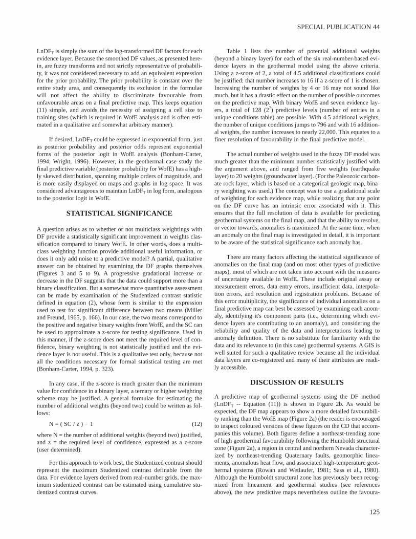
ences are illustrated in Figure 11, which is a map created by subtrac-tion of the WofE grid from the DF grid. These differences are appar-ent along the Humboldt lineament (Figure 2a), where higher inter-mediate rankings of the density function serve to outline the linea-ment better and enhance vectoring toward favourable regions (thisis seen best on the colour version of Figure 11). Another distinctivefeature of the difference map, when viewed in detail (Figure 12), isthe presence of multiple rings or bulls-eyes surrounding areas ofhigh and low favourability. This ringing is a natural result of thefiner subdivisions of favourability ranking in the DF map relative tothe binary WofE map.

CONCLUSIONS

Similarities between the DF and WofE maps should suggest to man-agers and explorationists that WofE is an effective technique in itsown right. Binary WofE predicts geothermal systems well in spiteof converting evidence layers into yes/no, favourable/unfavourableimages (although the binary nature of the WofE maps may havebeen more evident if fewer than seven evidence maps were used).The WofE method also has the advantages of mathematical rigourand providing measures of uncertainty. However, similarities in thetwo maps also help support and justify the DF approach, whichmimics the statistically rigorous WofE method well even though

126


Figure 10. Cumulative area-classification curves compare the prediction of binary weights of evidence to the density function, based on theability to classify training points and geothermal power plants. Curves displaced furthest to the right on the graph indicate better predictivecharacteristics, because fewer geothermal systems would be found in portions of the state with lower favourability rankings. Binary weightsof evidence and the density function appear to predict equally well, based on their classification of 59 training sites and a subset of 10 geot-hermal systems producing electrical energy. However, for both methods, power-producing geothermal systems are predicted better than arethe set of geothermal training points. This suggests that not all training points are created equal, and that power-producing geothermal sys-tems (generally the highest temperature systems) are more dependent on the conjunction of favourable geologic conditions.


127

Figure 11. Difference between the density function (LnDFT) and weights-of-evidence (posterior logit) favourability maps. The two compo-nent maps were rescaled to equal ranges prior to subtraction. Red colours indicate where density function values are higher, blue coloursindicate where weights-of-evidence values are higher. Greater differences tend to occur in the intermediate value ranges. Topographic shad-ing is present in the background.

128


"fuzzy interpolation" is used to interpret smoothed gradational den-sity functions. The advantage of the density method is threefold: itis simple, relatively unbiased, and provides a high density of infor-mation for each evidence layer. It provides a practical alternative inpredictive modelling by stepping carefully outside a purely proba-bilistic framework. In addition, DF modelling can be done with twosimple ratios in a spreadsheet. Such simplicity is of paramountimportance in many work environments.

The multiclass weighting scheme of DF utilizes the entire datadistribution (divided into multiple classes) for each evidence layer;this in turn gives confidence to data experts that the modellingmethod takes full advantage of the available information. Theweighting methods employed are simple and understandable, whichcan make it easier for managers and groups to trust and rely onmodel predictions and reach a consensus on how to act on theresults. The more detailed favourability rankings afforded by the

Figure 12. Difference between the density function and weights-of-evidence maps in west-central Nevada. A pronounced ringing or bulls-eye effect surrounds individual areas of higher favourability (Figures 2a, 2b) and is caused by the finer subdivision of favourability rank-ings in the density function relative to binary weights of evidence. Topographic shading is present in the background.


129

DF method can make it easier to "vector in" and identify anomaliesof potential interest. Not every anomaly may be statistically signif-icant, but a GIS-based review of the causative sources of eachanomaly, conducted quickly and efficiently using the cross-refer-enced and co-located data available on computer, can help deter-mine which anomalies are worthy of follow-up examination.

The mathematics used to calculate densities and combine evi-dence layers remove much of the potential "expert" bias that char-acterizes fuzzy logic methods. Density function weights are similarto weights calculated from WofE; in fact, when training site areasare small relative to the areas of evidence patterns and the totalstudy area, as is often the case in mineral exploration programs, thedensity function calculation represents a simplification of the WofEformulae. Similar to WofE, when some areas of an evidence map donot contain information, a neutral weighting value can be assigned.

The density method described herein differs from multiclassWofE because the raw density values calculated for individual his-togram bins are smoothed by drawing lines or curves linking adja-cent densities on graphs. This is considered necessary because thesubdivision of an evidence layer into multiple histogram bins (mul-tiple patterns) increases the error or uncertainty associated with thedensity calculation, especially when the number of training sites perbin drops to a low number. A similar difficulty affects the accuracyof weight calculations for multiclass WofE. Smoothed density val-ues offer a method of minimizing these errors for real-number basedgrids (ratio data), by relying on information from adjacent his-togram bins. In this study, we have used "expert guidance" to fitcurves to multiclass data, but other more statistically based methodscould be developed and employed, such as linear regression.

ACKNOWLEDGMENTS

This manuscript has benefited from numerous insightful sugges-tions and comments from Gary Raines of the USGS. Jim Taranik,as director of the Great Basin Center for Geothermal Energy, pro-vided key support and encouragement necessary to pursue thisstudy. Mark Mihalasky (USGS) supplied the initial geothermal GISand databases along with his enthusiastic approval for expandingthe scope of work, and Lisa Shevenell of the Nevada Bureau ofMines and Geology made important contributions of geothermaldatabases and interpretations of geothermometer calculations. DonSawatzky (Great Basin Center for Geothermal Energy) providedadvice on structural databases and developed LinAnl, an ArcViewextension for statistical analysis of fault strikes used in this study.Suggestions and comments from several anonymous reviewers andJeff Harris significantly improved the flow, presentation, and rigourof the text, for which we are grateful.

REFERENCES

Agterberg, F.P., 1989, Systematic approach to dealing with uncer-tainty of geoscience information in mineral exploration, inWeiss, A., ed., Applications of Computers and OperationsResearch in the Mineral Industry: Proceedings 21st APCOMSymposium, Las Vegas, Nevada, 27 Feb. - 2 March 1989, p.165-178.

Amor, S., Bloom, L., and Ward, P., 1998, Practical Application ofExploration Geochemistry: Short Course Proceedings, Pros-

pectors and Developers Association of Canada, Toronto,Ontario, 7 March 1998.

Ballantyne, J.M., and Moore, J.N., 1988, Arsenic geochemistry ingeothermal systems: Geochimica et Cosmochimica Acta, v. 52,no. 2, p. 475-483.

Bedell, R.L., 2000, GIS for the Geosciences: Short course volume,National Geological Society of America meeting, Reno,Nevada, Nov. 2000.

Bennett, R.A., Wernicke, B.P., and Davis, J.L., 1998, ContinuousGPS measurements of contemporary deformation across thenorthern Basin and Range Province: Geophysical ResearchLetters, v. 25, no. 4, p. 563-566.

Blackwell, D.D., 1983, Heat flow in the northern Basin and Rangeprovince: Geothermal Resources Council, Special Report No.13, p. 81-92.

Blewitt, G., Coolbaugh, M.F., Holt, W., Kreemer, C., Davis, J.L.,and Bennett, R.A., 2002, Targeting of potential geothermalresources in the Great Basin from regional relationshipsbetween geodetic strain and geological structures: GeothermalResources Council, Transactions, v. 26, p. 523-525.

Bonham-Carter, G.F., 1994, Geographic Information Systems forGeoscientists, Modeling with GIS. Elsevier Science Inc.,Tarrytown, NY, 398 p.

Bonham-Carter, G.F., Agterberg, F.P., and Wright, D.F., 1988,Integration of geological datasets for gold exploration in NovaScotia: Photogrammetric Engineering and Remote Sensing, v.54, no. 11, p. 1585-1592.

Bowen, R., 1989, Geothermal Resources, 2nd Edition: ElsevierScience Inc., New York, NY, 485 p.

Cheng, Q., and Agterberg, F.P., 1999, Fuzzy weights of evidencemethod and its application in mineral potential mapping:Natural Resources Research, v. 8, no. 1, p. 27-35.

Coolbaugh, M.F., Taranik, J.V., Raines, G.L., Shevenell, L.A.,Sawatzky, D.L., Minor, T.B., and Bedell, R.L., 2002, A geo-thermal GIS for Nevada: defining regional controls andfavourable exploration terrains for extensional geothermal sys-tems: Geothermal Resources Council, Transactions, v. 26, p.485-490.

Dohrenwend, J.C., Schell, B.A., Menges, C.M., Moring, B.C., andMcKittrick, M.A., 1996, Reconnaissance photogeologic mapof young (Quaternary and Late Tertiary) faults in Nevada, inSinger, D.A., ed., An Analysis of Nevada's Metal-BearingMineral Resources: Nevada Bureau Mines and Geology,Open-File Report 96-2, p. 9-1 to 9-12.

Drury, S.A., 1993, Image Interpretation in Geology: Chapman andHall, London, UK, 283 p.

Ellis, A.J., and Mahon, W.A.J., 1977, Chemistry and GeothermalSystems: Academic Press, New York, NY, 392 p.

Garside, L., 1994, Nevada low-temperature geothermal resourceassessment: 1994: Nevada Bureau of Mines and Geology,Open File Report 94-2.

Harrill, J.R., and Prudic, D.E., 1998, Aquifer systems in the GreatBasin region of Nevada, Utah, and adjacent states - summaryreport: United States Geological Survey, Professional Paper1409-A, 67 p.

Kemp, L.D., Bonham-Carter, G.F., Raines, G.L., and Looney, C.G.,2001, Arc-SDM: ArcView extension for spatial data modellingusing weights of evidence, logistic regression, fuzzy logic andneural network analysis: http://ntserv.gis.nrcan.gc.ca/sdm/.

Knox-Robinson, C.M., 2000, Vectorial fuzzy logic: a novel tech-nique for enhanced mineral prospectivity mapping, with refer-

130


ence to the orogenic gold mineralisation potential of theKalgoorlie Terrane, Western Australia: Australian Journal ofEarth Sciences, v. 47, p. 929-941.

Koenig, J.B., and McNitt, J.R., 1983, Controls on the location andintensity of magmatic and non-magmatic geothermal systemsin the Basin and Range province: Geothermal ResourcesCouncil, Special Report No. 13, p. 93.

Ludington, S., McKee, E.H., Cox, D.P., Moring, B.C., and Leonard,K.R., 1996, Pre-Tertiary geology of Nevada, in Singer, D.A.,ed., An Analysis of Nevada's Metal-Bearing MineralResources: Nevada Bureau Mines and Geology, Open-FileReport 96-2, p. 9-1 to 9-12.

Mariner, R.H., Presser, T.S., and Evans, W.C., 1982, Geochemistryof active geothermal systems in the northern Basin and Rangeprovince: Geothermal Resources Council, Special Report No.13, p. 95-119.

Mihalasky, M.J., 2006, Controls over the regional-scale distributionof sedimentary and volcanic rock-hosted Au-Ag mineral sitesin Nevada: A GIS-based weights of evidence analysis, inHarris, J.R., ed., GIS for the Earth Sciences: GeologicalAssociation of Canada, Special Publication 44, p. 53-97.

Miller, I., and Freund, J.E., 1965, Probability and Statistics forEngineers: Prentice-Hall Inc., Englewood Cliffs, NJ, 432 p.

Raines, G.L., and Bonham-Carter, G.F., 2006, Exploratory spatialmodelling; demonstration for Carlin-type deposits, centralNevada, USA, using Arc-SDM, in Harris, J.R., ed., GIS for theEarth Sciences: Geological Association of Canada, SpecialPublication 44, p. 23-52.

Raines, G.L., Bonham-Carter, G.F., and Kemp, L., 2000, Predictiveprobabilistic modelling using ArcView GIS: ArcUser, v. 3, no.2, p. 45-48.

Raines, G.L., Sawatzky, D.L., and Connors, K.A., 1996, GreatBasin Geoscience Data Base: United States Geological Survey,Digital Data Series DDS-041.

Pan, G., and Harris, D.P., 2000, Information Synthesis for MineralExploration: Oxford University Press Inc., New York, NY, 461 p.

Richards, M., and Blackwell, D., 2002, The forgotten ones; geother-mal roads less traveled in Nevada: Geothermal ResourcesCouncil, Bulletin, v. 31, no. 2, p. 69-75.

Rowan, L.C., and Wetlaufer, P.H., 1981, Relation between regionallineament systems and structural zones in Nevada: AmericanAssociation of Petroleum Geologists, Bulletin, v. 65, no. 8, p.1414-1432.

Sass, J.H., Blackwell, D.D., Chapman, D.S., Costain, J.K., Decker,E.R., Lawver, L.A., and Swanberg, C.A., 1980, Heat flowfrom the crust of the United States, in Touloukian, Y.S., andHo, C.Y., eds., Physical Properties of Rocks and Minerals:Cindas Data Series on Material Properties: McGraw-Hill, NewYork, NY, p. 13-503 to 13-548.

Sass, J.H., Lachenbruch, A.H., Munroe, R.J., Greene, G.W., andMoses, T.H. Jr., 1971, Heat flow in the Western United States:Journal of Geophysical Research, v. 76, p. 6376-6413.

Shevenell, L., Garside, L.J., and Hess, R.H., 2000, NevadaGeothermal Resources: Nevada Bureau of Mines and Geology,Map 126.

White, D.E., Thompson, J.M., and Fournier, R.O., 1976, Lithiumcontents of thermal and mineral waters, in Vine, J.D., ed.,Lithium Resources and Requirements by the Year 2000:United States Geological Survey, Professional Paper 1005, p.58-60.

Wisian, K.W., Blackwell, D.D., and Richards, M., 1999, Heat flowin the western United States and extensional geothermal sys-tems: Proceedings 24th Workshop on Geothermal ReservoirEngineering, Stanford, CA, p. 219-226.

Wright, D.F., 1996, Evaluating volcanic hosted massive sulfidefavourability using GIS-based spatial data integration models,Snow Lake area, Manitoba: Ph.D. thesis, University ofOttawa, Ottawa, ON, 344 p.

Documents

Chapter 5 A Simplification of Weights of Evidence using a ... · A Simplification of Weights of Evidence using a Density Function and Fuzzy Distributions; Geothermal Systems, Nevada